Pépite | Vers un critère de dommage en fatigue d'acier pour pipelines basé sur des changements microstructuraux
177
0
0
Texte intégral
(2) Thèse de Geovana Pereira Drumond, Université de Lille, 2019. ACKNOWLEDGMENTS : Firstly, I would like to express my sincere gratitude to my advisors Prof. Ilson Paranhos Pasqualino, Prof. Francine Roudet and Prof. Bianca de Carvalho Pinheiro for the continuous support during my Ph.D studies, for their patience, motivation, inspiration, and valuable expertise. I am extremely thankful to Prof. Didier Chicot for the guidance during the different phases of the work, from the understanding of the subject to the interpretation of results. I would like to thank Prof. Marcelo Igor Lourenço de Souza, from the Federal University of Rio de Janeiro, Prof. Jean-Loius Robert, from the Université Clermont Auvergne, Prof. José Luiz de França Freire, from the Pontifical Catholic University of Rio de Janeiro, and Prof. Marie-José Pac, from the Université de Haute-Alsace, members of the jury, for their valuable contribution with insightful comments. I would like to thank their time and dedication spent reading and examining the thesis. I am really grateful to the whole administration and technical staff of the Subsea Technology Laboratory (LTS) of COPPE/Federal University of Rio de Janeiro, and of the IUT A – GMP of the University of Lille for all support spent in different moments during the accomplishment of this work. I would also like to express my gratitude to my friends from the IUT A – GMP, Dr. Xavier Decoopman, Dr. Cosmin Gruescu, Dr. Stephania Kossman, Dr. Philémon Nogning, Dr. Alberto Mejias, Dr. Mohammed Bouchelarm for sharing his friendship, helping me in several tasks, and sharing valuable insights and motivating conversations. My sincere thanks also go to Laurence Lagaisse, secretary of the IUT A – GMP, for always helping me with administrative questions. I would like to show my gratitude to everyone who helped me in different ways to offer me a wonderful and unforgettable time in France. I am extremely thankful to the financial support from Capes-Cofecub program number 800-14, essential for the accomplishment of this work. Finally, I would like to thank all my friends and family, and in special my parents, Sérgio Luis Drumond and Maria das Graças Soares Pereira Drumond, my grandmother Coracira Soares Pereira, and in memory, my grandfather Manoel Rocha Pereira, for supporting me throughout my life. ii © 2019 Tous droits réservés.. lilliad.univ-lille.fr.
(3) Thèse de Geovana Pereira Drumond, Université de Lille, 2019. TITRE EN FRANÇAIS : VERS UN CRITERE DE DOMMAGE EN FATIGUE D'ACIER POUR PIPELINES BASE SUR DES CHANGEMENTS MICROSTRUCTURAUX. RESUMÉ : L’étude des modifications de la microdureté de la surface des matériaux au cours des différentes étapes de la fatigue peut permettre d’évaluer l’évolution de la résistance des matériaux aux déformations microplastiques et ainsi fournir des informations pertinentes sur les dommages cumulés causés par la fatigue à la surface. L’objectif de ce travail est de proposer une nouvelle méthode basée sur les changements microstructuraux pour prédire la durée de vie en fatigue des structures en acier soumises à des charges cycliques, avant la fissuration macroscopique. Des essais d’indentation instrumentée et des analyses par diffraction des rayons X ont été effectués sur des échantillons soumis à grand nombre de cycles (de l’anglais, High Cycle Fatigue -HCF), jusqu’à différentes fractions de sa durée de vie en fatigue. Il a été observé que les changements majeurs dans les valeurs de microdureté se produisaient à la surface du matériau, jusqu’à 2 µm de profondeur d’indentation, et à environ 20% de la durée de vie en fatigue des échantillons, ce qui était attendu, car les étapes de nucléation et de microfissuration des fissures sont des phénomènes de surface. Ici, la valeur de 20% de la durée de vie en fatigue a été déterminée comme la période critique pour les changements microstructuraux, et cette valeur a été utilisée dans un ajustement analytique d'une expression polynomiale afin de prédire le nombre de cycles em fatigue jusqu’à rupture (Nf) d'une structure en acier.. MOTS-CLÉS : Amorçage. de. l’endommagement. par. Fatigue;. Microdéformations;. Essais. de. Microindentation Instrumentés; Diffraction des rayons X; Acier API 5L X65; Pipelines. iii © 2019 Tous droits réservés.. lilliad.univ-lille.fr.
(4) Thèse de Geovana Pereira Drumond, Université de Lille, 2019. TÍTULO EM POTUGUÊS : PROPOSTA DE CRITÉRIO DE AVALIAÇÃO DE DANOS EM FADIGA DE OLEODUTOS DE AÇO COM BASE EM MUDANÇAS MICROESTRUTURAIS. RESUMO : O estudo das variações dos valores de microdureza na superfície durante a vida em fadiga do material pode ser usado para estimar a evolução da resistência do material às deformações microplásticas e, consequentemente, fornecer informações relevantes sobre os danos acumulados na superfície. O objetivo deste trabalho é propor uma nova metodologia baseada em mudanças microestruturais para prever a vida em fadiga de estruturas de aço submetidas à carga cíclicas antes da propagação macroscópica de trincas. Testes de microindentação instrumentada e análises de difração de raios-X foram realizados nas amostras, previamente submetidas a ensaios de fadiga de alto ciclo, em diferentes frações da vida em fadiga do material. Observou-se que as grandes mudanças nos valores de microdureza ocorreram na superfície e subsuperfície do material, até 2μm de profundidade de penetração, e a cerca de 20% da vida de fadiga das amostras, o que era esperado, uma vez que a nucleação e propagação de microtrincas são fenômenos que ocorrem preferencialmente na superfície do material. No presente trabalho, o valor de 20% da vida em fadiga foi determinado como o período crítico para mudanças microestruturais, e esse valor foi usado em um ajuste analítico através de uma expressão polinomial para prever o número de ciclos até a falha (Nf) de uma estrutura de aço.. PALAVRAS-CHAVE : Dano por fadiga; Microdeformações; Testes de microindentação instrumentada; Difração de Raios-X; Aço API 5L X65; Dutos de transporte de petróleo (pipelines). iv © 2019 Tous droits réservés.. lilliad.univ-lille.fr.
(5) Thèse de Geovana Pereira Drumond, Université de Lille, 2019. TITLE IN ENGLISH : TOWARDS A PROPOSAL OF FATIGUE DAMAGE ASSESSMENT OF STEEL PIPELINES BASED ON MICROSTRUCTURAL CHANGES. ABSTRACT : The study of changes in material surface microhardness during the different stages of the fatigue mechanisms can be used to estimate the evolution of the material resistance to microplastic deformations and, consequently, provide relevant information about the cumulated fatigue damage on the surface. The aim of this work is to propose a new methodology based on microstructural changes to predict fatigue life of steel structures submitted to cyclic loading, before macroscopic cracking. Instrumented indentation tests and X-Ray diffraction analysis were carried out in the samples previously submitted to high cycle fatigue (HCF) loads, up to different fatigue life fractions. It was observed that the major changes in the microhardness values occurred at the surface and subsurface of the material, up to 2 µm of indentation depth below the surface, and around 20% of the fatigue life of the steel samples, which was expected, since crack nucleation and microcracking stages result of surface phenomena. Here, the value of 20% of the fatigue life was determined as the critical period for microstructural changes, and this value was used in an analytical fit of a polynomial expression to predict the number of cycles to failure (Nf) of a steel structure.. KEYWORDS : Fatigue damage; Microstructural changes; Instrumented microindentation tests; XRay Diffraction; API 5L X65 steel; Pipelines. v © 2019 Tous droits réservés.. lilliad.univ-lille.fr.
(6) Thèse de Geovana Pereira Drumond, Université de Lille, 2019. TABLE OF CONTENTS LIST OF FIGURES .................................................................................................................... viii LIST OF TABLES .................................................................................................................... xvii INTRODUCTION ........................................................................................................................2 STRUCTURE OF THE DISSERTATION ...........................................................................................4 CHAPTER I. FATIGUE OF METALS .......................................................................................7 I.1 STRESS-LIFE METHOD .......................................................................................................8 I.2 FATIGUE DAMAGE IN HIGH CYCLE FATIGUE .................................................................15 I.2.1 MICROCRACK NUCLEATION ............................................................................................17 I.2.2 MICROCRACK PROPAGATION ..........................................................................................18 CHAPTER II. INDENTATION HARDNESS .............................................................................21 II.1 MICROINDENTATION HARDNESS TESTING ....................................................................21 II.2 MICROHARDNESS TESTING APPLIED TO FATIGUE DAMAGE ASSESSMENT ..................29 CHAPTER III. X-RAY DIFFRACTION ..................................................................................42 III.1 PRINCIPLES OF X-RAY DIFFRACTION ...........................................................................42 III.2 METHODS OF PEAK BROADENING ANALYSIS ...............................................................46 III.3 X-RAY. DIFFRACTION. APPLIED. TO. MECHANICAL CHARACTERIZATION. OF. MATERIALS ............................................................................................................................48 CHAPTER IV. MATERIAL CHARACTERIZATION ................................................................64 IV.1 UNIAXIAL TENSION TESTS.............................................................................................64 IV.2 CHEMICAL COMPOSITION ANALYSES ...........................................................................67 IV.3 METALLOGRAPHIC ANALYSES ......................................................................................68 CHAPTER V. EXPERIMENTAL TESTS .................................................................................76 V. 1 FATIGUE TESTS...............................................................................................................76 V.1.1 EXPERIMENTAL SETUP ...................................................................................................76 V.1.2 CALIBRATION OF THE FATIGUE MACHINE......................................................................77 vi © 2019 Tous droits réservés.. lilliad.univ-lille.fr.
(7) Thèse de Geovana Pereira Drumond, Université de Lille, 2019. V.1.3 FATIGUE TEST SAMPLES ................................................................................................78 V1.4 S-N CURVE .....................................................................................................................80 V.2 INDENTATION TESTS .......................................................................................................81 V.3 X-RAY DIFFRACTION TESTS ...........................................................................................88 CHAPTER VI. RESULTS AND DISCUSSION ..........................................................................92 VI.1 INSTRUMENTED INDENTATION RESULTS ......................................................................94 VI. 2 X-RAY DIFFRACTION RESULTS ..................................................................................119 VI.3 COMPARISON OF THE INDENTATION AND X-RAY RESULTS .......................................136 CONCLUSIONS AND PERSPECTIVES .....................................................................................143 FUTURE WORKS ....................................................................................................................144 REFERENCES ........................................................................................................................149. vii © 2019 Tous droits réservés.. lilliad.univ-lille.fr.
(8) Thèse de Geovana Pereira Drumond, Université de Lille, 2019. LIST OF FIGURES Figure I-1:Typical stress history during cyclic loading [21]. _________________________ 8 Figure I-2: (a) S-N curves for σm ≠ 0; (b) Gerber, Goodman and Soderberg curves [23]. __ 9 Figure I-3: S-N curves in log-log and semi-log scales for superalloy S/SAV [22]. _______ 10 Figure I-4: Ferrous and nonferrous S-N curves [22]. ______________________________ 11 Figure I-5: S-N curve (log-log) scale for steel [22]. _______________________________ 11 Figure I-6: Correlation between the ultimate strength and endurance limit [23]. ________ 12 Figure I-7: S-N curve plotted from results of completely reversed axial fatigue tests. Material: normalized UNS G41300 steel. Adapted from [15]. ______________________ 14 Figure I-8: Value of f as a function of 𝑆𝑢𝑡 [20]. _________________________________ 15 Figure I-9:Schema of stages I and II of fatigue crack growth in an AlZnMg alloy [15]. __ 16 Figure I-10: Atomic rearrangements that accompany the motion of an edge dislocation as it moves in response to an applied shear stress. Adapted from [15]. _____________________ 18 Figure I-11: Damage mechanism of development of a persistent slip band (PSB) and an irreversible step at the surface. Adapted from [15]. ________________________________ 18 Figure I-12: Model for the mechanism of formation of slip band extrusions and intrusions proposed by Wood [78]. (a) Static deformation. (b) Cyclic deformation leading t surface notch (intrusion) and (c) surface ridge (extrusion). Adapted from [15]. ________________ 18 Figure II-1: Comparison of Knoop and Vickers microindentations [35]. ______________ 23 Figure II-2: (a) Elasto-plastic deformation at the maximum applied load Pmax; (b) plastic deformation after releasing the load [35]. ______________________________________ 24 Figure II-3: Schematic load-indenter displacement curve obtained from instrumented indentation test [35]. _______________________________________________________ 24 Figure II-4: (a) Berkovich and (b) Vickers projected areas._________________________ 25 Figure II-5: Representation of piling-up and sinking-in during an instrumented indentation test [46]. ________________________________________________________________ 27 viii © 2019 Tous droits réservés.. lilliad.univ-lille.fr.
(9) Thèse de Geovana Pereira Drumond, Université de Lille, 2019. Figure II-6: The change of microhardness mean of ferrite and pearlite during cycles: (A) ferrite; (B) _______________________________________________________________ 29 Figure II-7: Cycle-dependent changes in tensile curve [50]. ________________________ 30 Figure II-8: Geometric scheme of a pyramidal indenter penetrating into a specimen surface (X1, X2, X3, Cartesian coordinates): P, load; d, imprint diagonal; h, indentation depth; he, elastic backformation; hp plastic deformation [50]. _______________________________ 31 Figure II-9: Diagram of Vickers hardness vs. deformation for several different states of a material [50]. ____________________________________________________________ 32 Figure II-10: Variation of Vickers microhardness with the number of cycles in (a) annealed 16Mn steel, (b) normalized 45# steel [50]. ______________________________________ 32 Figure II-11: Evolution of surface damage in different constitutive phases, ferrite and pearlite, during cycling [49]. ________________________________________________ 35 Figure II-12: Cross-sectional geometry and transversal micrograph of the artificial defect: relationship between applied load and plastic deformation at the tip of the indentation [51]. _______________________________________________________________________ 36 Figure II-13: Influence of the materiaç constants on the fatigue limit for high hardness steels [53] ____________________________________________________________________ 39 Figure II-14: Influence of material constants on the threshold of stress intensity factor for high hardness steels [53]. ___________________________________________________ 39 Figure III-1: A lattice point , where d is the lattice spacing [60]. ____________________ 43 Figure III-2: Schematic of x-ray diffraction; (a) illustration of the conditions required for Bragg diffraction to occur and (b) relationship of the incident (k0), diffracted (kh) and scattering (S) vectors with respect to the crystal [59]. _____________________________ 44 Figure III-3: Schema of XRD measurement and XRD peak, characterized by the angular position 2θ and the full width at half maximum (FWHM). _________________________ 45 Figure III-4: Effects of lattice deformation on XRD peaks for (a) nondeformed material, (b) uniform deformation (macrostresses), and (c) nouniform deformation (microdeformations) [15]. ___________________________________________________________________ 45 Figure III-5: Depth profiles for various fractions of the total fatigue life of A1 2024 ix © 2019 Tous droits réservés.. lilliad.univ-lille.fr.
(10) Thèse de Geovana Pereira Drumond, Université de Lille, 2019. specimens, obtained by incrementally removing surface layers and carrying out X-ray analysis with CuX; radiation at each depth [101]. ________________________________ 49 Figure III-6:Diagram for Al 2024 specimens given prior fatigue cycling to 75 and 95% of their fatigue life at ±200 MPa, followed by surface removal and recycling treatment (A and B), and either continued recycling or a second depth profile analysis (C) [101]. ________ 50 Figure III-7:The half-breadth of 220 peak (FWHM) and longitudinal residual stress and the microstrain in the[110] direction vs. depth for the high cycle fatigue (a) 78340 cycles of normalized AIS11008 steel; and (b) 90000 cycles of cold-worked AISI 1008 steel [103]._ 51 Figure III-8: b/b0 vs N data at (a) 32 MPa and (b) 46 MPa. Dashed line represents the average curve [102]. _______________________________________________________ 52 Figure III-9: A typical, three-stage b/b0 vs N curve when the diffraction patterns are recorded from the near-surface region of the specimen. The three stages are marked as I, II and III respectively [104]. __________________________________________________ 52 Figure III-10: Variation of microstrain E with N [102].____________________________ 53 Figure III-11: Macrostresses and microstresses along the loading direction with fatigue at 276 MPa in (a) peartite, (b) spheroidite, (c) tempered martensite, and (d) shot-peened spheroidite sample [105]. ___________________________________________________ 54 Figure III-12: Individual peak analysis of the XRDCD data for AISI304. Comparison of the combined results from the Δε = 0.60% and Δε = 1.20% regimes (top) and the combined results from near surface and bulk for the A€ = 0.60% regime (bottom). near surface,. Δε= 1.20% near surface,. Δε = 0.60%. Δε= 0.60% bulk. The solid symbols. represent results which have a statistically significant difference from the initial state; and, the outlined symbols represent results which have no statistically significant difference from the initial state [99]. _______________________________________________________ 55 Figure III-13: Individual peak analysis of the XRDCD data for AISI304. Comparison of the combined results from the near surface and subsurface for the both the Δε = 0.60% and Δε = 1.20% regimes at 5% N/Nf (top), 50% N/Nf (middle), and failure (bottom). The solid horizontal bars represent the initial state values from the Δε = 1.20% regime, and the broken horizontal bars represent the initial state values from the Δε = 0.60% regime. 0.60% regime,. Δε =. Δε = 1.20% regime. The solid symbols represent results which have a x. © 2019 Tous droits réservés.. lilliad.univ-lille.fr.
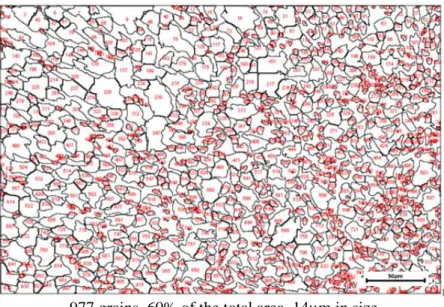
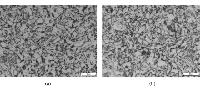
(11) Thèse de Geovana Pereira Drumond, Université de Lille, 2019. statistically significant difference from the initial state; and, the outlined symbols represent results which have no statistically significant difference from the initial state [99]. ______ 56 Figure III-14: Variance analysis of the XRDCD data for SAS08. Comparison of the combined results from the Δε = 0.48% and Δε = 0.78% regimes (top) and the combined results from near surface and bulk for the Δε=0.78% regime (bottom). O Δε = 0.48% near surface,. Δε = 0.78% near surface,. Δε = 0.78% bulk [99]. ______________________ 56. Figure III-15: Characteristic (220) XRD line of AISI 316L stainless steel (Cr Kα radiation): integral breadth β is evaluated on Kα1 component of peak [100].____________________ 58 Figure III-16: Results of β measurements on surface of untreated and laser treated AISI 316L specimens fatigued at load of 500 MPa [100]. ______________________________ 59 Figure III-17: Change of half value breadth with number of cycles: (a) Al phase; (b) SiC phase [97]. ______________________________________________________________ 60 Figure III-18: Change of full width at half maximum with number of stress cycles: (a) aluminum phase; (b) SiC phase [98]. __________________________________________ 61 Figure III-19: Evolution of FWHM and residual stresses σR with fatigue cycling at (a) σa = 277 MPa and R=-1; (b) σa = 361 MPa and R=-1; (c) σa = 319 MPa and R=-1; (d) σa =367 MPa and R=−2.8 [109]. ____________________________________________ 62 Figure IV-1: Test coupons and samples cut off from an API 5L X65 grade steel pipe for:(a) uniaxial tension tests and (b) fatigue, indentation and X-Ray tests.___________________ 64 Figure IV-2: Tensile samples, where w1 = 20 mm, w2 = 30 mm, l = 40 mm, and t = 3 mm. _______________________________________________________________________ 65 Figure IV-3: Stress-Strain curves for API X65 steel as-machined samples. ____________ 65 Figure IV-4: Stress-Strain curves for API X65 steel annealed samples. _______________ 66 Figure IV-5: Microstructure of an as-machined specimen observed through optical microscope, magnification factor of (a) 100x, (b) 200x, (c) 500x and (d) 1000x. ________ 69 Figure IV-6: Microstructure of an annealed specimen observed through optical microscope, magnification factor of (a) 100x, (b) 200x, (c) 500x and (d) 1000x. __________________ 69 Figure IV-8: Image J analyses of grain size for an as-machined sample with 200x of magnification factor. _______________________________________________________ 70 xi © 2019 Tous droits réservés.. lilliad.univ-lille.fr.
(12) Thèse de Geovana Pereira Drumond, Université de Lille, 2019. Figure IV-9: Image J analyses of grain size for an annealed sample with 200x of magnification factor. _______________________________________________________ 70 Figure IV-10: Fatigue cycled specimen with the red square indicating where the metallographic examinations were done. _______________________________________ 71 Figure IV-11: Microstructure of an as-machined specimen observed through optical microscope, magnification factor of 500x, (a) non-cycled and (b) after fatigue failure. ___ 72 Figure IV-12: Microstructure of an annealed specimen observed through optical microscope, magnification factor of 500x, (a) non-cycled and (b) after fatigue failure. _____________ 72 Figure IV-13: Image J grain size analyses of an as-machined sample, magnification factor of 200x, (a) non-cycled and (b) after fatigue failure. ________________________________ 73 Figure IV-14: Image J grain size analyses of an annealed sample, magnification factor of 200x, (a) non-cycled and (b) after fatigue failure. ________________________________ 74 Figure V-1: (a) Schenck fatigue machine; (b) Positioning of the samples at the machine. _ 76 Figure V-2: Schematic representation of the alternating bending fatigue testing machine [119]. __________________________________________________________________ 77 Figure V-3: Geometry and dimensions (in mm) of fatigue test samples. ______________ 78 Figure V-4: (a) Struers Lectropol 5 device, (b) Positioning of the samples at the machine. 79 Figure V-5: Geometry and dimensions of the surface electrolytically polished. _________ 80 Figure V-6: Estimated S-N curves for as-machined and annealed conditions. __________ 81 Figure V-7: Experimental setup for microindentation tests. ________________________ 82 Figure V-8: Microhardness tests samples (dimensions in millimeters). _______________ 82 Figure V-9: Curve load vs penetration depth for 20 cycles of indentation. _____________ 83 Figure V-10: Impressions made with a Berkovich indenter (three-sided pyramid). ______ 83 Figure V-11: Flow chart of the indentation analysis methodology. ___________________ 86 Figure V-12: Excel Macro developed to execute all the steps of the methodology adopted for the microhardness analysis. _________________________________________________ 87 Figure V-13: Screen display of software results. _________________________________ 88 xii © 2019 Tous droits réservés.. lilliad.univ-lille.fr.
(13) Thèse de Geovana Pereira Drumond, Université de Lille, 2019. Figure V-14: Experimental setup for X-ray diffraction measurements with the portable mode of the Proto iXRD diffractometer and the fatigue machine._________________________ 89 Figure V-15: (a) Experimental setup for X-Ray diffraction measurements in the sample longitudinal direction (X-Ray detectors L1 and R2), and (b) schematic representation of the X-Ray diffractometer. Adapted from [15]. ______________________________________ 90 Figure VI-1: Comparison between the estimated (in black) and experimental (in red) Basquin equation for as-machined samples._____________________________________ 93 Figure VI-2: Comparison between the estimated (in black) and experimental (in red) Basquin equation for annealed samples.________________________________________ 93 Figure VI-3: Sample geometry. ______________________________________________ 97 Figure VI-4: Distribution of alternating stress amplitudes in the sample. ______________ 99 Figure VI-5: Variation of hardness during fatigue life for as-machined X-65 steel samples.99 Figure VI-6: Variation of hardness during fatigue life for annealed X-65 steel samples. _ 100 Figure VI-7: Hardness versus depth of penetration curves for the as-machined sample T2EF32, cycled until 7% of the fatigue life. ___________________________________ 102 Figure VI-8: Hardness versus depth of penetration curves for the as-machined sample T2EF34, cycled until 11% of the fatigue life. __________________________________ 103 Figure VI-9: Hardness versus depth of penetration curves for the as-machined sample T2EF21R, cycled until 7% of the fatigue life. __________________________________ 103 Figure VI-10: Hardness versus depth of penetration curves for the as-machined sample T2EF22R, cycled until 19% of the fatigue life. _________________________________ 104 Figure VI-11: Variation of hardness during fatigue life for all stress amplitudes studied at a penetration depth of 2µm from surface for as-machined samples. __________________ 105 Figure VI-12: Variation of hardness during fatigue life for all stress amplitudes studied at a penetration depth of 4µm from surface for as-machined samples. __________________ 105 Figure VI-13: Variation of hardness during fatigue life for all stress amplitudes studied at a penetration depth of 6µm from surface for as-machined samples. __________________ 106 Figure VI-14: Variation of hardness during fatigue life for all stress amplitudes studied at a xiii © 2019 Tous droits réservés.. lilliad.univ-lille.fr.
(14) Thèse de Geovana Pereira Drumond, Université de Lille, 2019. penetration depth of 2µm from surface for annealed samples. _____________________ 106 Figure VI-15: Variation of hardness during fatigue life for all stress amplitudes studied at a penetration depth of 4µm from surface for annealed samples. _____________________ 107 Figure VI-16: Variation of hardness during fatigue life for all stress amplitudes studied at a penetration depth of 6µm from surface for annealed samples. _____________________ 107 Figure VI-17: Microhardness changes during fatigue life at 2µm for σ = 171 MPa._____ 109 Figure VI-18: Microhardness changes during fatigue life at 2µm for σ = 225 MPa._____ 109 Figure VI-19:Microhardness changes during fatigue life at 2µm for σ = 255 MPa. _____ 110 Figure VI-20: Microhardness changes during fatigue life at 2µm for σ = 272 MPa._____ 110 Figure VI-21: Microhardness changes during fatigue life at 2µm for σ = 335 MPa._____ 111 Figure VI-22: Microhardness changes during fatigue life at 2µm for σ = 358 MPa._____ 111 Figure VI-23: Microhardness changes during fatigue life at 2µm for σ = 171 MPa._____ 113 Figure VI-24: Microhardness changes during fatigue life at 2µm for σ = 225 MPa._____ 113 Figure VI-25: Microhardness changes during fatigue life at 2µm for σ = 255 MPa._____ 114 Figure VI-26: Microhardness changes during fatigue life at 2µm for σ = 272 MPa._____ 114 Figure VI-27: Microhardness changes during fatigue life at 2µm for σ = 335 MPa._____ 115 Figure VI-28: Microhardness changes during fatigue life at 2µm for σ = 358 MPa._____ 115 Figure VI-29: Graphic comparison between the values of experimental Nf and the values obtained by adjustment of polynomials for as-machined samples. __________________ 118 Figure VI-30: Graphic comparison between the values of experimental Nf and the values obtained by adjustment of polynomials for annealed samples. _____________________ 118 Figure VI-31: Crack propagation during cycling. _______________________________ 119 Figure VI-32: Evolution of FWHM with fatigue cycling at σa= 272 MPa (R=-1) for the sample T2EF55. _________________________________________________________ 121 Figure VI-33: Evolution of FWHM with fatigue cycling at σa= 272 MPa (R=-1) for the sample T2EF61. _________________________________________________________ 121 xiv © 2019 Tous droits réservés.. lilliad.univ-lille.fr.
(15) Thèse de Geovana Pereira Drumond, Université de Lille, 2019. Figure VI-34: Evolution of FWHM with fatigue cycling at σa= 358 MPa (R=-1) for the sample T2EF45. _________________________________________________________ 122 Figure VI-35: Evolution of FWHM with fatigue cycling at σa= 358 MPa (R=-1) for the sample T2EF53. _________________________________________________________ 122 Figure VI-36: Evolution of FWHM with fatigue cycling at σa= 358 MPa (R=-1) for the sample T2EF59. _________________________________________________________ 123 Figure VI-37: Evolution of FWHM with fatigue cycling at σa= 358 MPa (R=-1) for the sample T2EF60. _________________________________________________________ 123 Figure VI-38: Evolution of FWHM with fatigue cycling at σa= 358 MPa (R=-1) for the sample T2EF62. _________________________________________________________ 124 Figure VI-39: Evolution of FWHM with fatigue cycling at σa= 358 MPa (R=-1) for the sample T2EF63. _________________________________________________________ 124 Figure VI-40: Evolution of FWHM vs number of cycles at σa= 272 MPa (R=-1) for the sample T2EF55. _________________________________________________________ 126 Figure VI-41: Evolution of FWHM vs number of cycles at σa= 272 MPa (R=-1) for the sample T2EF61. _________________________________________________________ 126 Figure VI-42: Evolution of FWHM vs number of cycles at σa= 358 MPa (R=-1) for the sample T2EF45. _________________________________________________________ 127 Figure VI-43: Evolution of FWHM vs number of cycles at σa= 358 MPa (R=-1) for the sample T2EF53. _________________________________________________________ 127 Figure VI-44: Evolution of FWHM vs number of cycles at σa= 358 MPa (R=-1) for the sample T2EF59. _________________________________________________________ 128 Figure VI-45: Evolution of FWHM vs number of cycles at σa= 358 MPa (R=-1) for the sample T2EF60. _________________________________________________________ 128 Figure VI-46: Evolution of FWHM vs number of cycles at σa= 358 MPa (R=-1) for the sample T2EF62. _________________________________________________________ 129 Figure VI-47: Evolution of FWHM vs number of cycles at σa= 358 MPa (R=-1) for the sample T2EF63. _________________________________________________________ 129 xv © 2019 Tous droits réservés.. lilliad.univ-lille.fr.
(16) Thèse de Geovana Pereira Drumond, Université de Lille, 2019. Figure VI-48: Graphic comparison between the values of experimental Nf and the values obtained by the method of adjustment of polynomials. ___________________________ 131 Figure VI-49: Evolution of FWHM vs Nf at σa= 358 MPa (R=-1) for the annealed sample T2EF48R. ______________________________________________________________ 132 Figure VI-50: Evolution of FWHM vs Nf at σa= 358 MPa (R=-1) for the annealed sample T2EF56R. ______________________________________________________________ 132 Figure VI-51: Evolution of FWHM vs Nf at σa= 358 MPa (R=-1) for the annealed sample T2EF57R. ______________________________________________________________ 133 Figure VI-52: Evolution of FWHM vs Nf at σa= 358 MPa (R=-1) for the annealed sample T2EF58R. ______________________________________________________________ 133 Figure VI-53: Microstructure of an annealed specimen observed through optical microscope, magnification factor of (a) 100x, (b) 200x, (c) 500x and (d) 1000x. _________________ 134 Figure VI-54: Comparison between the microstructure of samples treated in (a) Brazil and (b) France. ______________________________________________________________ 135 Figure VI-55: Comparison between (a) indentation and (b) X-Ray results for a stress amplitude of 272 MPa. ____________________________________________________ 137 Figure VI-56: Comparison between (a) indentation and (b) X-Ray results for a stress amplitude of 358 MPa. ____________________________________________________ 138 Figure VI-57: Graphic comparison between the values of predicted Nf for X-ray and indentation analysis. ______________________________________________________ 139 Figure VI-58: Load versus penetration depth curve for 20 cycles of indentation for a instrumented indentation test with zoom in the area with hi<2μm, where dynamic indentation analysis could be done. __________________________________________ 146. xvi © 2019 Tous droits réservés.. lilliad.univ-lille.fr.
(17) Thèse de Geovana Pereira Drumond, Université de Lille, 2019. LIST OF TABLES Table IV-1: Average mechanical properties obtained for API 5L X65 grade steel asmachined and annealed samples. _____________________________________________ 66 Table IV-2: Minimum and maximum tensile requirements for API 5L X65 grade steel [113] _______________________________________________________________________ 66 Table IV-3: Average chemical composition in percentage of weight (wt. %) estimated for API 5L X65 grade steel. ____________________________________________________ 68 Table IV-4: Maximum chemical composition requirements in percentage of weight (. %) for API 5L X65 grade steel by the standard API SPEC 5L. ___________________________ 68 Table V-1: Calibration of the fatigue testing machine. ____________________________ 78 Table V-2: Parameters of XRD measurements. __________________________________ 88 Table VI-1: Samples tested for a stress amplitude of 272 MPa. _____________________ 95 Table VI-2: Samples tested for a stress amplitude of 358 MPa. _____________________ 95 Table VI-3: Fatigue cycled samples under 272 and 358 MPa of applied stress amplitudes, values in percentage._______________________________________________________ 96 Table VI-4: Comparison of initial hardness values for as-machined and annealed samples. ______________________________________________________________________ 101 Table VI-5: Minimum/maximum x value measured at 2000 nm as a function of the stress amplitude between 171 and 358 MPa. ________________________________________ 112 Table VI-6: Minimum/maximum x value measured at 2µm as a function of the stress amplitude between 171 and 358 MPa. ________________________________________ 116 Table VI-7: Comparison between the values of experimental Nf and the values obtained by the method of adjustment of polynomials for as-machined samples._________________ 117 Table VI-8: Comparison between the values of experimental Nf and the values obtained by the method of adjustment of polynomials for annealed samples.____________________ 117 Table VI-9: Samples submitted to X-Ray diffraction analysis. _____________________ 120 Table VI-10: : Inflection points obtained for the X-Ray samples. ___________________ 125 xvii © 2019 Tous droits réservés.. lilliad.univ-lille.fr.
(18) Thèse de Geovana Pereira Drumond, Université de Lille, 2019. Table VI-11: Inflection points obtained for the X-Ray samples (number of cycles). ____ 130 Table VI-12: Comparison between the values of experimental Nf and the values obtained by the method of adjustment of polynomials. _____________________________________ 130. xviii © 2019 Tous droits réservés.. lilliad.univ-lille.fr.
(19) Thèse de Geovana Pereira Drumond, Université de Lille, 2019. INTRODUCTION. © 2019 Tous droits réservés.. lilliad.univ-lille.fr.
(20) Thèse de Geovana Pereira Drumond, Université de Lille, 2019. TOWARDS A PROPOSAL OF FATIGUE DAMAGE ASSESSMENT OF STEEL PIPELINES BASED ON MICROSTRUCTURAL CHANGES. INTRODUCTION The world energy matrix is still dependent of the hydrocarbons fuels provided by the oil and gas industry. These inputs are of difficult substitution in the world energy matrix and are the basis of the production and consumption mode and even the culture of modern society [1]. A way to demonstrate the economic strength of the oil industry is to understand the economic importance of the oil companies in a world context. Among the 25 largest companies in the world, 6 (Shell, Exxon Mobil, Chevron, PetroChina, BP and Total) are from the oil and gas sector; among the top 100, 11 are in the oil industry (the six above, plus GazProm, Petrobras, Equinor, Eni and Luk Oil) [2]. Oil and gas exploration and production in deepwater is associated with the use of highly sophisticated equipment and increasing innovative technology. However, the failure of this equipment can cause serious consequences, including material loss and environmental pollution. Critical accidents can even cause the loss of human lives [3]. Pipelines are the safest method to export liquid and gaseous petroleum products or chemicals.. However, like any engineering structure, pipelines do occasionally fail.. According to Drumond et al. [3], the main failure modes experienced by pipelines during production are identified as mechanical damage (impact or accidental damage), external and/or internal corrosion, construction defect, material or mechanical failure, natural hazards and fatigue. The phenomenon of metal fatigue presents a complex nature, involving several stages. These stages can be successively identified as microcrack initiation and propagation (Stage I), macrocrack propagation (Stage II) and final fracture (Stage III). Fatigue crack growth rates in Stages I and II have been extensively studied for decades in materials of different microstructures, evidencing some common features of the crack propagation behavior [4]. Stage I crack growth occurs along crystallographic slip bands and is dominated by shear. Stage II crack growth is associated with crack propagation on a plane normal to the direction of the maximum principal tensile stress applied, involving simultaneous or alternating plastic flow along two slip systems forming striations on the fracture surface [4-8]. Several numerical simulation models were developed to predict the fatigue crack growth in materials based on the relation of the crack growth rate and fatigue loading parameters, such as the linear elastic fracture mechanics (LEFM) approach based on the 2 © 2019 Tous droits réservés.. lilliad.univ-lille.fr.
(21) Thèse de Geovana Pereira Drumond, Université de Lille, 2019. TOWARDS A PROPOSAL OF FATIGUE DAMAGE ASSESSMENT OF STEEL PIPELINES BASED ON MICROSTRUCTURAL CHANGES. Paris law [9]. However, this approach is more suitably applied for modeling the fatigue crack propagation in Stage II, when the crack growth is regular and stable. However, in Stage I, modeling of the fatigue crack growth behavior needs a deeper understanding of the microstructural mechanisms [4]. Some assumptions were made trying to better understand the microstructural mechanisms involved in the Stage I fatigue crack growth, in which the microstructural features, such as grain boundaries, grain size and grain orientation, as well as the sample geometry, influence the fatigue microcrack growth [4]. Bjerkén and Melin [10,11] show that the growth of the fatigue microcracks is driven by shear and is dominated by local plasticity, and these micromechanisms are accompanied by the formation of a local plastic zone ahead of the crack tip, while Andersson and Persson [12] and Jono et al. [13] show that the crack growth occurs along preferred slip planes. According to Ye and Wang [14], a great deal of experimental evidence has proved that fatigue damage in the first stage is primarily related to the occurrence and development of localized plastic strain concentration at or near the surface of materials during cycling. The investigation of the fatigue properties of the material in microstructural scale increases the reliability of fatigue crack growth predictions and allows prevention of the fatigue failures of structural components [4]. Oil and gas pipelines are made of high strength API 5L steels of different grades, as X60, X65, X70 and X80, for instance [15]. And to assure their structural integrity and forewarn a fatigue failure it is important to detect and follow the fatigue damage in microstructural scale, prior to macrocrack propagation. The aim of the present work is to study the microstructural behavior of an API 5L X65 grade steel pipeline during the Stage I of fatigue damage by means of microhardness and X-ray diffraction tests. The microhardness of a material shows its ability to resist microplastic deformation caused by indentation or penetration and is closely related to the plastic slip capacity of the material. Therefore, the study of the change of microhardness on the material surface could be a relevant and promising approach to evaluate the fatigue damage evolution process, based on the material resistance to microplastic deformations and, consequently, on the resistance to fatigue damage observed on the surface. Here, instrumented indentation tests (IIT) in a depth of 2µm from the surface were done in 35 API 5L X65 grade steel samples, previously submitted to fatigue cycling. Thus, microstructural changes in terms of variations 3 © 2019 Tous droits réservés.. lilliad.univ-lille.fr.
(22) Thèse de Geovana Pereira Drumond, Université de Lille, 2019. TOWARDS A PROPOSAL OF FATIGUE DAMAGE ASSESSMENT OF STEEL PIPELINES BASED ON MICROSTRUCTURAL CHANGES. in the microhardness at the surface are evaluated during the fatigue life of the material. In the search of a new way to predict the fatigue life of metal structures under cyclic loads, another method of studying the microstructural behavior of an API 5L X65 grade steel pipeline was used aiming to confront and to ratify the indentation results. According to Pinheiro [15], the use of nondestructive evaluation (NDE) techniques to investigate microstructural changes associated with fatigue has greatly increased. Among these techniques, thermography, ultrasonic testing, magnetic inspection, and X-ray diffraction have indicated notable perspectives. As in the work of Pinheiro [15], here, the X-ray diffraction technique is used to evaluate microdeformations, characterized by the full width at half maximum (FWHM) of the XRD peak in real time during high cycle fatigue (HCF) tests. Among available NDE techniques, X-ray diffraction (XRD) was chosen because besides giving important information about microdeformation changes of a fatigued material, this technique allows the use of portable systems to directly evaluate the surface of test pieces in field. In addition, fatigue tests on annealed samples are also carried out and the results are compared with the as-machined samples. After the annealing treatment, the network of initial dislocations is rearranged, and the state of residual stresses generated during pipe manufacturing is relaxed. The experimental results obtained by instrumented indentation tests and X-ray diffraction are analyzed and compared in view of the determination of a tendency in the behavior of fatigue damaged API 5L X65 grade steel samples. The approach of using a NDE technique that can be used in field, as the X-ray diffraction, with reliable results (confirmed by the instrumented indentation technique) could be of high relevance toward a new way to predict the fatigue life of metal structures under cyclic loads.. STRUCTURE OF THE DISSERTATION In Chapter I a literature review about fatigue of metals is presented. This chapter is divided in two parts. The first part comprises a brief review of the stress-life method of fatigue life evaluation. The second part deals with fatigue damage mechanisms (initiation of microcracks, microcracking and macrocrack propagation), focusing in the two first stages, up to the transition between the micro and macro domain of the crack propagation. Chapter II presents a literature review concerning indentation methodology. This chapter is divided in two parts. The first part comprises a literature review of the evolution of indentation hardness tests, focusing in instrumented cyclic microindentation tests, which 4 © 2019 Tous droits réservés.. lilliad.univ-lille.fr.
(23) Thèse de Geovana Pereira Drumond, Université de Lille, 2019. TOWARDS A PROPOSAL OF FATIGUE DAMAGE ASSESSMENT OF STEEL PIPELINES BASED ON MICROSTRUCTURAL CHANGES. are one of the methods used in this work to characterize microstructural changes in the material. The second part deals with microindentation testing applied to fatigue damage assessment. Chapter III is divided in three parts. The first part presents a brief theoretical review concerning the X-ray diffraction technique. The second part comprises the methods of peak broadening analysis, related to distortion of the grains, dislocation density and calculation of micro residual stresses (microdeformations). Finally, the third part presents a literature review on X-ray diffraction technique applied to fatigue damage analysis of materials focusing in the halfwidth method, or full width at half maximum (FWHM), which here is the chosen method to study the changes in microstructure of metals during fatigue damage accumulation. Chapter IV presents the characterization of API 5L X65 grade steel carried out by means of chemical composition analyses, metallography analysis and uniaxial tension tests. In Chapter V the experimental work is presented, comprising the preparation of fatigue test samples, the experimental setup for the fatigue tests, the instrumented indentation tests and X-ray diffraction study of the changes in the microstructural of fatigue damaged API 5L X65 grade steel samples. Chapter VI presents and discusses the obtained results. For all applied stress amplitudes, for both conditions (as-machined and annealed), and for both analyzing methods (instrumented indentation tests and X-Ray diffraction) was possible to observe that the major microstructural changes occurred at the begging, prior to a quarter of the fatigue life of the material. Depending on the material condition, as-machined or annealed, critical periods for microstructural changes are estimated and used to anticipate the number of cycles to failure (Nf) of an API 5L X65 pipeline. Finally, the conclusions of the developed work are discussed and future perspectives for coming works are raised.. 5 © 2019 Tous droits réservés.. lilliad.univ-lille.fr.
(24) Thèse de Geovana Pereira Drumond, Université de Lille, 2019. CHAPTER I. FATIGUE OF METALS. © 2019 Tous droits réservés.. lilliad.univ-lille.fr.
(25) Thèse de Geovana Pereira Drumond, Université de Lille, 2019. TOWARDS A PROPOSAL OF FATIGUE DAMAGE ASSESSMENT OF STEEL PIPELINES BASED ON MICROSTRUCTURAL CHANGES. CHAPTER I.. FATIGUE OF METALS. This chapter is divided in two parts. The first part comprises a brief review of the stress-life method of fatigue life evaluation. The second part deals with fatigue damage mechanisms (initiation of microcracks, microcracking and macrocrack propagation), focusing in the two first stages, prior to the transition between the micro and macro domain of the crack propagation.. The phenomenon of fatigue is defined as a cycle-by-cycle accumulation of damage in a material undergoing alternating stresses and strains [16]. A significant feature of fatigue is that the load is not large enough to cause immediate failure. Instead, failure occurs after a certain number of load fluctuations have been experienced, i.e., after the accumulated damage has reached a critical level [17]. Fatigue damage is particularly dangerous due to its progressive and localized character; it usually develops without any obvious warning. Variables such as stress concentration, surface finish, corrosion, temperature, load frequency, metallurgical structure and residual stresses can affect the material fatigue behavior [15]. Long before the linear elastic fracture mechanics (LEFM) to characterize fatigue failure were developed, the importance of cyclic loading in causing failures (e.g. railroad axles) was recognized. Starting with the work of Wöhler [18], who performed rotating bend tests on various alloys, and empirical methods have been developed. Nowadays, the three major fatigue life methods used in design and analysis are the stress-life method, the strainlife method, and the LEFM method. These methods attempt to predict the life in number of cycles to failure, N, for a specific level of loading [15]. • Strain-life (ɛ-N) method: The local strain-life (ɛ-N) method, first formulated in the 1960s, is a detailed analysis of plastic deformation at localized regions; however, several idealizations are compounded, leading to uncertainties in results [19]. This method relates the fatigue life to the amount of plastic strain suffered by the part during the repeated loading cycles. When the stress in the material exceed the yield strength and the material is plastically deformed, the material will be strain hardened and the yield strength will increase if the part is reloaded again. However,. 7 © 2019 Tous droits réservés.. lilliad.univ-lille.fr.
(26) Thèse de Geovana Pereira Drumond, Université de Lille, 2019. TOWARDS A PROPOSAL OF FATIGUE DAMAGE ASSESSMENT OF STEEL PIPELINES BASED ON MICROSTRUCTURAL CHANGES. if the stress direction is reversed (from tension to compression), the yield strength in the reversed direction will be smaller than initial value which means that the material has been softened in the reverse loading direction (this is referred to as Bauschinger Effect). Each time the stress is reversed, the yield strength in the other direction is decreased and the material gets softer and undergoes more plastic deformation until fracture occurs [20]. • Linear Elastic Fracture Mechanisms (LEFM) method: The Linear Elastic Fracture Mechanisms (LEFM) approach, also formulated in 1960s, predicts crack growth with respect to stress intensity [19]. The LEFM method assumes that a small crack already exists in the material, and it calculates the number of loading cycles required for the crack to grow to be large enough to cause the remaining material to fracture completely [20]. • Stress-life (S-N) method: The stress-life (S-N) model, first formulated between the 1850s and 1870s, is the least accurate method, particularly for low cycle applications; but it is the most traditional and easiest to implement [19]. This method relates the fatigue life to the alternating stress level, but it does not give any explanation to why fatigue failure happens [20]. Only the stress-life method will be considered in this work, and it is detailed as follows.. I.1 STRESS-LIFE METHOD A typical stress history during cyclic loading is depicted in Figure I-1 where ∆σ is the stress range, σa the stress amplitude, σm the mean stress and R the load ratio. These parameters are defined in Equation I-1 to Equation I-4.. Figure I-1:Typical stress history during cyclic loading [21].. 8 © 2019 Tous droits réservés.. lilliad.univ-lille.fr.
(27) Thèse de Geovana Pereira Drumond, Université de Lille, 2019. TOWARDS A PROPOSAL OF FATIGUE DAMAGE ASSESSMENT OF STEEL PIPELINES BASED ON MICROSTRUCTURAL CHANGES. Stress Range. Equation I-1. ∆𝜎 = 𝜎max − 𝜎𝑚𝑖𝑛. Stress Amplitude. 𝜎𝑎 =. 1 (𝜎 − 𝜎𝑚𝑖𝑛 ) 2 max. Equation I-2. Mean Stress. 1 𝜎𝑚 = (𝜎max + 𝜎𝑚𝑖𝑛 ) 2. Equation I-3. Load Ratio. 𝑅=. 𝜎min 𝜎𝑚𝑎𝑥. Equation I-4. If |𝜎𝑚𝑎𝑥 | = |𝜎𝑚𝑖𝑛 |, the mean stress is zero (𝜎𝑚 = 0), and completely or fully reversed loading is attached (R=-1). To handle with cases where 𝜎𝑚 ≠ 0, some expressions can be used to correct the S-N curve. Figure I-2(a) illustrates the effect of mean stress on fatigue strength. For a given number of cycles N, fatigue strength decreases with increasing mean stress. Figure I-2(b) presents the three methods most used to account for the mean stress effects, and the expressions describing these methods are shown in Equation I-5 to Equation I-7.. Figure I-2: (a) S-N curves for σm ≠ 0; (b) Gerber, Goodman and Soderberg curves [23].. Soderberg. 𝜎𝑎 = 𝜎𝑎 |𝜎𝑚= 0 (1 −. 𝜎𝑚 ) 𝜎𝑦. Equation I-5. Goodman. 𝜎𝑎 = 𝜎𝑎 |𝜎𝑚= 0 (1 −. 𝜎𝑚 ) 𝜎𝑇𝑆. Equation I-6. Gerber. 𝜎𝑚 2 𝜎𝑎 = 𝜎𝑎 |𝜎𝑚= 0 (1 − ( ) ) 𝜎𝑇𝑆. Equation I-7. In the previous expressions, σa is the stress amplitude denoting the fatigue strength for 9 © 2019 Tous droits réservés.. lilliad.univ-lille.fr.
(28) Thèse de Geovana Pereira Drumond, Université de Lille, 2019. TOWARDS A PROPOSAL OF FATIGUE DAMAGE ASSESSMENT OF STEEL PIPELINES BASED ON MICROSTRUCTURAL CHANGES. a nonzero mean stress, 𝜎𝑎 |𝜎𝑚= 0 is the stress amplitude (for a fixed life) for fully reversed loading (σm = 0 and R = -1), and σy and σTS are the yield strength and the tensile strength, respectively. The stress-life relation is obtained experimentally, where test specimens are subjected to repeated alternating stresses while counting cycles to failure. Many fatigue tests are performed at different values of stress amplitudes. Each test will produce a different number of cycles to failure. The data obtained is used to generate the fatigue strength vs. fatigue life diagram, which is known as the S-N curve, or Wöhler curve (Figure I-3). The number of cycles should be plotted in logarithmic scale (abscise axis) and fatigue strength should be indicated in logarithmic or Cartesian scale (ordinate axis). The fatigue strength Sn is usually expressed in terms of alternating stress amplitude σa or maximum stress σmax [15]. Figure I-3 shows S-N curves in log-log and semi-log scales for superalloy S/SAV. S-N curve is a straight line in log-log plot. However, in semi-log plot, a smooth curve is fitted.. Figure I-3: S-N curves in log-log and semi-log scales for superalloy S/SAV [22].. Figure I-4 shows schematic S-N curves for ferrous alloys and titanium (Curve A) and nonferrous alloys (except titanium) and nonmetallic materials (Curve B). For ferrous alloys and titanium, the curve becomes asymptotic to horizontal line (the specimen will not fail for an infinite number of cycles). The stress level at such point is called endurance limit, denoted by Se. It is not observed for nonferrous alloys and nonmetallic materials, their 10 © 2019 Tous droits réservés.. lilliad.univ-lille.fr.
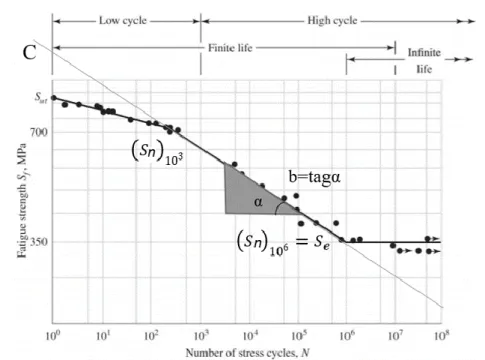
(29) Thèse de Geovana Pereira Drumond, Université de Lille, 2019. TOWARDS A PROPOSAL OF FATIGUE DAMAGE ASSESSMENT OF STEEL PIPELINES BASED ON MICROSTRUCTURAL CHANGES. fatigue strength is determined for a specified number of cycles. When a specimen does not fail even if the specified cycle is reached, test is stopped, and the corresponding stress value is marked on the curve as “runout” (given by an arrow as in Curve B). The fatigue limit in such case is assumed as 5x10⁷ cycles for design purposes.. Figure I-4: Ferrous and nonferrous S-N curves [22].. Two domains of fatigue life can be distinguished in an S-N curve (log-log scale) for steel (Figure I-5): finite life (N < 106~7 ), where the material can be under low cycle (100 < N < 103) or high cycle fatigue (N ≥ 103), and infinite life (N >106~7).. Figure I-5: S-N curve (log-log) scale for steel [22].. Low cycle fatigue (LCF) has two fundamental characteristics: plastic deformation in each cycle, and low cycle phenomenon. Fatigue tests are conducted under strain control, and the strain-life method is used for life prediction. High cycle fatigue (HCF) concerns failures corresponding to stress cycles greater than 103 cycles. In high cycle fatigue, even if stresses are elastic at the macroscopic scale, highly localized deformations are observed in the material. In this case, stresses remain globally elastic and fatigue tests can be conducted 11 © 2019 Tous droits réservés.. lilliad.univ-lille.fr.
(30) Thèse de Geovana Pereira Drumond, Université de Lille, 2019. TOWARDS A PROPOSAL OF FATIGUE DAMAGE ASSESSMENT OF STEEL PIPELINES BASED ON MICROSTRUCTURAL CHANGES. either under stress control or strain control. From design viewpoint, the main interest in engineering is for the high cycle region of S-N curve. However, low cycle fatigue data can be advantageous when only a short service life is required. In this work, the samples were tested under high cycle fatigue domain. The endurance limit For materials submitted to high-cycle fatigue, it is important to make sure that the stress level in the material is below the endurance limit, but finding this limit experimentally is time consuming because it requires testing many samples and the time for each test is relatively long. Therefore, it is usual to relate the endurance limit to other mechanical properties that are easier to determinate (such as the ultimate tensile strength, UTS) [23]. Figure I-6 shows a correlation between the ultimate strength and endurance limit, and as can be observed, for ultimate strengths up to 1400 MPa, the endurance limit seems to have a constant value. The relationship between the endurance limit and ultimate strength for steels is given in Equation I-8.. Figure I-6: Correlation between the ultimate strength and endurance limit [23].. 𝑆𝑒′ = {. 0.5 UTS 700 𝑀𝑃𝑎. 𝑓𝑜𝑟 UTS ≤ 1400 𝑀𝑃𝑎 𝑓𝑜𝑟 UTS > 1400 𝑀𝑃𝑎 Equation I-8. The prime (’) (Equation I-8) is used to denote that this value was obtained for that sample, experimentally. It is unrealistic to expect the endurance limit of a mechanical or structural equipment to match the values obtained in the laboratory [23]. Thus, some 12 © 2019 Tous droits réservés.. lilliad.univ-lille.fr.
(31) Thèse de Geovana Pereira Drumond, Université de Lille, 2019. TOWARDS A PROPOSAL OF FATIGUE DAMAGE ASSESSMENT OF STEEL PIPELINES BASED ON MICROSTRUCTURAL CHANGES. modifications factors are used to correlate the endurance limit for a given material to the value obtained from experimental tests (Equation I-9). 𝑆𝑒 = 𝑘𝑎 𝑘𝑏 𝑘𝑐 𝑘𝑑 𝑘𝑒 𝑘𝑓 𝑆𝑒′ Equation I-9. where 𝑘𝑎 = surface condition modification factor 𝑘𝑏 = size modification factor 𝑘𝑐 = load modification factor 𝑘𝑑 = temperature modification factor 𝑘𝑒 = reliability factor 𝑘𝑓 = miscellaneous-effects modification factor 𝑆𝑒′ = experimental test specimen endurance limit 𝑆𝑒 = endurance limit at the critical location of a machine part in the geometry and condition of use. Deeper explanation about each one of these k’s factors (𝑘𝑎 to 𝑘𝑓 ) can be found in [23]. The fatigue strength Besides the endurance limit, another point of the S–N curve is required to completely define the stress-life fatigue behavior [24].The S-N curve in the high cycle fatigue (103 ≤ N ≤ 106) is usually described by the Basquin equation 𝑆𝑛 = 𝐶𝑁 𝑏 , in where Sn is the fatigue strength, and the constants C (y intercept) and b (slope) are determined from the end points (𝑆𝑛 )103 and (𝑆𝑛 )106 as illustrated in Figure I-7 and as defined in Equation I-10 and Equation I-11.. 13 © 2019 Tous droits réservés.. lilliad.univ-lille.fr.
(32) Thèse de Geovana Pereira Drumond, Université de Lille, 2019. TOWARDS A PROPOSAL OF FATIGUE DAMAGE ASSESSMENT OF STEEL PIPELINES BASED ON MICROSTRUCTURAL CHANGES. Figure I-7: S-N curve plotted from results of completely reversed axial fatigue tests. Material: normalized UNS G41300 steel. Adapted from [15].. 𝐶=. (𝑆𝑛 )2103 𝑆𝑒 Equation I-10. 𝑏=−. (𝑆𝑛 )103 1 𝑙𝑜𝑔 ( ) 3 𝑆𝑒 Equation I-11. where 𝑆𝑒 is the modified endurance limit. (𝑆𝑛 )103 can be related to UTS as Equation I-12. (𝑆𝑛 )103 = 𝑓 𝑥 𝑈𝑇𝑆 Equation I-12. where f is found as Equation I-13. 𝑓=. 𝜎𝑓′ (2 𝑥 103 )𝑏 𝑈𝑇𝑆 Equation I-13. where 𝜎𝑓′ is the true stress at fracture and, for steels with Brinell hardness low than 500 (𝐻𝐵 ≤ 500), 𝜎𝑓′ is given by Equation I-14.. 14 © 2019 Tous droits réservés.. lilliad.univ-lille.fr.
(33) Thèse de Geovana Pereira Drumond, Université de Lille, 2019. TOWARDS A PROPOSAL OF FATIGUE DAMAGE ASSESSMENT OF STEEL PIPELINES BASED ON MICROSTRUCTURAL CHANGES. 𝜎𝑓′ = 𝑈𝑇𝑆 + 345 𝑀𝑃𝑎 Equation I-14. Using the equations above, the value of f is found as a function of UTS (using N=106) and it is presented graphically in Figure I-8. For ultimate tensile strength (UTS) values less than 490 MPa, f can be estimated as 0.9 to be conservative.. Figure I-8: Value of f as a function of 𝑺𝒖𝒕 [20].. If the value of f is known, the constant b can be directly found as Equation I-15. 𝑏=−. 1 𝑓 𝑥 𝑈𝑇𝑆 ) 𝑙𝑜𝑔 ( 3 𝑆𝑒 Equation I-15. And C can be rewritten as Equation I-16. (𝑓 𝑥 𝑈𝑇𝑆)2 𝐶= 𝑆𝑒 Equation I-16. I.2 FATIGUE DAMAGE IN HIGH CYCLE FATIGUE Cumulative fatigue damage (CFD) analysis still plays a key role in predicting the life of components and structures subjected to field-load histories. Fatigue damage is fundamentally a result of material structural changes at the microscopic level, such as dislocations of the atomic structures [25]. In general, three stages of damage mechanisms can be distinguished during the. 15 © 2019 Tous droits réservés.. lilliad.univ-lille.fr.
(34) Thèse de Geovana Pereira Drumond, Université de Lille, 2019. TOWARDS A PROPOSAL OF FATIGUE DAMAGE ASSESSMENT OF STEEL PIPELINES BASED ON MICROSTRUCTURAL CHANGES. process of high cycle fatigue of a sample initially without cracks. These three stages can be successively identified as microcrack initiation and microcracking (Stage I), macrocrack propagation (Stage II) and final fracture (Stage III) [26]. Stage I crack growth (microcracking) occurs along crystallographic slip bands and is dominated by shear. Stage II crack growth (macrocrack propagation) is associated with crack propagation on a plane normal to the direction of the maximum tensile principal stress attained. Stage II takes place up to a critical length of the crack is attained and the stress intensity reaches a critical value, when the crack becomes unstable with acceleration of crack propagation, and rupture occurs after few cycles in Stage III [26-30]. Figure I-9 schematically represents stages I and II of fatigue crack growth, and final fracture at 45° to the surface.. Figure I-9:Schema of stages I and II of fatigue crack growth in an AlZnMg alloy [15].. The macrocrack phase of the fatigue phenomenon (Stages II and III) have been extensively studied for decades in different materials, evidencing some common features in the behaviour of the crack propagation [26]. Numerous analytical empiric and semi-empiric models were developed to predict the fatigue crack increase in materials based on the relation of the crack growth rate and fatigue loading parameters, such as the Paris law based totally at the linear elastic fracture mechanics (LEFM) approach [31]. However, this approach is more suitably applied for modeling the fatigue crack propagation in Stage II, when the crack growth is regular and stable. However, in Stage I, the modeling of the fatigue crack growth behavior wishes a deeper knowledge of the microstructural 16 © 2019 Tous droits réservés.. lilliad.univ-lille.fr.
(35) Thèse de Geovana Pereira Drumond, Université de Lille, 2019. TOWARDS A PROPOSAL OF FATIGUE DAMAGE ASSESSMENT OF STEEL PIPELINES BASED ON MICROSTRUCTURAL CHANGES. mechanisms [26]. As the objective of the present work is to predict fatigue life of steel structures submitted to high cyclic loads before macroscopic cracking, it is of fundamental importance to better understand the mechanisms involved in the Stage I (nucleation and microcrack propagation), which is better detailed as follows. I.2.1 MICROCRACK NUCLEATION In this phase, intense deformation is observed at grains favorably oriented to shear slip and relatively less confined due to proximity to the surface, grains close to a local geometrical discontinuity (stress concentration), or grains affected by stress-corrosion effects. Figure I-10 schematically illustrates atomic rearrangements that accompany the motion of an edge dislocation as it moves in response to an applied shear stress. Dislocations are then arranged along dense crystalline planes giving rise to bands with high localized strain, called persistent slip bands (PSBs) [32], as schematically represented in Figure I-11. PSBs multiply and interact with cycling. Sequential slip of adjacent PSBs results in the development of intrusions and extrusions [33], which act as initiation sites for microcracks. A model for the mechanism of development of slip band extrusions and intrusions was proposed by Wood [34], considering that slip bands are the result of a systematic buildup of free slip movements (of the order of 1 nm). This model is schematically illustrated in Figure I-12, where the fine structure of a slip band is represented at magnifications obtainable with electron microscope. The back-and-forth fine slip movements build up notches (Figure I-12(b)) or ridges (Figure I-12(c)) at the surface, which act as stress raisers and initiation sites for microcracks. The basic premise of this model is that repeated cycling of the material leads to different amounts of net slip on different slip planes. The irreversibility of shear displacements along slip bands then results in roughening of the material surface and gradual development of a notch-ridge surface morphology. The “micro-notches” act as stress raisers and promotes additional slip [15].. 17 © 2019 Tous droits réservés.. lilliad.univ-lille.fr.
(36) Thèse de Geovana Pereira Drumond, Université de Lille, 2019. TOWARDS A PROPOSAL OF FATIGUE DAMAGE ASSESSMENT OF STEEL PIPELINES BASED ON MICROSTRUCTURAL CHANGES. Figure I-10: Atomic rearrangements that accompany the motion of an edge dislocation as it moves in response to an applied shear stress. Adapted from [15].. Figure I-11: Damage mechanism of development of a persistent slip band (PSB) and an irreversible step at the surface. Adapted from [15].. (a). (b). (c). Figure I-12: Model for the mechanism of formation of slip band extrusions and intrusions proposed by Wood [78]. (a) Static deformation. (b) Cyclic deformation leading t surface notch (intrusion) and (c) surface ridge (extrusion). Adapted from [15].. I.2.2 MICROCRACK PROPAGATION After initiation, microcracks propagate gradually into the grains along persistent slip bands. In a polycrystalline metal, the crack may extend for only a few grain diameters before crack propagation changes to the next phase (macrocrak propagation). The rate of microcrack propagation is generally very low, on the order of nm/cycle, compared to crack 18 © 2019 Tous droits réservés.. lilliad.univ-lille.fr.
(37) Thèse de Geovana Pereira Drumond, Université de Lille, 2019. TOWARDS A PROPOSAL OF FATIGUE DAMAGE ASSESSMENT OF STEEL PIPELINES BASED ON MICROSTRUCTURAL CHANGES. propagation rates (on the order of µm/cycle). Microcrack propagation is limited to the nearsurface zone of the material. Microcracks are frequently interrupted at grain boundaries that they cannot easily overcome, when adjacent grains are not favorably oriented. Microcracks are very difficult to be detected by nondestructive evaluation (NDE) techniques [15].. 19 © 2019 Tous droits réservés.. lilliad.univ-lille.fr.
(38) Thèse de Geovana Pereira Drumond, Université de Lille, 2019. CHAPTER II. INDENTATION HARDNESS. © 2019 Tous droits réservés.. lilliad.univ-lille.fr.
(39) Thèse de Geovana Pereira Drumond, Université de Lille, 2019. TOWARDS A PROPOSAL OF FATIGUE DAMAGE ASSESSMENT OF STEEL PIPELINES BASED ON MICROSTRUCTURAL CHANGES. CHAPTER II.. INDENTATION HARDNESS. This chapter is divided in two parts. The first part comprises a review of indentation hardness tests, focusing in instrumented cyclic microindentation tests, which are one of the methods used in this work to characterize microstructural changes in the material. The second part deals with microindentation testing applied to fatigue damage assessment, showing a literature review in the theme.. The hardness of a solid material can be defined as a measure of its resistance to a permanent shape change when a constant compressive force is applied. The deformation can be produced by different mechanisms, like indentation, scratching, cutting, mechanical wear, or bending. In metals, ceramics, and most of polymers, the hardness is related to the plastic deformation of the surface. Hardness has also a close relation to other mechanical properties like strength, ductility, and fatigue resistance, and therefore, hardness testing can be used in the industry as a simple, fast, and relatively cheap material quality control method [35]. Nowadays it is known that material hardness is a multifunctional physical property depending on a large number of internal and external factors.. II.1 MICROINDENTATION HARDNESS TESTING The first indentation hardness test was done by Johann Brinell in 1900 [36]. In this test, for a typical situation, a steel ball of diameter 0.39in is used to indent the material through the application of a load of 29.4kN. For soft or really hard materials, the load value is changed. Years later, in 1919, the Rockwell [37] test was introduced, and it has become the most common hardness test in use in the US. This test could be conducted rapidly because the depth of the indentation was detected by the instrument rather than the operator measuring the indentation. For the Vickers test, developed in 1925, a square-based diamond indenter was chosen with an angle of 136° between opposite faces in order to obtain hardness numbers similar in magnitude to Brinell numbers. Development of the light load Vickers test in 1932 and the Knoop test by the National Bureau of Standards in 1939 has made microindentation testing a routine procedure. Both of these tests use precisely shaped diamond indenters and various loads to determine the hardness of a wide variety of materials. The term microhardness is commonly used in place of microindentation hardness; 21 © 2019 Tous droits réservés.. lilliad.univ-lille.fr.
Figure
![Figure II-14: Influence of material constants on the threshold of stress intensity factor for high hardness steels [53].](https://thumb-eu.123doks.com/thumbv2/123doknet/3533245.103437/57.892.122.787.890.1066/figure-influence-material-constants-threshold-stress-intensity-hardness.webp)
![Figure III-4: Effects of lattice deformation on XRD peaks for (a) nondeformed material, (b) uniform deformation (macrostresses), and (c) nouniform deformation (microdeformations) [15]](https://thumb-eu.123doks.com/thumbv2/123doknet/3533245.103437/63.892.271.645.756.1101/effects-deformation-nondeformed-deformation-macrostresses-nouniform-deformation-microdeformations.webp)
![Figure III-17: Change of half value breadth with number of cycles: (a) Al phase; (b) SiC phase [97]](https://thumb-eu.123doks.com/thumbv2/123doknet/3533245.103437/78.892.142.786.232.519/figure-change-value-breadth-number-cycles-phase-phase.webp)
+7
![Figure III-18: Change of full width at half maximum with number of stress cycles: (a) aluminum phase; (b) SiC phase [98]](https://thumb-eu.123doks.com/thumbv2/123doknet/3533245.103437/79.892.143.778.125.430/figure-change-width-maximum-number-stress-cycles-aluminum.webp)
Documents relatifs
