Ministry of Higher Education and Scientific Research Colonel Ahmed Draia University of Adrar
Faculty of Sciences and Technology
Department of Mathematics and Computer Science
A Thesis Presented to Fulfill the Partial Requirement for Master’s Degree
in Computer Science
Option: Networks and Intelligent Systems
Title
Enhancement of DCT-based Image
Compression using Trigonometric Functions
Prepared by
Mohammed Lotfi Hachemi
Supervised by
Dr. Mohammed OMARI
ii
ABSTRACT
With the explosion use of multimedia in this millennium, image compression became indispensable for information technology users. It is a class of techniques that comes to efficiently store and transmit images while maintaining the best possible quality. There are several software and methods that respond to this problem of compression by maintaining a good balance between compression ratio and reconstructed image quality. In this thesis, we present an approach that uses trigonometric functions combined with the famous DCT transform. Our aim is to best utilize the sine and cosine reductive property and explore it better to gain more compression. Our experimental results showed a clear enhancement over the original DCT. Moreover, our method outperforms JPEG and JPEG2000 in terms of compression ratio as well as the PSNR.
Keywords: lossy image compression, DCT, trigonometric functions, compression
iii
ACKNOWLEDGMENTS
I would like to express my gratitude to my supervisor Dr. Mohammed OMARI for the useful comments, remarks and engagement through the learning process of this master thesis. Furthermore, I would like to thank him for introducing me to the topic as well as for the support throughout my research.
My gratitude goes to all the faculty members of our mathematical and computer science department for their continuous help during the last five years. My thanks go to the defense jury: Mr. Mohamed Amine CHERAGUI, Mr. Mohamed KOHILI and Mr. Salah YAICHI for accepting to examine my modest work.
My thanks also go to my colleagues of the mathematical and computer science department for the nice scientific and social work we did together during our bachelor’s as well as our master’s degree studies.
iv
DEDICATION
I would like to dedicate this work to My mother and father
My beloved wife and children My sisters and brothers
My big family
v
TABLE OF CONTENTS
ABSTRACT ... ii ACKNOWLEDGMENTS ... iii DEDICATION ... iv TABLE OF CONTENTS ... vLIST OF TABLES ... vii
LIST OF FIGURES ... viii
INTRODUCTION ... 1
CHAPTER 1 GENERAL SCHEME OF IMAGE COMPRESSION ... 2
INTRODUCTION ... 2
1. Digital Image ... 2
2. Image compression ... 4
3. Types of compression ... 6
4. Error Metrics ... 7
5. Image compression techniques ... 7
6. Lossless Compression Techniques ... 8
7. Lossy Compression Methods ... 10
CONCLUSION ... 13
CHAPTER 2 INNOVATIVE WORKS: IMAGE COMPRESSION ... 14
INTRODUCTION ... 14
1. JPEG – Joint Picture Expert Group ... 14
2. JPEG2000 ... 21
CONCLUSION ... 27
CHAPTER 3 A MATHEMATICAL BACKGROUND: DCT, DST AND TRIGONOMETRIC FUNCTIONS ... 28
vi
1. Discrete Cosine and Sine Transforms ... 29
2. Trigonometric functions ... 33
CONCLUSION ... 40
CHAPTER 4 DCT BASED COMPRESSION: APPLICATION OF ARCSINE TRANSFORM ... 41
INTRODUCTION ... 41
1. Proposed method with only DCT ... 41
2. Proposed method with DCT and arcsine function ... 42
3. Example of treatment of one bloc with DCT-Arcsine method. ... 44
4. Lossless compression phase ... 47
5. The application ... 48
6. Results and interpretation ... 51
CONCLUSION ... 55
CONCLUSION ... 57
vii
LIST OF TABLES
Table 1: Some famous file formats ... 4 Table 2: Table of the category and bit-coded values ... 20 Table 3: Obtained results with proposed method. ... 54 Table 4: Comparison between JPEG, JPEG2000 and proposed method results. .... 55
viii
LIST OF FIGURES
Figure 1: The pixel: is thus the smallest component of a digital image ... 3
Figure 2: DCT-Based Encoder Processing Steps ... 12
Figure 3: DCT-Based Decoder Processing Steps ... 13
Figure 4: The Encoder model of JPEG compression standard ... 15
Figure 5: The Decoder model of JPEG compression standard ... 15
Figure 6: The zigzag scan order ... 19
Figure 7: Differential coding ... 19
Figure 8: The JPEG2000 encoding and decoding process ... 22
Figure 9: Tiling, DC-level shifting, color transformation (optional) and DWT for each image component. ... 23
Figure 10: Dyadic decomposition. ... 24
Figure 11: Example of Dyadic decomposition. ... 25
Figure 12: Example of Dyadic decomposition. ... 27
Figure 13: Right triangle. ... 34
Figure 14: Sine function graph ... 35
Figure 15: Cosine function graph ... 35
Figure 16: Tangent function graph ... 36
Figure 17: Unit circle definition of sine function ... 37
Figure 18: Most commonly used angles and points of the unit circle. ... 37
Figure 19: Arcsine function graph ... 39
Figure 20: Arccosine function graph ... 39
Figure 21: Arctangent function graph ... 40
ix
Figure 23: Decompression phase with inverse DCT only... 42
Figure 24: Decompression phase with inverse DCT ans sine functions. ... 43
Figure 25: Compression phase with DCT and arcsine function. ... 43
Figure 26: Application home page. ... 49
Figure 27: Browsing for image. ... 49
Figure 28: Compressing an image. ... 50
Figure 29: Compressed image, original image and results. ... 50
Figure 30: Baboon Color 512X512 ... 51
Figure 31: Sailboat on lake Color 512X512 ... 51
Figure 32: Lena Color 512X512 ... 51
Figure 33: Peppers Color 512X512 ... 51
Figure 34: Splash Color 512X512 ... 51
Figure 35: House Color 256X256 ... 51
1
INTRODUCTION
Image compression is the science of minimizing the size in bytes of a graphics file without degrading the quality of the image to an unacceptable level. The reduction in file size allows more images to be stored in a disk or memory space. It also reduces the time required for images to be sent over the Internet or to be downloaded from web pages.
In the literature, there are several methods of image compression that claim good results in terms of reconstructed image quality. But with the rapid development of Internet, the need of creating methods of more efficiency is always necessary.
Trigonometric functions are widely used in the compression domain. In fact the discrete cosine transform (DCT) is much known as good compressor in the domain of images. In this work, we propose an enhancement of DCT using trigonometric functions such as sine and arcsine.
This thesis is organized as follow:
Chapter 1 presents image compression in general skim, and its categories. Chapter 2 explains the principle of two known methods, which are JPEG and JPEG2000.
Chapter 3 gives a mathematical definition of some trigonometric functions such as, DCT, DST, sine, cosine, arcsine, arccosine functions.
Chapter 4 exposes the proposed method, and presents its results along with a comparison with famous compressors JPEG and JPEG2000 results.
At the end, this thesis is concluded by a general conclusion and some perspectives.
2
CHAPTER 1
GENERAL SCHEME OF IMAGE COMPRESSION
INTRODUCTION
Images are important documents today; to work with them in some applications there is need to be compressed. In other words, using the data compression, the size of a particular file can be reduced. This is very useful when processing, storing or transferring a huge file, which needs lots of resources.
Image compression addresses the problem of reducing the amount of information required to represent a digital image. It is a process intended to yield a compact representation of an image, thereby reducing the image storage transmission requirements. There are two major categories of compression algorithms: lossy and lossless.
In this chapter we present the general scheme of image compression and some common compression algorithms, which include both lossless and lossy methods.
1.
Digital Image
1.1 Definition
A digital image is represented by a two-dimensional array of pixels, which are arranged in rows and columns. Hence, a digital image can be presented as M×N array (Rfael & Richard, 2002).
𝐼𝑚𝑎𝑔𝑒 = [
𝑓(0, 0) ⋯ 𝑓(0, 𝑁 − 1)
⋮ ⋱ ⋮
3
Where f (0, 0) is a function that gives the pixel of the left top corner of the array that represents the image and f (M-1, N-1) represents the right bottom corner of the array. A Grey-scale image, also referred to as a monochrome image contains the values ranging from 0 to 255, where 0 is black, 255 is white and values in between are shades of grey. In color images, each pixel of the array is constructed by combining three different channels (RGB) which are R=red, G=green and B=blue. Each channel represents a value from 0 to 255. In digital image, each pixel is stored in three bytes, while in a Grey image is represented by only one byte. Therefore, color images take three times the size of Gray images (Firas A. Jassim, October 2012).
1.2 The pixel concept
An image consists of a set of points called pixels (the word pixel is an abbreviation of PICtureELement) the pixel is thus the smallest component of a digital image. The entire set of these pixels is contained in a two-dimensional table constituting the image:
Figure 1: The pixel: is thus the smallest component of a digital image
Since screen-sweeping is carried out from left to right and from top to bottom, it is usual to indicate the pixel located at the top left hand corner of the image using the coordinates [0,0], this means that the directions of the image axes are the following:
4
The direction of the Y-axis is from top to bottom, contrary to the conventional notation in mathematics, where the direction of the Y-axis is upwards.
1.3 Types of file formats
There are a great number of file formats. The most commonly used graphic file formats are the following (THON, 2013-2014):
Table 1: Some famous file formats
Format Compression Maximum
dimensions
Maximum number of colors
BMP None /RLE 65536 x 65536 16777216
GIF LZW 65536 x 65536 256
IFF None /RLE 65536 x 65536 over 16,777,216
JPEG JPEG 65536 x 65536 over 16,777,216
PCX None /RLE 65536 x 65536 16 ,777,216
PNG RLE 65536 x 65536 over 16,777,216
TGA None /RLE 65536 x 65536 over 16,777,216
TIFF/TIF
Packbits / CCITT G3&4 / RLE / JPEG
/LZW / UIT-T
232 -1 over 16,777,216
2.
Image compression
Image compression addresses the problem of reducing the amount of information required to represent a digital image. It is a process intended to yield a compact representation of an image, thereby reducing the image storage transmission requirements. Every image will have redundant data. Redundancy means the duplication of data in the image. Either it may be repeating pixel across the image or pattern, which is repeated more frequently in the image. The image compression occurs by taking benefit of redundant information of in the image. Reduction of redundancy provides helps to achieve a saving of storage space of an image. Image compression is achieved when one or more of these redundancies are reduced or eliminated. In image compression, three basic data redundancies can be
5
identified and exploited. Compression is achieved by the removal of one or more of the three basic data redundancies (Gaurav, Sanjay, & Rajeev, October 2013).
A. Inter Pixel Redundancy
In image neighboring pixels are not statistically independent. It is due to the correlation between the neighboring pixels of an image. This type of redundancy is called Inter-pixel redundancy. This type of redundancy is sometime also called spatial redundancy. This redundancy can be explored in several ways, one of which is by predicting a pixel value based on the values of its neighboring pixels. In order to do so, the original 2-D array of pixels is usually mapped into a different format, e.g., an array of differences between adjacent pixels. If the original image pixels can be reconstructed from the transformed data set the mapping is said to be reversible (Wei, 2006).
B. Coding Redundancy
Consists in using variable length code words selected as to match the statistics of the original source, in this case, the image itself or a processed version of its pixel values. This type of coding is always reversible and usually implemented using lookup tables. Examples of image coding schemes that explore coding redundancy are the Huffman codes and the arithmetic coding technique.
C. Psycho Visual Redundancy
Many experiments on the psycho physical aspects of human vision have proven that the human eye does not respond with equal sensitivity to all incoming visual information; some pieces of information are more important than others. Most of the image coding algorithms in use today exploit this type of redundancy, such as the Discrete Cosine Transform (DCT) based algorithm at the heart of the JPEG encoding standard.
6
3.
Types of compression
The following section takes a closer look at lossy and lossless compression techniques. (Gaurav, Sanjay, & Rajeev, October 2013).
In the case of video, compression ratio causes some information to be lost; some information at a detailed level is considered not essential for a reasonable reproduction of scene. This type of compression is called lossy compression, audio compression on the other hand is not lossy, and it is called loss less compression.
3.1 Lossless Compression
In lossless compression scheme, the reconstructed image after compression is numerically identical to original image. However lossless compression can only achieve a modest amount of compression. Lossless coding guaranties that the decompressed image is absolutely identical to the image before compression.
This is an important requirement for some application domain, e.g. medical imaging, where not only high quality is in demand but unaltered archiving is a legal requirement. Lossless technique can also be used for the compression of other data types where loss of information is not acceptable, e.g. text document and program executable.
3.2 Lossy Compression
Lossy is a term applied to data compression technique in which some amount of the original data is lost during the compression process. Lossy image compression applications attempt to eliminate redundant or unnecessary information in terms of what the human eye can perceive. An image reconstructed following lossy compression contains degradation relative to the original image. Often this is because the compression scheme completely discards redundant information. However, lossy scheme are capable of achieving much higher compression. Under normal viewing condition, no visible loss is perceived (visually lossless). Lossy image data compression is useful for application to the world wide images for quicker transfer across the internet. An image reconstructed following
7
lossy compression contains degradation relative to the original. Often this is because the compression scheme completely discards the redundant information.
4.
Error Metrics
Two of the error metrics used to compare the various image compression techniques are Mean Square Error (MSE) and Peak Signal to Noise Ratio (PSNR). The MSE is the cumulative squared error between the compressed and the original image, whereas PSNR is a measure of the peak error. if you find a compression scheme having a lower MSE (and a high PSNR), you can recognize that it is a better one.
The mathematical formulae for the two are (Yusra & Chen, 2012):
𝑀𝑆𝐸 = 1 𝑚𝑛∑ ∑[𝐼(𝑖, 𝑗) − 𝐾(𝑖, 𝑗)]2 𝑛−1 𝑗=0 𝑚−1 𝑖=0 𝑃𝑆𝑁𝑅 = 10𝑙𝑜𝑔10( 𝑠2 𝑀𝑆𝐸) (𝑑𝐵)
Where I is the original image, K is the approximated version (which is actually the decompressed image) and m and n are the dimensions of the images and S is a maximum pixel value. A lower value for MSE means lesser error, and as seen from the inverse relation between the MSE and PSNR, this translates to a high value of PSNR. Logically, a higher value of PSNR is good because it means that the ratio of Signal to Noise is higher. Here, the 'signal' is the original image, and the 'noise' is the error in reconstruction. So, if you find a compression scheme having a lower MSE (and a high PSNR), you can recognize that it is a better one.
5.
Image compression techniques
On the bases of our requirements image compression techniques are broadly bifurcated in following two major categories.
8
Lossy image compression
6.
Lossless Compression Techniques
Lossless compression reduces the image size by encoding all the information from the original file, so when the image is decompressed, it will be exactly identical to the original image. There are several algorithms and techniques proposed in this filed, we can present the most popular one.
6.1 RLE Compression
Run-length encoding (RLE) is a very simple form of image compression in which runs of data are stored as a single data value and count, rather than as the original run. It is used for sequential data and it is helpful for repetitive data (Sonal, 2015). In this technique replaces sequences of identical symbol (pixel), called runs. The Run length code for a gray-scale image is represented by a sequence {Vi, Ri} where Vi is the intensity of pixel and Ri refers to the number of consecutive pixels with the intensity Vi. This is most useful on data that contains many such runs for example, simple graphic images such as icons, line drawings, and animations. It is not useful with files that don't have many runs as it could greatly increase the file size. Run-length encoding performs lossless image compression (Chen & Chuang, 2010). Run length encoding is used in fax machines.
65 65 65 70 70 70 70 62 62 62
{65,3} {70,4} {62,3}
6.2 Huffman Encoding
In computer science and information theory, Huffman coding is an entropy encoding algorithm used for lossless data compression. It was developed by Huffman. Huffman coding today is often used as a "back-end" to some other
9
compression methods (Mridul, Mathur, Loonker, & Saxena, 2012). The term refers to the use of a variable-length code table for encoding a source symbol where the variable-length code table has been derived in a particular way based on the estimated probability of occurrence for each possible value of the source symbol. The pixels in the image are treated as symbols. The symbols which occur more frequently are assigned a smaller number of bits, while the symbols that occur less frequently are assigned a relatively larger number of bits. Huffman code is a prefix code. This means that the (binary) code of any symbol is not the prefix of the code of any other symbol.
6.3 Arithmetic Coding
Arithmetic coding is a form of entropy encoding used in lossless data compression. Normally, a string of characters such as the words "hello there" is represented using a fixed number of bits per character, as in the ASCII code. When a string is converted to arithmetic encoding, frequently used characters will be stored with little {65,3} {70,4} {72,3} bits and not-so-frequently occurring characters will be stored with more bits, resulting in fewer bits used in total. Arithmetic coding differs from other forms of entropy encoding such as Huffman coding in that rather than separating the input into component symbols and replacing each with a code, arithmetic coding encodes the entire message into a single number (Jagadish & Lohit, 2012).
6.4 LZW Coding
LZW is the LempelZivWelch algorithm created in 1 984 by Terry Welch. It is the most commonly used derivative of the LZ78 family, despite being heavily patent encumbered. LZW improves on LZ78 in a similar way to LZSS; it removes redundant characters in the output and makes the output entirely out of pointers. It also includes every character in the dictionary before starting compression, and employs other tricks to improve compression such as encoding the last character of every new phrase as the first character of the next phrase. LZW is commonly found in the Graphics Interchange Format, as well as in the early specifications of the ZIP
10
format and other specialized applications. LZW is very fast, but achieves poor compression compared to most newer algorithms and some algorithms are both faster and achieve better compression (Bell, Witten, & Cleary, 1989).
7.
Lossy Compression Methods
Lossy compression techniques involve some loss of information, and data cannot be recovered or reconstructed exactly. In some applications, exact reconstruction is not necessary. For example, it is acceptable that a reconstructed video signal is different from the original as long as the differences do not result in annoying artifacts. However, we can generally obtain higher compression ratios than is possible with lossless compression. Lossy image compression techniques include following schemes:
7.1 Vector Quantization
Vector Quantization (VQ) is a lossy compression method. It uses a codebook containing pixel patterns with corresponding indexes on each of them. The main idea of VQ is to represent arrays of pixels by an index in the codebook. In this way, compression is achieved because the size of the index is usually a small fraction of that of the block of pixels.
The main advantages of VQ are the simplicity of its idea and the possible efficient implementation of the decoder. Moreover, VQ is theoretically an efficient method for image compression, and superior performance will be gained for large vectors. However, in order to use large vectors, VQ becomes complex and requires many computational resources (e.g. memory, computations per pixel) in order to efficiently construct and search a codebook. More research on reducing this complexity has to be done in order to make VQ a practical image compression method with superior quality (Sayood, 2000).
11
7.2 Predictive Coding
Predictive coding has been used extensively in image compression. Predictive image coding algorithms are used primarily to exploit the correlation between adjacent pixels. They predict the value of a given pixel based on the values of the surrounding pixels. Due to the correlation property among adjacent pixels in image, the use of a predictor can reduce the amount of information bits to represent image.
This type of lossy image compression technique is not as competitive as transform coding techniques used in modern lossy image compression, because predictive techniques have inferior compression ratios and worse reconstructed image quality than those of transform coding (Sayood, 2000).
7.3 Fractal Compression
The application of fractals in image compression started with M.F. Barnsley and A. Jacquin (Barnsley & et.al, 1988). Fractal image compression is a process to find a small set of mathematical equations that can describe the image. By sending the parameters of these equations to the decoder, we can reconstruct the original image.
7.4 Transform Based Image Compression
The basic encoding method for transform based compression works as follows:
1. Image transform: Divide the source image into blocks and apply the transformations to the blocks.
2. Parameter quantization: The data generated by the transformation are quantized to reduce the amount of information. This step represents the information within the new domain by reducing the amount of data. Quantization is in most cases not a reversible operation
3. Encoding: Encode the results of the quantization. This last step can be error free by using Run Length encoding or Huffman coding. It can
12
also be lossy if it optimizes the representation of the information to further reduce the bitrate.
Transform based compression is one of the most useful applications. Combined with other compression techniques, this technique allows the efficient transmission, storage, and display of images that otherwise would be impractical (Gu.H, 2000).
7.5 JPEG-DCT
JPEG-DCT is a transform coding method comprising four steps. The source image is first partitioned into sub-blocks of size 8x8 pixels in dimension. Then each block is transformed from spatial domain to frequency domain using a 2-D DCT basis function. The resulting frequency coefficients are quantized and finally output to a lossless entropy coder (Wallace & et.al, 1991).
Lossy JPEG encoding process is shown inFigure 2.
Figure 2: DCT-Based Encoder Processing Steps
13
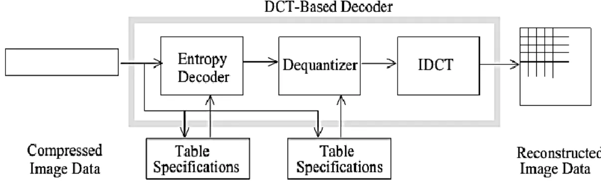
Figure 3: DCT-Based Decoder Processing Steps
CONCLUSION
In this chapter we present the general scheme of image compression and different types of image compression techniques. We can summary the chapter as follow:
Image compression is an application of data compression that attempt to reduce the redundancy of the image to be stored or transmit in an efficient form. Basically image compression techniques classified into two classes: Lossy compression techniques and lossless compression techniques. As the name indicates Lossless compression reduces the number of bits required to represent an image such that the reconstructed image is numerically identical to the original one on a pixel-by-pixel basis. On the other hand, lossy compression schemes allow degradations in the reconstructed image in exchange for a reduced bit rate. These degradations may or may not be visually apparent, and greater compression can be achieved by allowing more degradation.
14
CHAPTER 2
INNOVATIVE WORKS: IMAGE COMPRESSION
INTRODUCTION
Uncompressed image requires more space for storage and over bandwidth to transmit. For this reason, image compression addresses the problem of reducing the amount of information required to represent a digital image. It is a process intended to yield a compact representation of an image, thereby reducing the image storage transmission requirements.
To achieve these requirements, several image compression techniques have been proposed, some of these proposals have a greater success such as JPEG.
In this chapter, we will introduce the fundamental theory of two well-known image compression standards –JPEG and JPEG2000.
1.
JPEG – Joint Picture Expert Group
For the past few years, a joint ISO/IEC 10918 committee known as JPEG (Joint Photographic Experts Group) has been working to establish the first international compression standard for continuous-tone still images, both grayscale and color. JPEG’s proposed standard aims to be generic and to support a wide variety of applications for continuous-tone images. To meet the differing needs of many applications, the JPEG standard includes two basic compression methods, each with various modes of operation. A DCT-based method is specified for “lossy’’ compression, and a predictive method for “lossless’’ compression. JPEG features a simple lossy technique known as the Baseline method, a subset of the other DCT-based modes of operation. The Baseline method has been by far the
15
most widely implemented JPEG method to date, and is sufficient in its own right for a large number of applications (Wallace & et.al, 1991).
Figure 4 and Error! Reference source not found. shows the Encoder and Decoder model of JPEG. We will introduce the operation and fundamental theory of each block in the following sections.
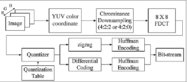
Figure 4: The Encoder model of JPEG compression standard
Figure 5: The Decoder model of JPEG compression standard
Bit-stream Dequantizer Huffman Decoding Huffman Decoding De-zigzag De-DC coding Qantization Table 8X8 IDCT Chrominance Upsampling (4:2:2 or 4:2:0) RGB Color cordinate B G R Decoded Image YUV color coordinate
16
1.1 Discrete Cosine Transform
The next step after color coordinate conversion is to divide the three color components of the image into many 8×8 blocks. The mathematical definition of the Forward DCT and the Inverse DCT are as follows:
Forward DCT:
Inverse DCT:
The f (x, y) is the value of each pixel in the selected 8×8 block, and the F(u,v) is the DCT coefficient after transformation. The transformation of the 8×8 block is also an 8×8 block composed of F (u, v). The DCT is closely related to the DFT. Both of them taking a set of points from the spatial domain and transform them into an equivalent representation in the frequency domain. However, why DCT is more appropriate for image compression than DFT? The two main reasons are:
1. The DCT can concentrate the energy of the transformed signal in low frequency, whereas the DFT cannot. According to Parseval’s theorem, the energy is the same in the spatial domain and in the frequency domain. Because the human eyes are less sensitive to the low frequency component, we can focus on the low frequency
17
component and reduce the contribution of the high frequency component after taking DCT.
2. For image compression, the DCT can reduce the blocking effect than the DFT.
After transformation, the element in the upper most left corresponding to zero frequency in both directions is the “DC coefficient” and the rest are called “AC coefficients.”
1.2 Quantization in JPEG
Quantization is the step where we actually throw away data. The DCT is a lossless procedure. The data can be precisely recovered through the IDCT (this isn’t entirely true because in reality no physical implementation can compute with perfect accuracy). During Quantization every coefficients in the 8×8 DCT matrix is divided by a corresponding quantization value. The quantized coefficient is defined in (1), and the reverse the process can be achieved by the (2).
Where Q is a quantization matrix that have the same dimension of F matrix. The goal of quantization is to reduce most of the less important high frequency DCT coefficients to zero, the more zeros we generate the better the image will compress. The matrix Q generally has lower numbers in the upper left direction and large numbers in the lower right direction. Though the high-frequency components are removed, the IDCT still can obtain an approximate matrix which is close to the original 8×8 block matrix. The JPEG committee has recommended certain Q matrix that work well and the performance is close to the optimal condition, the Q matrix for luminance and chrominance components is defined in (3) and (4).
(1) (2)
18
1.3 Zigzag Scan
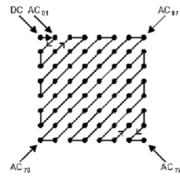
After quantization, the DC coefficient is treated separately from the 63 AC coefficients. The DC coefficient is a measure of the average value of the original 64 image samples. Because there is usually strong correlation between the DC coefficients of adjacent 8×8 blocks, the quantized DC coefficient is encoded as the difference from the DC term of the previous block. This special treatment is worthwhile, as DC coefficients frequently contain a significant fraction of the total image energy. The other 63 entries are the AC components. They are treated separately from the DC coefficients in the entropy coding process.
(3)
19
Figure 6: The zigzag scan order
1.4 Entropy Coding in JPEG Differential Coding:
The mathematical representation of the differential coding is: 𝐷𝑖𝑓𝑓𝑖 = 𝐷𝐶𝑖 = 𝐷𝐶𝑖−1 (5)
Figure 7: Differential coding
We set DC0 = 0. DC of the current block DCi will be equal to DCi-1 + Diffi. Therefore, in the JPEG file, the first coefficient is actually the difference of DCs. Then the difference is encoded with Huffman coding algorithm together with the encoding of AC coefficients.
Zero-Run-Length Coding:
After quantization and zigzag scanning, we obtain the one-dimensional vectors with a lot of consecutive zeroes. We can make use of this property and
20
apply zero-run-length coding, which is variable length coding. Let us consider the 63 AC coefficients in the original 64 quantized vectors first. For instance, we have:
57, 45, 0, 0, 0, 0, 23, 0, -30, -16, 0, 0, 1, 0, 0, 0, 0, 0, 0, 0 ... 0 (6) We encode then encode the vector (6) into vector (7).
(0,57) ; (0,45) ; (4,23) ; (1,-30) ; (0,-16) ; (2,1) ; EOB (7)
The notation (L, F) means that there are L zeros in front of F, and EOB (End of Block) is a special coded value means that the rest elements are all zeros. If the last element of the vector is not zero, then the EOB marker will not be added. On the other hand, EOC is equivalent to (0, 0), so we can express (7) as (8).
(0,57) ; (0,45) ; (4,23) ; (1,-30) ; (0,-16) ; (2,1) ; (0,0) (8)
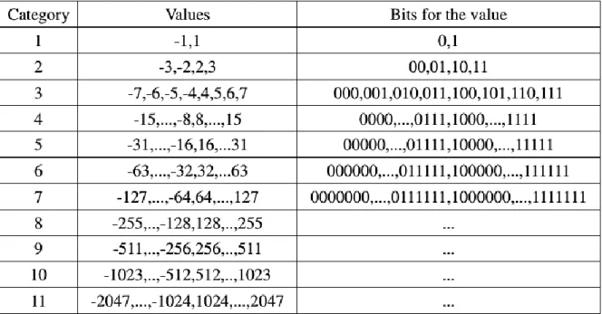
Now back to the example (2.8). The right value of the bracket is called category, and the left value of the bracket is called run. We can encode the category by looking up Table 2 which is specified in the JPEG standard. For example, 57 is in the category 6 and the bits for the value is 111001, so we encode it as 6,111001. The full encoded sequence of (6) is as (9).
(0,6,111001);(0,6,101101);(4,5,10111);(1,5,00001);(0,4,0111);(2,1,1);(0,0) (9)
21
The first two values in bracket parenthesis can be represented on a byte because of the fact that each of the two values is 0, 1, 2...15. In this byte, the higher 4-bit (run) represents the number of previous zeros, and the lower 4-bit (category) represents the value which is not 0.
The JPEG standard specifies the Huffman table for encoding the AC coefficients which is listed in table 2. The final step is to encode (9) by using the Huffman table defined in table 2.
The final step is to encode (9) by using the Huffman table. Huffman tables may be predefined and used within an application as defaults, or computed specifically for a given image in an initial statistics-gathering pass prior to compression. Such choices are the business of the applications which use JPEG; the JPEG proposal specifies no required Huffman tables.
2.
JPEG2000
JPEG2000 standards are developed for a new image coding standard for different type of still images and with different image characteristics. The coding system is intended for low bit-rate applications and exhibit rate distortion and subjective image quality performance superior to existing standards (Christopoulos, Skodras, & Ebrahimi, 2000).
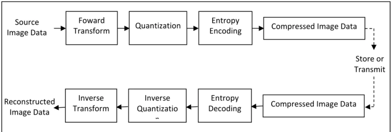
The JPEG2000 compression engine (encoder and decoder) is illustrated in block diagram form in Figure 8. The encoder, the discrete transform is first applied on the source image data. The transform coefficients are then quantized and entropy coded before forming the output code stream (bit stream). The decoder is the reverse of the encoder. The code stream is first entropy decoded, de-quantized, and inverse discrete transformed, thus resulting in the reconstructed image data. Although this general block diagram looks like the one for the conventional JPEG, there are radical differences in all of the processes of each block of the diagram.
22 Source Image Data Foward Transform Quantization Entropy
Encoding Compressed Image Data
Store or Transmit Inverse Transform Inverse Quantizatio n Entropy
Decoding Compressed Image Data
Reconstructed Image Data
Figure 8: The JPEG2000 encoding and decoding process
At the core of the JPEG2000 structure is a new wavelet based compression methodology that provides for a number of benefits over the Discrete Cosine Transformation (DCT) compression method, which was used in the JPEG lossy format. The DCT compresses an image into 8 × 8 blocks and places them consecutively in the file. In this compression process, the blocks are compressed individually, without reference to the adjoining blocks (Santa-Cruz, Ebrahimi, Ebrahimi, Askelof, Larsson, & Christopoulos, 2000). This results in “blockiness” associated with compressed JPEG files. With high levels of compression, only the most important information is used to convey the essentials of the image. However, much of the subtlety that makes for a pleasing, continuous image is lost.
In contrast, wavelet compression converts the image into a series of wavelets that can be stored more efficiently than pixel blocks. Although wavelets also have rough edges, they are able to render pictures better by eliminating the “blockiness” that is a common feature of DCT compression. Not only does this make for smoother color toning and clearer edges where there are sharp changes of color, it also gives smaller file sizes than a JPEG image with the same level of compression.
This wavelet compression is accomplished through the use of the JPEG2000 encoder (Christopoulos, Skodras, & Ebrahimi., 2000), which is pictured in Figure 8. This is similar to every other transform based coding scheme. The transform is first applied on the source image data. The transform coefficients are then quantized and
23
entropy coded, before forming the output. The decoder is just the reverse of the encoder. Unlike other coding schemes, JPEG2000 can be both lossy and lossless. This depends on the wavelet transform and the quantization applied.
The JPEG2000 standard works on image tiles. The source image is partitioned into rectangular non-overlapping blocks in a process called tiling. These tiles are compressed independently as though they were entirely independent images. All operations, including component mixing, wavelet transform, quantization, and entropy coding, are performed independently on each different tile. The nominal tile dimensions are powers of two, except for those on the boundaries of the image. Tiling is done to reduce memory requirements, and since each tile is reconstructed independently, they can be used to decode specific parts of the image, rather than the whole image. Each tile can be thought of as an array of integers in sign-magnitude representation. This array is then described in a number of bit planes. These bit planes are a sequence of binary arrays with one bit from each coefficient of the integer array. The first bit plane contains the most significant bit (MSB) of all the magnitudes. The second array contains the next MSB of all the magnitudes, continuing in the fashion until the final array, which consists of the least significant bits of all the magnitudes.
Figure 9: Tiling, DC-level shifting, color transformation (optional) and DWT for each image component.
24
Before the forward discrete wavelet transform, or DWT, is applied to each tile, all image tiles are DC level shifted by subtracting the same quantity, such as the component depth, from each sample1. DC level shifting involves moving the image tile to a desired bit plane, and is also used for region of interest coding, which is explained later. This process is pictured in Figure 9.
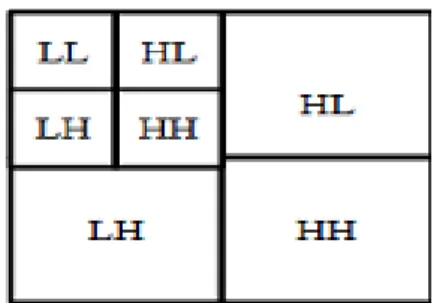
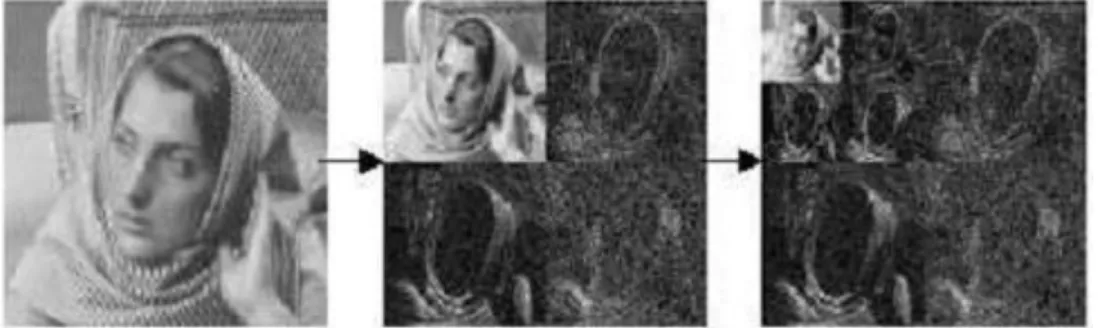
Each tile component is then decomposed using the DWT into a series of decomposition levels which each contain a number of subbands. These subbands contain coefficients that describe the horizontal and vertical characteristics of the original tile component. All of the wavelet transforms employing the JPEG2000 compression method are fundamentally one-dimensional in nature (Adams & Ward., 2001). Applying one-dimensional transforms in the horizontal and vertical directions forms two-dimensional transforms. This results in four smaller image blocks; one with low resolution, one with high vertical resolution and low horizontal resolution, one with low vertical resolution and high horizontal resolution, and one with all high resolution. This process of applying the one-dimensional filters in both directions is then repeated a number of times on the low-resolution image block. This procedure is called dyadic decomposition and is pictured in Figure 10. An example of dyadic decomposition1 into subbands with the whole image treated as one tile is shown in Figure 11.
25
Figure 11: Example of Dyadic decomposition.
To perform the forward DWT, a one-dimensional subband is decomposed into a set of low-pass samples and a set of high-pass samples. Low-pass samples represent a smaller low-resolution version of the original. The high-pass samples represent a smaller residual version of the original; this is needed for a perfect reconstruction of the original set from the low-pass set.
As mentioned earlier, both reversible integer-to-integer and nonreversible real-to real wavelet transforms can be used. Since lossless compression requires that no data be lost due to rounding, a reversible wavelet transform that uses only rational filter coefficients is used for this type of compression. In contrast, lossy compression allows for some data to be lost in the compression process, and therefore nonreversible wavelet transforms with non-rational filter coefficients can be used. In order to handle filtering at signal boundaries, symmetric extension is used. Symmetric extension adds a mirror image of the signal to the outside of the boundaries so that large errors are not introduced at the boundaries. The default irreversible transform is implemented by means of the bi-orthogonal Daubechies 9-tap/7-tap filter. The Daubechies wavelet family is one of the most important and widely used wavelet families. The analysis filter coefficients for the Daubechies 9-tap/7-tap filter (Christopoulos, Skodras, & Ebrahimi., 2000), which are used for the dyadic decomposition.
After transformation, all coefficients are quantized. This is the process by which the coefficients are reduced in precision. Dividing the magnitude of each coefficient by a quantization step size and rounding down accomplishes this. These step sizes can be chosen in a way to achieve a given level of quality. This operation
26
is lossy, unless the coefficients are integers as produced by the reversible integer 5/3 wavelet, in which case the quantization step size is essentially set to 1.0. In this case, no quantization is done and all of the coefficients remain unchanged.
Following quantization, each subband is subjected to a packet partition (Marcellin, Gormish, Bilgin, & Boliek., March 2000). Each packet contains a successively improved resolution level on one tile. This way, the image is divided into first a low quality approximation of the original, and sequentially improves until it reaches its maximum quality level. Finally, code-blocks are obtained by dividing each packet partition location into regular non-overlapping rectangles. These code-blocks are the fundamental entities used for the purpose of entropy coding.
Entropy coding is performed independently on each code-block. This coding is carried out as context-dependent binary arithmetic coding of bit planes. This arithmetic coding is done through a process of scanning each bit plane in a series of three coding passes. The decision as to which pass a given bit is coded in is made based on the significance of that bit’s location and the significance of the neighboring locations. A location is considered significant if a 1 has been coded for that location in the current or previous bit plane (Marcellin, Gormish, Bilgin, & Boliek., March 2000).
The first pass in a new bit plane is called the significance propagation pass. A bit is coded in this pass if its location is not significant, but at least one of its eight connected neighbors is significant. The second pass is the magnitude refinement pass. In this pass, all bits from locations that became significant in a previous bit plane are coded. The third and final pass is the clean-up pass, which takes care of any bits not coded in the first two passes. One significant feature of JPEG2000 is the possibility of defining regions of interest in an image. These regions of interest are coded with better quality than the rest of the image. This is done by scaling up, or DC shifting, the coefficients so that the bits associated with the regions of interest are placed in higher bit-planes. During the embedded coding process, these bits are then placed in the bit-stream before the part of the image that is not of
27
interest. This way, the region of interest will be decoded before the rest of the image. Regardless of the scaling, a full decoding of the bit-stream results in a reconstruction of the whole image with the highest possible resolution. However, if the bit-stream is truncated, or the encoding process is terminated before the whole image is fully encoded; the region of interest will have a higher fidelity than the rest of the image.
Figure 12: Example of Dyadic decomposition.
CONCLUSION
The DCT-based image compression such as JPEG performs very well at moderate bit rates; however, at higher compression ratio, the quality of the image degrades because of the artifacts resulting from the block-based DCT scheme.
Wavelet-based coding such as JPEG2000 on the other hand, provides substantial improvement in picture quality at low bit rates because of overlapping basis functions and better energy compaction property of wavelet transforms. Because of the inherent multi-resolution nature, wavelet-based coders facilitate progressive transmission of images thereby allowing variable bit rates.
28
CHAPTER 3
A MATHEMATICAL BACKGROUND: DCT, DST
AND TRIGONOMETRIC FUNCTIONS
INTRODUCTION
Applied mathematics is the branch of mathematics consists of the application of mathematical knowledge to another fields, like the use of mathematics in business, medical, industry, etc. as the title indicates DCTs, DSTs and trigonometric functions are some mathematical functions as sine, arcsine, etc. whose have some properties which can be consider useful in image compression. In this chapter we present a mathematical background of some functions that belong in this kind: we give a general mathematical presentation of the functions and some of its properties. First we present different forms of DCT and DST (Discrete Sine Transform). Then, we present the three used trigonometric functions.
29
1.
Discrete Cosine and Sine Transforms
The discrete cosine transform (DCT) and discrete sine transform (DST) are (Britanak, 2001) members of a family of sinusoidal unitary transforms. They have found applications in digital signal and image processing and particularly in transform coding systems for data compression/decompression. Among the various versions of DCT, types II and III have received much attention in digital signal processing. Besides being real, orthogonal, and separable, its properties are relevant to data compression and fast algorithms for its computation have proved to be of practical value. Recently, DCT has been employed as the main processing tool for data compression/decompression in international image and video coding standards (Rao & Hwang, Techniques and Standards for Image, Video and Audio Coding, 1996). An alternative transform used in transform coding systems is DST. In fact, the alternate use of modified forms of DST and DCT has been adopted in the international audio coding standards MPEG-1 and MPEG-2 (Moving Picture Experts Group).
1.1 The Family of DCTs and DSTs
DCTs and DSTs are members of the class of sinusoidal unitary transforms developed by Jain (Jain, 1979). A sinusoidal unitary transform is an invertible linear transform whose kernel describes a set of complete, orthogonal discrete cosine and/or sine basis functions. The well-known Karhunen–Loève transform (KLT), generalized discrete Fourier transform (Bongiovanni, Corsini, & Frosini, 1976), generalized discrete Hartley transform (Rao & Hwang, 1996) or equivalently generalized discrete W transform (Wang & Hunt, 1985), and various types of the DCT and DST are members of this class of unitary transforms.
The set of DCTs and DSTs introduced by Jain (Jain, 1979) is not complete. The complete set of DCTs and DSTs, so-called discrete trigonometric transforms, has been described by Wang and Hunt (Wang & Hunt, 1985). The family of discrete trigonometric transforms consists of 8 versions of DCT and corresponding 8 versions of DST (Martucci, 1992). Each transform is identified as even or odd and
30
of type I, II, III, and IV. All present digital signal and image processing applications (mainly transform coding and digital filtering of signals) involve only even types of the DCT and DST. Therefore, this chapter considers four even types of DCT and DST.
1.2 Definitions of DCTs and DSTs
In subsequent sections, N is assumed to be an integer power of 2, i.e. N = 2m. A subscript of a matrix denotes its order, while a superscript denotes the version number.
Four normalized even types of DCT in the matrix form are defined as DCT
𝐷𝐶𝑇 − 𝐼: [𝐶𝑁+1𝐼 ] 𝑛𝑘 = √ 2 𝑁 [𝜑𝑛𝜑𝑘𝑐𝑜𝑠 𝜋𝑛𝑘 𝑁 ] , 𝑛, 𝑘 = 0,1, … , 𝑁 𝐷𝐶𝑇 − 𝐼𝐼: [𝐶𝑁𝐼𝐼] 𝑛𝑘 = √ 2 𝑁 [𝜑𝑘𝑐𝑜𝑠 𝜋(2𝑛 + 1)𝑘 2𝑁 ] , 𝑛, 𝑘 = 0,1, … , 𝑁 − 1 𝐷𝐶𝑇 − 𝐼𝐼𝐼: [𝐶𝑁𝐼𝐼𝐼] 𝑛𝑘 = √ 2 𝑁 [𝜑𝑛𝑐𝑜𝑠 𝜋𝑛(2𝑘 + 1) 2𝑁 ] , 𝑛, 𝑘 = 0, 1, … , 𝑁 − 1 𝐷𝐶𝑇 − 𝐼𝑉: [𝐶𝑁𝐼𝑉] 𝑛𝑘 = √ 2 𝑁 [𝑐𝑜𝑠 𝜋(2𝑛 + 1)(2𝑘 + 1) 4𝑁 ] , 𝑛, 𝑘 = 0,1, … , 𝑁 − 1 Where 𝜑𝑝 = { 1 √2 𝑝 = 0 𝑜𝑟 𝑝 = 𝑁 1 𝑜𝑡ℎ𝑒𝑟𝑤𝑖𝑠𝑒
And the corresponding four normalized even types of the DST are defined as
𝐷𝑆𝑇 − 𝐼: [𝑆𝑁−1𝐼 ]𝑛𝑘 = √ 2 𝑁 [𝑠𝑖𝑛
𝜋(𝑛 + 1)(𝑘 + 1)
31 𝐷𝑆𝑇 − 𝐼𝐼: [𝑆𝑁𝐼𝐼]𝑛𝑘 = √ 2 𝑁 [𝜑𝑘𝑠𝑖𝑛 𝜋(2𝑛 + 1)(𝑘 + 1) 2𝑁 ] , 𝑛, 𝑘 = 0,1, … , 𝑁 − 1 𝐷𝑆𝑇 − 𝐼𝐼𝐼: [𝑆𝑁𝐼𝐼𝐼] 𝑛𝑘 = √ 2 𝑁 [𝜑𝑛𝑠𝑖𝑛 𝜋(𝑛 + 1)(2𝑘 + 1) 2𝑁 ] , 𝑛, 𝑘 = 0,1, … , 𝑁 − 1 𝐷𝑆𝑇 − 𝐼𝑉: [𝑆𝑁𝐼𝑉]𝑛𝑘 = √ 2 𝑁 [𝑠𝑖𝑛 𝜋(2𝑛 + 1)(2𝑘 + 1) 4𝑁 ] , 𝑛, 𝑘 = 0,1, … , 𝑁 − 1 Where: 𝜑𝑝 = { 1 √2 𝑝 = 0 𝑜𝑟 𝑝 = 𝑁 1 𝑜𝑡ℎ𝑒𝑟𝑤𝑖𝑠𝑒
The DCT-I introduced by Wang and Hunt (Wang & Hunt, The discrete cosine transform - a new version, 1983) is defined for the order 𝑁 + 1. It can be considered a special case of symmetric cosine transform introduced by Kitajima (Kitajima, 1980). The DST-I introduced by Jain (Jain, A fast Karhunen–Loève transform for a class of random processes, 1976) is defined for the order 𝑁 − 1 and constitutes the basis of a technique called recursive block coding (Jain, 1989). The DCT-II and its inverse, DCT-III, first reported by Ahmed, Natarajan, and Rao (Ahmed, Natarajan, & Rao, 1974), has an excellent energy compaction property, and among the currently known unitary transforms it is the best approximation for the optimal KLT. The DST-II and its inverse, DST-III, have been introduced by Kekre and Solanki (Kekre & Solanki, 1978). DST-II is a complementary or alternative transform to DCT-II used in transform coding. DCT-IV and DST-IV introduced by Jain (Jain, A sinusoidal family of unitary transforms Trans. on Pattern Analysis and Machine Intelligence, 1979) have found applications in the fast implementation of lapped orthogonal transform for the efficient transform/subband coding (Malvar, 1990).
32
1.3 Properties
The basic mathematical properties of discrete transforms are fundamental for their use in practical applications. Thus, properties such as scaling, shifting, and convolution are readily applied in the discrete transform domain. In the following, the most relevant mathematical properties of the family of DCTs and DSTs are briefly summarized.
DCT and DST matrices are real and orthogonal. All DCTs and DSTs are separable transforms; the multidimensional transform can be decomposed into successive application of one-dimensional (1-D) transforms in the appropriate directions.
The following relations hold for inverse DCT matrices [𝐶𝑁+1𝐼 ]−1= [𝐶 𝑁+1𝐼 ]𝑇 = [𝐶𝑁+1𝐼 ] [𝐶𝑁𝐼𝐼]−1 = [𝐶 𝑁𝐼𝐼]𝑇 = [𝐶𝑁𝐼𝐼𝐼] [𝐶𝑁𝐼𝐼𝐼]−1 = [𝐶 𝑁𝐼𝐼𝐼]𝑇 = [𝐶𝑁𝐼𝐼] [𝐶𝑁𝐼𝑉]−1 = [𝐶 𝑁𝐼𝑉]𝑇 = [𝐶𝑁𝐼𝑉] and for inverse DST matrices
[𝑆𝑁−1𝐼 ]−1 = [𝑆 𝑁−1𝐼 ]𝑇 = [𝑆𝑁−1𝐼 ] [𝑆𝑁𝐼𝐼]−1 = [𝑆 𝑁𝐼𝐼]𝑇 = [𝑆𝑁𝐼𝐼𝐼] [𝑆𝑁𝐼𝐼𝐼]−1 = [𝑆 𝑁𝐼𝐼𝐼]𝑇 = [𝑆𝑁𝐼𝐼] [𝑆𝑁𝐼𝑉]−1 = [𝑆 𝑁𝐼𝑉]𝑇 = [𝑆𝑁𝐼𝑉]
1.4 DCT use in data compression
In general, there are several characteristics that are desirable in a transform when it is used for the purpose of data compression. DCT-III, have been employed in the international image/video coding standards: JPEG for compression of still images, MPEG for compression of motion video including HDTV (High Definition Television), H.261 for compression of video telephony and teleconferencing, and
33
H.263 for visual communication over ordinary telephone lines (Rao & Hwang, 1996).
2.
Trigonometric functions
2.1 Introduction
In mathematics, the trigonometric functions (also called the circular functions) are functions of an angle. They relate the angles of a triangle to the lengths of its sides. Trigonometric functions are important in the study of triangles and modeling periodic phenomena, among many other applications. Trigonometric functions have a wide range of uses including computing unknown lengths and angles in triangles (often right triangles). Trigonometric functions are used, for instance, in navigation, engineering, and physics. A common use in elementary physics is resolving a vector into Cartesian coordinates. The sine and cosine functions are also commonly used to model periodic function phenomena such as sound and light waves, the position and velocity of harmonic oscillators, sunlight intensity and day length, and average temperature variations through the year.
In this section, we present the most central trigonometric functions such as sine, cosine, and tangent.
2.2 Right-angled triangle definitions
A right triangle is a triangle with a right angle (90°) (See Figure 13) (Adamson & Nicholas, 1998).
34
Figure 13: Right triangle.
To define the trigonometric functions for the angle A, start with any right triangle that contains the angle A. The three sides of the triangle are named as follows:
The hypotenuse is the side opposite the right angle, in this case side h. The hypotenuse is always the longest side of a right-angled triangle.
The opposite side is the side opposite to the angle we are interested in (angle A), in this case side a.
The adjacent side is the side having both the angles of interest (angle A and right-angle C), in this case side b.
2.3 Definition of sine, cosine and tangent
Sine: The sine of an angle is the ratio of the length of the opposite side to the
length of the hypotenuse. (The word comes from the Latin sinus for gulf or bay since, given a unit circle, it is the side of the triangle on which the angle opens.) (Adamson & Nicholas, 1998) In our case
Cosine: The cosine of an angle is the ratio of the length of the adjacent side
to the length of the hypotenuse: so called because it is the sine of the complementary or co-angle (Adamson & Nicholas, 1998). In our case
35
Tangent: The tangent of an angle is the ratio of the length of the opposite
side to the length of the adjacent side: so called because it can be represented as a line segment tangent to the circle, that is the line that touches the circle, from Latin lineatangens or touching line (cf. tangere, to touch) (Adamson & Nicholas, 1998). In our case
2.4 Sine, cosine and tangent graphs
Figure 14: Sine function graph
36
Figure 16: Tangent function graph
2.5 Definitions of Trigonometric Functions for a Unit Circle
In the unit circle, one can define the trigonometric functions cosine and sine as follows. If (x,y) is a point on the unit circle, and if the ray from the origin (0,0) to that point (x,y) makes an angle θ with the positive x-axis, (such that the counterclockwise direction is considered positive), then:
Cosθ = x/1 = x and Sinθ = y/1 = y
Then, each point (x,y) on the unit circle can be written as (Cosθ, Sinθ). Combined with the equation x2 + y2 = 1, the definitions above give the relationship sin2θ+cos2θ=1. In addition, other trigonometric functions can be defined in terms of x and y: tan θ = sinθ/cosθ = y/x
Figure 17 below shows a unit circle in the coordinate plane, and Figure 18
shows a unit circle in the coordinate plane with some useful values of angle θ, and the points (x, y) = (cosθ, sinθ), that are most commonly used.
37
Figure 18: Most commonly used angles and points of the unit circle.
2.6 Some properties of sine, cosine and tangent functions
sin(-θ) = -sin θ
38 cos(-θ) = cos θ
tan(-θ) = -tan θ sin2θ + cos2θ = 1 sin2θ = 2 sin θ cos θ
cos2θ = cos2θ – sin2θ = 1-2 sin2θ = 2 cos2θ -1 tan2 θ = 2 tan θ/ (1 − tan2θ)
sin A ± B = sinAcosB ± cosAsinB cos A ± B = cosAcos B ∓sinAsinB
2.7 Inverse trigonometric functions
When we studied inverse functions in
general (see Inverse Functions), we learned that the inverse of a function can be formed by reflecting the graph over the identity line y = x. We also learned that the inverse of a function may not necessarily be another function.
Look at the sine function (in red) at the right. If we reflect this function over the identity line, we will create the inverse graph (in blue). Unfortunately, this newly formed inverse graph is not a function. Notice how the green vertical line intersects the new inverse graph in more than one location, telling us it is not a function. (Vertical Line Test).
By limiting the range to see all of the y-values without repetition, we can define inverse functions of the trigonometric functions. It is possible to form inverse functions at many different locations along the graph. The functions shown here are what are referred to as the "principal" functions.
Definition: In mathematics, the inverse trigonometric functions (occasionally called cyclometric functions) (Dörrie, 1965) are the inverse functions of the trigonometric functions (with suitably restricted domains). Specifically, they are the inverses of the sine, cosine, tangent, cotangent, secant, and cosecant functions. They are used to obtain an angle from any of the angle's trigonometric
39
ratios. Inverse trigonometric functions are widely used in engineering, navigation, physics, and geometry.
Inverse sine:
notation domain range
f (x) = sin-1(x) f (x) = arcsin(x)
[-1,1]
Figure 19: Arcsine function graph
Inverse cosine:
notation domain range
f (x) = cos-1(x)
f (x) = arccos(x) [-1,1] [0, л]
Figure 20: Arccosine function graph
Inverse tangent:
notation domain range
f (x) = tan-1(x) f (x) = arctan(x)
40
Figure 21: Arctangent function graph
CONCLUSION
The DCT and sine functions have interesting properties that may cleverly be exploited for images compression. DCT condenses the image energy into a reduced set of coefficients. Sine function, on the other hand, reduces the space size in case we tackle a pretreatment of images.
41
CHAPTER 4
DCT BASED COMPRESSION: APPLICATION OF
ARCSINE TRANSFORM
INTRODUCTION
In this chapter, we will present our proposed method: Enhancement of DCT-Based Image Compression using Trigonometric Functions. As the title indicates, we suggest in our proposition a combination between DCT and arcsine function; in aim, to get better results compared with which has been got by the traditional techniques such as JPEG.
At the level of storage on the hard disc, we use the bitmap format. In the lossless compression phase, as well developed software that belongs to PAQ Algorithms family, initially promoted by Matt Mahoney, is used to optimize the compression much better.
1.
Proposed method with only DCT
1.1 Compression:
The forward processing (compression phase) is shown in Figure 22, and follows the following order: first, we divide the image into several 16x16 blocs. Next, the DCT is applied and the values which are less than 13.5 are set into zero. After normalization for the storage (values between 0 and 255), we apply the zigzag scan, like JPEG algorithm, and transform the obtained vector into a 4x64 bloc. Then, we obtain an image different in size from the original image. After that, we
42 Lossless decompressio n 4X64 Blocs Inverse
zigzag Denormalization 16X16 Blocs
Inverse DCT
Inverse
Shifting Image
Figure 23: Decompression phase with inverse DCT only.
reorganize the lines of this image, and store it into bitmap format. Finally, we apply lossless compression (Mikulic, 2001).
1.2 Decompression
The inverse path shown in Figure 23 is scanned. So, we apply lossless decompression, and divide image into 4x64 blocs. Transform the bloc into a 256 sized vector, apply inverse zigzag to obtain 16x16 bloc. Then inversed DCT is applied. The image is reset (Mikulic, 2001).
2.
Proposed method with DCT and arcsine function
2.1 Compression:
The forward processing (compression phase) is shown in Figure 25 and follows the following order: first, we divide the image into several 16x16 blocs and we normalize the bloc by dividing it by 200. Then, we apply the arcsine function and multiply by 185.4. Next, the DCT is applied and the values which are less than
Figure 22: Compression phase with DCT only.
Image 16X16 Blocs DCT Normalization Quantization Zigzag scan Blocs 4X64 Bitmap file Lossless compression Shifting
43
13.5 are set into zero. After normalization for the storage (values between 0 and 255), we apply the zigzag scan, like JPEG algorithm, and transform the obtained vector into a 4x64 bloc. Then, we obtain an image different in size from the original image. After that, we reorganize the lines of this image, and store it into bitmap format. Finally, we apply lossless compression.
2.2 Decompression
The inverse path shown in Figure 24 is scanned. So, we apply lossless decompression, and divide image into 4x64 blocs. Transform the bloc into a 256 sized vector, apply inverse zigzag to obtain 16x16 bloc. Then inversed DCT is applied and sine function with normalization is applied. The image is then restored.
Image 16X16 Blocs DCT Normalization
Quantization Zigzag
scan Blocs 4X64 Bitmap file compression Lossless Arcsine function
with normalization Shifting
Figure 25: Compression phase with DCT and arcsine function.
Figure 24: Decompression phase with inverse DCT ans sine functions. Lossless decompression Inverse zigzag Denormalization Inverse DCT
Sine function with normalization 4X64 Blocs 16X16 Blocs Inverse Shifting Image Dequantization Bitmap file
44
3.
Example of treatment of one bloc with DCT-Arcsine method.
In this example, we use a 4x4 bloc instead 16x16 bloc:75 65 72 69 59 74 69 67 67 61 67 75 71 58 62 69 3.3 Compression We shift: 160 – Bloc 85 95 88 91 101 86 91 93 93 99 93 85 89 102 98 91 We divide by 200 0.425 0.475 0.440 0.455 0.505 0.430 0.455 0.465 0.465 0.495 0.465 0.425 0.445 0.510 0.490 0.455 We apply arcsine function
0.439 0.495 0.456 0.472 0.529 0.444 0.472 0.484 0.484 0.518 0.484 0.439 0.461 0.535 0.512 0.472
45 We multiply by 185.4 81.38 91.77 84.47 87.58 98.15 82.41 87.58 89.67 89.67 96.01 89.67 81.38 85.5 99.22 94.94 87.58 We apply DCT 356.7 4.5 -6.29 -3.02 -7.06 -2.03 8.902 0.034 -0.52 -6.77 -7.89 -6.79 -3.34 1.443 -8.73 -5.78 We divide by 10 and add 92
127.7 92.45 91.37 91.7 91.29 91.8 92.89 92 91.95 91.32 91.21 91.32 91.67 92.14 91.13 91.42 We apply round function
128 92 91 92 91 92 93 92 92 91 91 91 92 92 91 91 We use the zigzag scan
128 92 91 92 92 91 92 93 91 92 92 91 92 91 91 91 We transform the obtained vector into 2x8 bloc
128 92 91 92 92 91 92 93 91 92 92 91 92 91 91 91
With many blocs, this matrix will be stored into a bitmap format and lossless compression is applied.