HAL Id: hal-00449605
https://hal.archives-ouvertes.fr/hal-00449605
Submitted on 22 Jan 2010
HAL is a multi-disciplinary open access
archive for the deposit and dissemination of
sci-entific research documents, whether they are
pub-lished or not. The documents may come from
teaching and research institutions in France or
abroad, or from public or private research centers.
L’archive ouverte pluridisciplinaire HAL, est
destinée au dépôt et à la diffusion de documents
scientifiques de niveau recherche, publiés ou non,
émanant des établissements d’enseignement et de
recherche français ou étrangers, des laboratoires
publics ou privés.
Multidisciplinary and multiobjective optimization:
Comparison of several methods
Philippe Dépincé, Benoît Guédas, Jérôme Picard
To cite this version:
Philippe Dépincé, Benoît Guédas, Jérôme Picard. Multidisciplinary and multiobjective optimization:
Comparison of several methods. 7th World Congress on Structural and Multidisciplinary
Optimiza-tion, May 2007, Seoul, South Korea. �hal-00449605�
7th
World Congress on Structural and Multidisciplinary Optimization
COEX Seoul, 21 May - 25 May 2007, Korea
Multidisciplinary and multiobjective optimization:
Comparison of several methods
Philippe D´epinc´e1
, Benoˆıt Gu´edas1
, J´erˆome Picard1,2 1
Institut de Recherche en Communications et Cybern´etique de Nantes
UMR n◦6597 CNRS, ´Ecole Centrale de Nantes, Universit´e de Nantes, ´Ecole des Mines de Nantes 1, rue de la No¨e, BP 92101, 44321 Nantes Cedex 3, France
2SIREHNA
1, rue de la No¨e, BP 42105, 44321 Nantes Cedex 3, France Abstract
Engineering design of complex systems is a decision making process that aims at choosing from among a set of options that implies an irrevocable allocation of resources. It is inherently a multidisciplinary and multi-objective process. The paper describes some classical multidisciplinary optimization (MDO) methods with their advantages and drawbacks. Some new approaches combining genetic algorithms (MOGA) and collaborative optimization (CO) are presented. They allow to: 1) increase the convergence rate when a design problem can be broken up regarding design variables, and 2) provide an optimal set of design variables in case of multi-level multi-objective design problem.
Keywords: Multidisciplinary Design Optimization, Bi-Level Collaborative Optimization, Genetic Algorithm, Pareto Frontier
1 Introduction
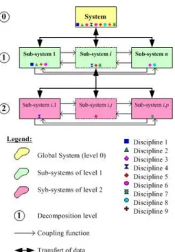
Nowadays, the designer has to face the continuous growing complexity of engineering problems (Fig. 1), but also, the increasing economic competition that have led to a specialization and distribution of knowledge, expertise, tools and work sites (Fig. 2). Consequently, multi-objective optimization (MOO) and multidisciplinary design optimization (MDO) have been more and more used to provide one solution or an optimal set of solutions. While single-discipline optimization is mature, the design and optimization of complex systems ( more than one discipline) is still quite young. Since the white papers provided in 1991 and 1998 by the AIAA [1, 2], lot of re-searches have been done in the multidisciplinary optimization domain: at the beginning centered on the aerospace industries, they are now used in different kinds of enterprise (automotive, ship building, . . . ) which search in such a tool a way to improve theirs products, organizations, . . . One of the problems is that some engineers in industry think that researchers are making a big deal out of a concept that they have always used in their work. Currently, the real-world engineering problems (in aerospace or in automotive) involve thousands of variables, hundreds of analyses and engineers, and are far more complex that the ones studied by the researchers. However, even a rocket can sent a satellite in the space, the associated systems are not fully optimized. MDO can be summarized as the development of strategies that from current analysis tools (FEA, . . . ) and optimization techniques help the engineers to take the best decision during the design process in order to obtain an optimized complex products or systems.
The first methodologies were based on classical optimization methodologies and the main point was how to manage coupling variables and the disciplinary design variables. A first classification appears based on the optimizer level (mono or bi-level). These methodologies (AAO, MDF, IDF, CO, CSSO, BLISS, . . . ) have been extensively studied. However generally the function to optimize is mono-objective and defined at the system level and the result of the optimization process is a single point.
In most cases real engineering problems are multi-objective and some disciplines can have their own objectives to optimize. The increasing of computer performance, the development of approximation methods (response surface) have permitted the development of multi-objective methodologies [3] that allow the exploration of the solution space and lead not to one single solution but to a set of non dominated solutions (Pareto frontier) which allow the designer to take a better decision while comparing several designs in an acceptable period of time.
Figure 1: Structural decomposition of a multilevel system
Figure 2: Context of the extended enterprise
As a consequence, new methods appear recently that combine multidisciplinary and multi-objective optimiza-tion methods. Some are just the applicaoptimiza-tion of multi-objective methods to the formally described MDO method-ologies. Others try to express the MDO problems not from the mathematical description of the global problem but from an engineer point of view and its way of working. Such a structure requires efficient optimization method-ologies that take into account the decomposition of the product into several disciplines that are simultaneously optimized in different structures (team, division, subcontractors) and places. This kind of structures can be con-sidered as complex systems and defined as assemblies of interacting members that are difficult to understand as a
whole[4].
A complex system can be decomposed by several ways: object, aspect, sequential and model-based [5].
Objectdecomposition divides a system by physical components. Aspect (or discipline) decomposition divides the system according to different disciplines - or specialities [6]. Object and aspect partitioning are ”natural” partitions and typically large companies employ both types of partitions simultaneously (mixed partition) in a matrix management organization. Sequential decomposition is applicable when partitioned sub-problems are organized by work-flow or process logic and presumes unidirectionality of design information.
The objectives of this paper are (i) to discuss multidisciplinary optimization methods such as MDF, IDF, AAO, CO and point out their drawbacks and (2) present methods that combine Collaborative Optimization (CO) and Genetic Algorithms (GA) and fit more the way a complex products is designed.
2 A multidisciplinary problem: definition
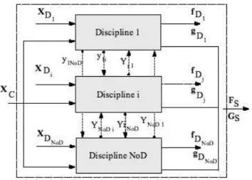
A classical way to describe a multidisciplinary problem is given by -a schema is given in Fig. 3: Find the set of design variables (DV) x ∈ DV S: x = (x1, x2, ..., xNoD, z) that minimize objective functions F ∈
OF S : F(x) = (FD1(x1, z, y1), ..., FDNoD(xNoD, z, yNoD), FS(X)) and simultaneously satisfy equality
and inequality constraints : G(x) = (GD1(x1, z), ..., GDNoD(xNoD, z), GS(x)) where N oD is the
num-ber of disciplines, N F S is the number of system functions - and N GS is the number of system constraints; xi, FDi, GDiare respectively the set of design variables, objective functions and constraint functions associated
to discipline i; z, FS, GS are respectively the set of common design variables, objective functions and
con-straint functions associated to the whole system; yi is the set of coupled functions needed to compute FDi:
In a multidisciplinary problem, each sub-system (discipline) has its own design variables, objective and constraint functions. The design variables are those we can modify in order to optimize the functions as-sociated to the discipline. Some design variables can be common to at least two sub-systems, in this case they are called common variables. The disciplinary outputs from one discipline can be needed to evaluate another sub-system. In this case there is a coupling between two disciplines, these variables will be called coupling variable [7, 8]. The third variable type, state variables, are internal variables particular to one disci-pline: they represent conditions that have to be satisfied within the discipline. Within each discipline an evalu-ation/analysis is conducted that allows to compute the outputs: functions, constraints and coupling variables if needed.
Figure 3: A fully coupled disciplines system Within the general case, the system level
objec-tives can be a function or not of the objecobjec-tives of the disciplines.
Frequently, complex systems are non-hierarchical what means that there is no reason to process the optimization of one sub-system be-fore another [8]. In the optimization process of such systems, the presence of coupling functions and their recognition constitutes a real challenge for researchers.
3 Classical methodologies: mono-level ver-sus multi-level
Most of the MDO methods reported in the literature are developed specifically for single-objective problems with continuous variables and differentiable objective. These MDO meth-ods are classified in two groups: mono-level and bi-level. The single-level (mono-level) group implies optimization at only the supervisor level.
The bi-level group allows each discipline to manage its own optimization regarding its design variables.
Generally the formulation of the MDO problem is simplified: the authors only consider a single objective function at the system level and the sub-system are used as analysers or evaluators [9, 10]. The problem can be formulate as in Eq. 1. Eq. 2 will be the example used to explain the differences between the formulation.
Minimize f (x, z, y) under variables x, z under constraints G(x, z, y)
with yi= yi(x, yj,j6=i) ∀i
(1) Minimize f (x) = x2 2+ x3+ y1+ exp(−y2) g1: 1 −3.16y1 60, g2: y242 − 1 6 0, y1= x21+ x2+ x3− 0.2 × y2 y2= √y1+ x1+ x3 (2) Problem given by Eq. 2 has 2 common variables (x1andx3) and one variable proper to system 1:x2. The
two subsystems are defined respectively thanks togiandyi. The problem can be rewritten as:
Minimize f (x, z) = x2+ z 2+ y1+ exp(−y2) g1: 1 − 3.16y1 60, g2: y242 − 1 6 0, y1= z12+ x + z2− 0.2 × y2 y2= √y1+ z1+ z2 (3) 3.1 Mono-level approaches
The mono-level family contains three multidisciplinary methods: All-At-Once (AAO), Multidisciplinary Fea-sible (MDF) and Individual Discipline FeaFea-sible (IDF) [9, 11, 12, 13]. There are some minor differences between
all the given formulations but the whole idea is always the same. In [14], Dennis et al. proposed an extension of all the above methodologies to the optimization of system of systems.
Multidisciplinary-Feasible Method (MDF) is the traditionnal, natural approach to solve a MDO problem and the most used. A complete multidisciplinary analysis is performed for each choice of the design variables by the optimizer. This is conceptually very simple, and once all disciplines are coupled to form one single multidisci-plinary analysis module, one can use the same techniques that are used in single discipline optimization.
In this formulation he optimization variables are the design variables, the optimization is global global and each iteration give a feasible solution. Moreover the evaluation within the disciplines are independant. Drawbacks are the computational effort and the non garanty of the convergence. Moreover it does not exploit the potentially weak coupling between disciplines and so does not allow several analyses modules to run in parallel.
In All-At-Once (AAO) all the variables (design, coupling, state) are considered as design variables and the analysis system equations become constraint. This allows to skip the iterative analysis of sub-system that are CPU consuming but it increases the dimension of the design space. The problem formulation can be expressed by:
Minimize f (x, z, y, s) under variables x, z, y, s under constraints G(x, z, y) yi− yi(x, yj,j6=i, s) = 0 ∀i (4) Minimize f (x) = x2+ z 2+ y1+ exp(−y2) variables x, z, y : g1: 1 − y1 3.16 60, g2: y2 24− 1 6 0, 0 = z2 1+ x + z2− 0.2 × y2− y1 0 = √y1+ z1+ z2− y2 (5) Drawbacks associated with AAO are: the number of design variables and constraint functions increases, there is no possibility to use evaluator specific to each discipline and the feasibility is not guaranty. However this method is robust and can handle large size problem.
Individual Disciplinary Feasible (IDF) is a compromise between AAO and MDF. At each point, each discipline is feasible but the whole system will only be feasible at the end. In this methodology, coupling variables are added to design variables and some auxiliary variables, u, are introduced that allows to decouple the disciplines. Some equality constraints are added that allow compatibility between coupling and auxiliary variables. This substitution relax the coupling between disciplines: for some iterations, a point can not fulfill all the coupling.
Minimize f (x, z, u) under variables x, z, u under constraints G(x, z, u) ui− yi(x, uj,j6=i) = 0 ∀i (6) Minimize f (x, z, u) = x2 + z2+ y1+ exp(−u2) variables x, z, u : g1: 1 − (u1/3.16) 6 0, g2: (u2/24) − 1 6 0, 0 = y− u, y1= z12+ x + z2− 0.2 × u2 y2= √u1+ z1+ z2 (7) One of the advantages is possibility to use legacy solver and the size of the problem is less than in AAO. Drawback is that the point are not feasible at each step.
3.2 Multi-level approaches
In the case of bi-level optimization method, the original optimization problem is divided into optimization at both system and sub-system levels. Coordination between sub-systems is managed by an optimizer in charge of solving inconsistencies between the disciplines. Several strategies have been developed and the most discussed are Collaborative Optimization (CO) [15], and Concurrent SubSpace Optimization (CSSO)[16]. Others methods like Bi-Level Integrated System Synthesis (BLISS)[17], Analytical Target Cascading (ATC) [18] or Physical Programming (PP)[19] have been developed but will not be detailed in this paper.. The two first are part of the Discipline Feasible Constraint (DFC) group. The primary features of each of these architectures include: i) the use of heterogeneous hardware or software, specific to the domain, to solve the subspace optimization problems, ii) the decomposition keeps domain-specific constraint information in the subproblem, iii) the system leaves most of the design decisions (selection of local variables) to the disciplinary groups that understand the local formulation.
In Collaborative Optimization (CO) subspace optimizers are integrated with each subsystem. Through sub-system optimization each discipline is given control over its own set of local design variables and is charged with satis-fying its own domain specific constraints. Explicit knowledge of the other groups constraints or design variables is not required. The objective of each subsystem optimizer is to agree upon the values of the interdisciplinary variables with the other groups. A system level optimizer is employed to coordinate this process while minimiz-ing the overall objective. It promotes disciplinary autonomy while achievminimiz-ing interdisciplinary compatibility. The problem can be expressed as:
• At the system level:
Minimize f (zS, yS, x∗i) under variables zS, yS under constraints J∗ i((zS, z∗i, yS, y∗(x∗i, yS, z∗i)) = 0 ∀i = 1, ..., NoD (8) whereJ∗
i represents a measure of the interdisciplinary discrepancy for theithdiscipline after solving the
disciplinary subsystem and∗represent the results from the solution of theithdiscipline optimization
prob-lem.
• At the subsystem level:
Minimize Ji((z∗S, zi, y∗S, yi(xi, yS∗, zi)) =P(z∗S− zi)2+P(yS∗− yi)2
under variables zi, xi,
under constraints G(xi, zi, yi(xi, y∗S, zi))
(9)
wherez∗
Sandy∗Sare the solution from the system optimization.
The example formulation becomes: • At the system level
Minimize f (x, z, y) = x2+ z 2+ y1+ exp −y2 variables zS, yS J1=P 2 i=1||ziS− zi1∗|| 2 + ||y1S− y1∗|| 2 J2=P 2 i=1||ziS− zi2∗|| 2 + ||y2S− y2∗|| 2 (10) • At sub-system 1 Minimize f1(x, zi, y1(x, y∗S, zi))) =P 2 i=1||ziS∗ − zi||2+ ||y1S∗ − y1||2 variables z1, x y1= z112 + x + z12− 0.2 × y2S∗ 1 − y1 3.16 60 (11) • At sub-system 2 Minimize f2(zi, y2(y∗S, zi))) =P 2 i=1||ziS∗ − zi||2+ ||y2S∗ − y2||2 variables z2 y2=py∗1S+ z21+ z22 y2 24− 1 6 0 (12)
Concurrent SubSpace Optimization (CSSO) is also a decomposition strategy that allows the disciplines to run on a decoupled way. Each subsystem uses approximations to non-local coupling variables. These approximations can be computed thanks to responses surface.
3.3 Evaluation
Several evaluations of these methods have been presented in the litterature [9, 11, 12, 13, 15]. One can note that nearly all examples are mono-objective or if not, the problem is converted to a single-objective form. The criteria used by the authors are not homogeneous: some evaluations are based on result precision, others on practical constraints lay upon computation structure, some are numeric, others are descriptive and several are subjective and their evaluation is difficult. Moreover, all criteria can not apply to all methodologies the same way. However, some tendencies (general trends) can be pointed up: the main results are that MDF obtains the best results (in term of optimum quality) following by IDF and AAO. This ranking is also true for the execution time. CO and CSSO are the methods that need the maximum number of function evaluation but their are the most portable.
3.4 Conclusion
It is important to notice that the formulation of the problem and their implementation have a direct impact on the performances. The major drawback of such methods relies on the fact that we obtain only a single so-lution point for each run (a priori choice of the designer) although it seems important for the designer, in an innovative context, to have an evaluation of the whole design space and to obtain a set of non-dominated solution (Pareto Frontier). The methods presented in the next section overcome this drawback by the use of evolutionary optimization techniques and especially Genetic Algorithm.
4 Multidisciplinary Multiobjective Collaborative Optimization
Multidisciplinary optimization (MDO) is used for problems in which a single-level solution strategy is either intractable or very difficult to organize due to the size or complexity of such problems.
Figure 4: The MORDACE method The main advantage of MDO should lie in its ability
to decompose a multidisciplinary problem into several sub-problems of manageable size that can be solved simultaneously. According to the current complex-ity and antagonism between objectives to achieve, it should also be able to provide a set of solutions (not only a single one that relies on a priori choice of the designers) and finally MDO should be adapted to the structure of the enterprise and the way design involv-ing several disciplines are conducted.
The three methods presented thereafter are a first answer to such specifications. They are solutions to solve MDO problems that are decomposed into a hi-erarchy of several subsystem-level problems each of which has multiple objectives and constraints. Among different optimization algorithms that can be used for solving the subsystem problems, genetic algorithms (GAs) are used in the three methodologies. Using a population based optimization approach at both levels (i.e., system and subsystem levels) implies that a com-promise as to be find at the system level to map fitness of solutions from multiple Pareto sets to a single sys-tem level candidate solution.
4.1 MORDACE method
The MORDACE method - Multidisciplinary Op-timization and Robust Design Approaches Applied to
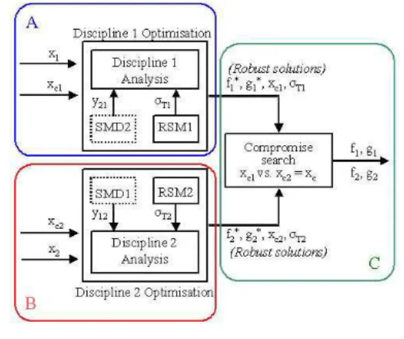
Concurrent Engineering [20] - was developed under the following specifications: reduced design time, implemen-tation ease and guarantee of satisfactory and feasible solutions. It is based on a robust design approach: finding solutions that are robust with respect to changes in variable values due to discipline interactions. The MORDACE approach allows to independently perform the different discipline optimizations, as shown in Fig. 4.
Each discipline aims at finding optimal solution with respect to its own design variables thank to a Multi-Objective Genetic Algorithm (MOGA) in order to obtain for each discipline the Pareto frontier as the set of best solution design. When independent optimization processes finish, the designer has to find a compromise on common variable values (step C in Fig. 4). Changes in common variable values due to compromise could worsen performance levels. So in addition to design objectivesfi, disciplines aim to minimize the effect of variation
in values of common variables. As disciplines simultaneously minimize objective functions fi and sensitive
function, they are always multi-objectives. Among available designs, the procedure chooses Pareto designs plus all individuals that dominate the original one with regard to different disciplines. Then, it defines all possible couples made up of solutions proposed by discipline 1 and 2, respectively. At this stage, the calculation of a distance parameter allows efficient solutions to be sorted out from the very large set of all possible couples. Thus, a limited number of couples are automatically chosen. Those solutions show small difference between discipline 1 and 2 common variable values and they are robust with regard to changes in those values. Then, performances and coupling functions of the compromise designs defined by the new vectors of variables have to be verified.
Within the MORDACE method the designer needs to use a compromise method limited by the number of evaluation of potential solutions the designer allows. The methods described hereafter introduce a loop between system level and sub-system level in order to guide the discipline optimization thank to a view of the global problem.
4.2 E-MMGA
These method relies on a decomposition of the optimization at the disciplinary level. A first proposal was given in [22], but do not take into account the coupling functions and was limited to hierarchical system.
Each multiobjective GA at the subproblems operates on its own population of (xsh, xj). The population
size, P , for each subproblem is kept the same. In addition, E-MMGA maintains two populations external to the subproblems: the grand population and the grand pool that both are populations of complete design variable vector: (xsh, x1, ..., xJ). The grand population is an estimate of the solution set to the overall optimization
problem. The grand pool is an archive of the union of solutions generated by the subproblems. The size of the grand population is the same as the subproblem population size,P . The size of the grand pool is J times the size of the subsystem’s population.
Figure 5: E-MMGA method The population of the grand population are used as the
ini-tial population for each subproblem. Since the subproblem mul-tiobjective GAs operates on its own variables(xsh, xj), only the
chromosomes corresponding to xsh andxj are used in thejth
subproblem. After each run of subproblem multiobjective GA there will beJ populations having P individuals each. As each of the J populations contains only the chromosomes of only (xsh, xj), j = 1, ..., J, they are completed using the rest of the
chromosome sequence(x1, ..., xj−1, xj+1, ..., xJ) from the grand
pool. After the chromosomes in all J populations are reconsti-tuted to form the complete design variable vector, they are added to the grand pool. Then based on an entropy index that preserve the diversification of the solutions set,P individuals are chosen within the grand pool and replace the P individuals from the grand population.
An important drawback is that the size of the grand pool in-creases very quickly with the number of disciplines and individu-als. A variant has been proposed in [23], in each subsystem only one solution is selected on the Pareto frontier and its objectives and constraints values will be used to assign a fitness value for the
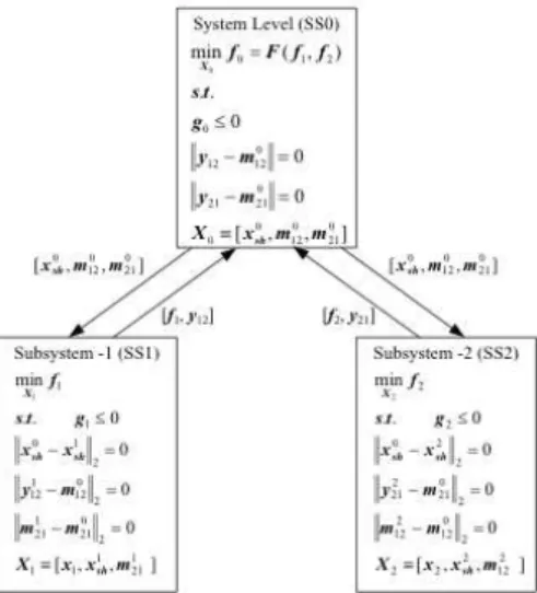
system level individual. The so-called best solution for each disciplines is chosen by an algorithm thank to the designer or decision maker preferences. The coupling functions are taken into account thanks to supplementary constraints -added both at system and subsystem levels- and auxiliary variables (see Fig. 5). Note that the shared variables can be treated as parameters in the subsystems and its reduces the dimensionality of the subsystem level optimization problems. In this last case, the coupling variable values are not passed to the system level.
4.3 COSMOS
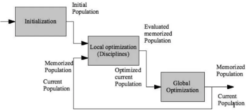
COSMOSmethodologies ([25]) have been developed in order to facilitate and increase performances of de-sign and optimization of complex systems in the context of extended enterprises. This methodology intends to reproduce a process adapted to the structure in which designers work. The main goal of such methodologies is to provide an ideal enterprise work process by taking into account its organization, its resources and its tools. The final aim is to allow ideal design processes in companies’ usual structures, such as extended enterprises. The philosophy which has led COSMOS elaboration consist in adapting the optimization algorithm to the companies’ uses and not to the other way round.
Two variants (COSMOS G and COSMOS L ([26])) have been proposed and the fundamental difference be-tween them resides in a different treatment of coupling design variables. During the initialization the supervisor creates a population of common design variablesxCand each disciplinei also creates a population of disciplinary
variablesxi: the size of all population is the same,popsize. In order to get a fully determined population, the
supervisor sends the vector of coupling design variablesxC to each discipline. Each disciplinei builds a
disci-plinary population{xC, xi} for which it can evaluate objective and constraint functions. An initial population can
be created by the aggregation of common and disciplinary design variables and saved in (P opmemorized).
Optimization at sub-system level: In COSMOS G, the supervisor provides a set of common design variablesxC
to the disciplines. Each disciplinei optimizes the design variables of a population of individuals {xC[j], xi[j]}
where j ∈ [1..popsize]. The vector xC is fixed in order to keep the disciplinary population coherent with
the other disciplinary populations. At the end of the disciplinary optimizations, each discipline sends a vec-tor of disciplinary design variables optimized xi,opt to the supervisor. Since the vector of common design
variables has not been modified in the discipline, a global population can be built and is naturally coherent: P opcurrent= {x1,opt, . . . , xN OD,opt, xC}.
In COSMOS L, each discipline optimizes the design variables of its population of individuals{xC[j], xi[j]}
(where j ∈ [1..popsizei] - P opSizei is the size of the discipline i population), but vector xC is not fixed
anymore. At the end of the disciplinary optimizations, each discipline population is composed as follows: P opdisci,opt = {xi,opt, xCi,opt} where xCi,opt is the vector of common design variables optimized in the
dis-ciplinei. An important remark is that the size of the population in each discipline can be different.
Optimization at system level: In COSMOS G, at the supervisor level, the goal is to propose new and better common design variables (in order to improve the population). So, the current population (P opcurrent) is
assem-bled with the memorized population (P opmemorized) in order to provide a double-sized population (P opdouble).
This population is ranked by the Fonseca and Fleming’s criterion (notion of Pareto domination) according to all the objective functions of the problem. The best individuals are selected to build a normal-sized population (P opcurrent). This population will be send to the disciplines. In parallel, cross-over and mutations are made on
the common design variables of the population. This new population is saved in memory (P opmemorized). It will
be evaluated once by the disciplines in order to determine its objective and constraint functions.
Figure 6: General description of COSMOS family algorithm In COSMOS L, the vectors of
cou-pling design variables provided by the disciplines are inherently different, since each discipline optimizes not only disci-plinary design variables but also common ones. Disciplinary populations provided by discipline i are composed as follows P opdisc−i,opt= {xi,opt, xC−i,opt}. In
or-der to build a global and coherent popu-lation, N1 individuals are randomly
cho-sen in each disciplinary population. Si-multaneously, a table ofN2positive
coeffi-cients is randomly created.N1andN2are
chosen by the designer so thatN1.N2 =
P opSize, where P opSize is the size of the
design variables obtained by disciplinary optimizations into the global population and by creating compromises on common design variables thanks to a barycentre-based construction. Such a procedure enables each discipline to work with a specific size of population.
Coupling functions treatment: If coupling functions between sub-level disciplines have to be considered, an approximation of their values are provided by the system level. The difference between the real, but inaccessible, value and the approximated value decreases during the optimization process because variations decrease in the same time. One can also note that the optimization time can be different from one discipline to the others. At the end of the optimization process, each discipline sends to the supervisor a table which contains the values of disciplinary design variables and the associate objective, constraint and coupling functions. At the supervisor level, the values of coupling functionyj,icomputed by disciplinej are sent to discipline i. These values will be
used by disciplinei at the disciplinary level in order to process the optimization of the sub-system i. When the optimization process evolves in disciplinej, the values of yj,ialso evolve and then, the values used by discipline
i become approximations. Nevertheless, we have noticed on the experimentation we have carried out that the difference between the values ofyj,iand their related approximations decrease during the optimization process
because of the convergence of the population. Anyway, the difference is reset to zero when supervisor provides exact values of coupling functions from disciplinej to discipline i.
4.4 Evaluation - Conclusion
These three methods have been tested on several examples and E-MMGA et COSMOS have obtained similar Pareto frontier for the well-known Golinski’s speed reducer problem. One criticism made on these methods combining GA and MDO is their computational cost (thanks to the evaluations within the GA). Our opinion is that it is important to obtain a representation of the whole solution space (and not only a single point) and if an optimization process allows to improve the final system with an acceptable ROI, it is acceptable.
5 Conclusion - Perspectives
In this paper, a brief review of MDO methodologies has been presented. The classic mono- and bi-level ones have been described in a first part and the different methods’ formulation are shown on an example. Based on our own tests and several bibliographical papers, the comparison between the methodologies is not easy and some criteria are subjective. Some researches have to be done in order to explain with more details the different criteria used in the comparative tests and to propose new ones. It seems also important to identify for each methods the factors that have some influences on the results. Besides it would help to identify the best process and the most adapted approach for a given typology of MDO problems.
The second part presents a different group of methods: approaches combining Evolutionnary Algorithms and Collaborative Optimization. Collaborative optimization provides the structure for the optimization process and allows the hierarchical decomposition of the problem into multiple levels with separate sets of design variables. The MOGA’s strength of obtaining a set of optimal solutions (Pareto frontier) is exploited in each discipline. These methods are promising as they (i) allow the designer to obtain a global view of design space, (ii) can be easily used in an industrial context - each team can used its own tools, analysis algorithmes, . . . Some improvements can be done and more tests on industrial problems have to be performed. Moreover it would be of great interests to define a data base of tests with different complexity (number of coupling and common variables and different number of disciplines, including different type of analysis and evaluation). This DB could be used by every researchers as tests for their new MDO developments.
References
[1] MDO-Technical-Committee Current state of the art in multidisciplinary design optimization AIAA
Techre-port, 1991
[2] Giesing J. P. and Barthelemy J. M. A summary of industry MDO applications and needs In 7-th
AIAA/USAF/NASA/ISSMO, 1998
[3] Marler R.T. and Arora J.S. Survey of multi-objective optimi-zation methods for engineering Struct.
Multi-disciplinary Optimization, 2004, Vol. 26, 369-395.
opti-mization for single-level formulations DETC’05 - ASME Design Engineering Technical Conferences, 2005, Long Beach, USA.
[5] Wagner T. A general decomposition methodology for optimal system PhD Thesis, University of Michigan, 1993
[6] Choudhary R., Malkawi A. and Papalambros P. Analytic target cascading in simulation-based building de-sign Automation in construction, 2005, Vol.14, 551-568
[7] Cramer E. J., Dennis J. E., Frank P. D., Lewis R. M. and Shubin, G. R. Problem Formulation for Multidisci-plinary Optimization SIAM Journal of Optimization, 1994, Vol. 4, 754-776
[8] Balling R. J. and Sobieszczanski-Sobieski J. Optimization of Coupled Systems : A critical Overview of Approaches In AIAA Journal, 1996, Vol. 34, 6-17
[9] Kodiyalam S. Evaluation of Methods for Multidisciplinary Design Optimization (M.D.O.), Phase 1.
CR-1998-20871- NASA, 1998, Vol. 6
[10] Tappeta R. V. and Renaud J. Multiobjective collaborative optimization Trans. of ASME, Journal of
Mechan-ical Design, 1997,Vol. 119, 403-411.
[11] Alexandrov N. M. and Lewis R. M. Comparative Properties of Collaborative Optimization and Other Ap-proaches to MDO ICASE-99-24; NAS 1.26209354; NASA CR-1999-209354, 1999
[12] Hulme K. F. and Bloebaum C. L. A Simulation-based Comparison of Multidisciplinary Design Optimization Solution Strategies using CASCADE Structural and Multidisciplinary Optimization, 2000, Vol. 19, N. 1, 17-35,
[13] Behdinan K., Perez R. E. and Liu H. T. Multidisciplinary design optimization of aerospace systems
Pro-ceedings of the 2nd International Design Conference CDEN, 2005
[14] Dennis J.E., Arroyo S.F., Cramer E.J. and Frank P.D. Problem formulations for systems of systems IEEE
International Conference on Systems, Man and Cybernetics, 2005, Vol.1, 64-71.
[15] Braun R., Cage P., Kroo I. and Sobieski I., Implementation and performance issues in collaborative opti-mization 6th AIAA/NASA/ISSMO Symposium on Multidisciplinary Analysis and Optiopti-mization, 1996, Vol. 1, 295-305
[16] Wujek B., Renaud J. and Batill S., A Concurrent Engineering Approach for Multidisciplinary Design in a Distributed Computing Environment Multidisciplinary Design Optimization: State of the Art , N. Alexandrov
and M. Y. Hussaini, editors, SIAM, 1997.
[17] Sobieszczanski-Sobieski J., Agte J. and Sandusky Jr., R. Bi-level integrated system synthesis (BLISS)
NASA/TM-1998-2087151998
[18] Allison J. T., Kokkalaras M. and Papalambros, P. Y., On the use of analytical target cascading and collab-orative optimization for complex system design 6th World Conference on Structural and Multidisciplinary
Optimization2005
[19] McAllister C. D., Simpson T. W. and Lewis K. and Messac A. Robust multiobjective optimization through collaborative optimization and linear programming 10th AIAA/ISSMO Multidisciplinary Analysis and
Opti-mization Conference, 2004
[20] Giassi A., Bennis F. and Maisonneuve J.-J. Multi-disciplinary design optimization and robust design ap-proaches applied to concurrent design Structural and Multidisciplinary Optimization 2004
[21] Gu X., Renaud J. E., Ashe L. M., Batill S. M., Budhiraja A. S. and Krajewski L. J. Decision-Based Collab-orative Optimization, In Journal of Mechanical Design, ASME, 2002, 124, 1-13
[22] Gunawan S., Farhang-Mehr A. and Azarm S. Multi-level Multi-Objective Genetic Algorithm Using En-tropy to Preserve Diversity In Proceedings of the Second International Conference on Evolutionary
Multi-Criterion Optimization, 2003, 148-161
[23] Aute V. and Azarm S. A Genetic Algorithms Based Approach for Multidisciplinary Multiobjective Collab-orative Optimization 11th AIAA/ISSMO Multidisciplinary Analysis and Optimization Conference 2006 [24] Kodiyalam S. and Sobieszczanski-Sobieski J. Multidisciplinary design optimization: some formal methods,
framework requirements, and application to vehicle design In Int. J. Vehicle Design, 2001, 3-22
[25] Rabeau S., D´epinc´e P. and Bennis F. COSMOS: Collaborative Optimization Strategy for Multi-Objective Systems In International Symposium series on Tools and Methods of Competitive Engineering, 2006. [26] Comparison of global and local treatment for coupling variables into multidisciplinary problems Rabeau
S., D´epinc´e Ph., Bennis F. and Janiaut R. 11th AIAA/ISSMO Multidisciplinary Analysis and Optimization