HAL Id: hal-01302411
https://hal.archives-ouvertes.fr/hal-01302411
Submitted on 14 Apr 2016
HAL is a multi-disciplinary open access
archive for the deposit and dissemination of
sci-entific research documents, whether they are
pub-lished or not. The documents may come from
teaching and research institutions in France or
abroad, or from public or private research centers.
L’archive ouverte pluridisciplinaire HAL, est
destinée au dépôt et à la diffusion de documents
scientifiques de niveau recherche, publiés ou non,
émanant des établissements d’enseignement et de
recherche français ou étrangers, des laboratoires
publics ou privés.
An extension of the ICA model using latent variables
Selwa Rafi, Marc Castella, Wojciech Pieczynski
To cite this version:
Selwa Rafi, Marc Castella, Wojciech Pieczynski. An extension of the ICA model using latent variables.
ICASSP 2011 : 36th International Conference on Acoustics, Speech and Signal Processing, May 2011,
Prague, Czech Republic. pp.3712 - 3715, �10.1109/ICASSP.2011.5947157�. �hal-01302411�
AN EXTENSION OF THE ICA MODEL USING LATENT VARIABLES
Selwa Rafi, Marc Castella, and Wojciech Pieczynski
Institut Telecom; Telecom SudParis
D´epartement CITI; UMR-CNRS 5157
9 rue Charles Fourier, 91011 Evry Cedex, France
ABSTRACTThe Independent Component Analysis (ICA) model is ex-tended to the case where the components are not necessarily independent: depending on the value a hidden latent process at the same time, the unknown components of the linear mix-ture are assumed either mutually independent or dependent. We propose for this model a separation method which com-bines: (i) a classical ICA separation performed using the set of samples whose components are conditionally independent, and (ii) a method for estimation of the latent process. The latter task is performed by Iterative Conditional Estimation (ICE). It is an estimation technique in the case of incomplete data, which is particularly appealing because it requires only weak conditions. Finally, simulations validate our method and show that the separation quality is improved for sources generated according to our model.
Index Terms— Independent Component Analysis (ICA),
blind source separation, Iterative Conditional Estimation (ICE)
1. INTRODUCTION
For the last decades, Blind Source Separation (BSS) has been an active research problem: this popularity comes from the wide panel of potential applications such as audio processing, telecommunications, biology,. . . In the case of a linear multi-input/multi-output instantaneous system, BSS corresponds to Independent Component Analysis (ICA), which is now a well recognized concept [6]. Contrary to other frameworks where techniques take advantage of a strong information on the di-versity, for instance through the knowledge of the array mani-fold in antenna array processing, the core assumption in ICA is much milder and reduces to the statistical mutual indepen-dence between the inputs. However, the latter assumption is not mandatory in BSS. For instance, in the case of static mix-tures, sources can be separated if they are only decorrelated, provided that their nonstationarity or their color can be ex-ploited. Other properties such as the fact that sources belong to a finite alphabet can alternatively be utilized [5, 11] and do not require statistical independence.
We investigate a particular model which combines an ICA model with a probabilistic model on the sources, mak-ing them either dependent or independent at different time
instants. Our method exploits the ”independent part” of the source components. Although it is possible to refine our model by introducing a temporal dependence, it assumes nei-ther nonstationarity nor color of the sources. To our knowl-edge, only few references have tackled this issue in such a context [2, 4, 8], although the interest in dependent sources has been witnessed by some works in applied domains [1, 9]. Finally we would like to outline the difference between our work and [1]: the latter assumes a conditional independence of the sources, whereas, depending on a hidden process, we assume either conditional independence or dependence.
In the whole paper, N (0, I) stands for a zero mean Gaus-sian law, with identity covariance matrix. L(λ) denotes the scalar Laplace distribution with parameter λ. We will use ∼ to indicate the distribution followed by a random variable and r | X; θ will refer to the law of r conditionally on X under parameter values θ.
2. EXTENDED ICA MODEL 2.1. Linear mixture
We consider a set of T samples of vector observations. At each time instant t ∈ {1, . . . , T } the observed vector is denoted by x(t) , (x1(t), . . . , xN(t))
T
. We assume that these observations result from a linear mixture of N un-known and unobserved source signals. In other words, there exists a matrix A ∈ RN ×N and a vector valued process
s(t) , (s1(t), . . . , sN(t))
T
such that:
x(t) = As(t), ∀t ∈ {1, . . . , T }. (1)
Let X , (x(1), . . . , x(T )) be the N × T matrix with all ob-servations and S , (s(1), . . . , s(T )) be the Q×T matrix with all sources. The matrix A is unknown and the objective con-sists in recovering S from X only: this is the so-called blind
source separation problem. We will assume here that A is
in-vertible and the problem thus resumes to the estimation of A or its inverse B. A solution has been developed for long and is known as ICA [6]. It generally requires two assumptions: the source components should be non Gaussian –except pos-sibly one of them– and they should be statistically mutually independent. With these assumptions, it is known that one
can estimate a matrix B ∈ RN ×N such that y(t) = Bx(t)
restores the sources up to some ambiguities, namely ordering and scaling factor. In the following, B denotes an inverse of A up to these ambiguities.
2.2. Latent variables
In this work, we extend ICA methods and relax in a certain way the independence assumption. The basic idea consists in introducing a hidden process r(t) such that, depending on the particular value of r(t) at instant t, the independence as-sumption is relaxed at time t. Let r , (r(1), . . . , r(T )). We assume more precisely:
A1. Conditionally on r, the components s(1), . . . , s(T ) of S at different times are independent.
A2. The hidden process r(t) has values in {0, 1} and, con-ditionally on r(t):
(i) when r(t) = 0, the components of s(t) are mutu-ally independent and non Gaussian, except possi-bly one of them;
(ii) when r(t) = 1, the components of s(t) are depen-dent.
In a BSS context, one can see that, if r were known, one could easily apply ICA techniques by discarding the time in-stants where the sources are dependent. To be more precise, let I0 , {t ∈ {1, . . . , T } | r(t) = 0} be the set of time
in-stants where the components of s(t) are independent. Then the subset X0 , (x(t))t∈I0 of the whole set X of the
ob-servations satisfies the assumptions usually required by ICA techniques. The main idea in our article consists in perform-ing alternatively and iteratively an estimation of B (corre-sponding to A−1) and of the hidden data r.
2.3. Typical sources separated by our method
The sources that we consider satisfy Assumptions A1 and A2. To illusrate Assumption A2, let us give an example with N = 2 sources which will be considered in simulations. Let
u , √1 2 µ s1(t) + s2(t) s1(t) − s2(t) ¶ . (2)
When r(t) = 1, that is, when the sources are dependent, we will consider in A2-(ii) that P(s(t) | r(t) = 1) is such that u ∼ L(λ) × N (0, 1) with λ = 2. The components of u are hence independent and follow respectively a Laplace and Gaussian law. It is not required to specify further A2-(i), but for illustration, we will consider that P(s(t) | r(t) = 0) is such that the components of s(t) are independent and uni-formly distributed. Such a distribution density is illustrated by simulated values in Figure 1(a). A density of some mixed observations is also shown in Figure 1(b). Considering X0
only amounts to removing the cloud set of dependent points on the distributions of Figure 1.
(a) (b)
Fig. 1. (a) Density plot of the sources s: independent components with probability P(r(t) = 0) = p = 0.7. (b) Observations x = As with: A = (0.3 0.8
0.1 0.1)
3. PARAMETER ESTIMATION FROM INCOMPLETE DATA
3.1. Context
Let us denote by θ the set of parameters to be estimated from the data: here, θ consists of the matrix B and of the param-eters which give the distribution of r. Let us call (r, X) the set of complete data, whereas X alone is the set of incomplete data: since r is a hidden process, the model described in Sec-tion 2 corresponds to the situaSec-tion where only incomplete data is available for estimation of the searched parameters θ. Note that the adjective blind is used to emphasize that S is unavail-able, whereas incomplete emphasizes that r is unavailable. 3.2. Iterative conditional estimation
Iterative conditional estimation (ICE) is an iterative estima-tion method that applies in the context of incomplete data and that has been proposed in the problem of image segmenta-tion [10, 12]. Starting from an initial guess of the parameters, the method consists in finding iteratively a sequence of esti-mates of θ, where each estimate is based on the previous one. More precisely, if ˆθ[0]is the first guess, the sequence of ICE
estimates is defined by: ˆ
θ[q]= E{ˆθ(r, X) | X; ˆθ[q−1]} (3) where E{. | X; ˆθ[q−1]} denotes the expectation
condition-ally on X and with parameter values ˆθ[q−1]. In practice, the
previous conditional expectation can be replaced by a sample mean, that is (3) can be replaced by:
ˆ θ[p]= 1 K K X k=1 ˆ θ(r(k), X) (4)
where K ∈ N∗ is fixed and each r(k)is drawn according to
the a posteriori law r|X; ˆθ[q−1]. The prerequisites in order to
• there exist an estimator from complete data ˆθ(r, X), • one is able either to calculate E{. | X; ˆθ[q−1]} or to
draw random variables according to r|X; ˆθ[q−1].
These two conditions are very weak, which is the reason of our interest in ICE. In fact concerning the former one, there would be no hope to perform incomplete data estimation if no complete data estimator exists, whereas the second require-ment consists only in being able to simulate random values according to the a posteriori law.
4. ASSUMED DISTRIBUTION FOR (r, S) In this Section, we describe the assumptions on which our method relies. These assumptions on the probabilistic model describing the unknown data (r, S) do not exactly correspond to the source model given in section 2.3, although they are used in the ICE method.
As specified above, the observed data is given by a linear transformation of S according to Equation (1). Combining a statistical model on (r, S) with an ICA model on (S, X) yields a genuine model. In a more classical context, we would indeed have:
• either the ICA model of Equation (1) with an
indepen-dence assumptions on s(t), which is much simpler than assumption A2.
• or a probabilistic model written on (r, X) and no
par-ticular relation such as (1).
For simplicity, we assume in the following N = 2, which also corresponds to our simulation settings. However, the method is theoretically valid for any value of N .
4.1. Specification of assumption A2
In the estimation algorithm, we assume, similarly to A1, that the probability law P(r, S) factorizes:
P(r, S) = P(r)
T
Y
t=1
P(s(t) | r(t))
where P(s(t) | r(t) = 1) is such that the components ui, i =
1, 2 of the vector u in (2) both follow ui ∼12L(λ)+12N (0, 1)
with λ = 2. In the other words, when r(t) = 1, each com-ponent of u is modelized as a mixture of the probability den-sities of a Gaussian and a Laplace law. This distribution is a symmetrical analog to the one in Section 2.3: although it is not the real distribution of the sources, such a symmetry is necessary in our method because ICA methods generally leave permutation ambiguities. Finally, when r(t) = 0, we consider P(s(t) | r(t) = 0) ∼ N (0, I). Again, because of A2-(i), this does not correspond to the true distribution but to the model used by the ICE method.
4.2. Hidden process r model
In the simplest version of our method, no assumption is made on r. This amounts to modeling r as an i.i.d. Bernoulli pro-cess, that is P(r) =QTt=1P(r(t)) with P(r(t) = 0) = p and P(r(t) = 1) = 1 − p. The parameters p can be estimated by the ICE method.
An extension consists in modeling r as a stationary Markov chain, in which case the temporal dependence of r is taken into account. In this case, the probability distribu-tion of r is given by: P(r) = P(r(1))Qt=Tt=2P(r(t) | r(t − 1)) where P(r(t) | r(t − 1)) is given by a transition matrix inde-pendent of t. The main advantage of considering a Markov model is that P(r | X; θ) can be calculated by an efficient forward-backward algorithm [7], making ICE method appli-cable [10].
4.3. Data parameters
In our simulations, the process r has been generated either i.i.d. (Section 5.2.1) with P(r(t) = 0) = p, P(r(t) = 1) = 1 − p or as a Markov chain (Section 5.2.2). The sources are generated following the description in Section 2.3 and mixed according to (1). The mixing matrix A is drawn randomly.
5. SIMULATIONS 5.1. Summary of the algorithm
Our proposed method combines ICA and ICE. The com-plete data estimator ˆθ(r, X) in Section 3.2 is provided by
one of the existing ICA separation methods. We denote it by ICA in the summary of our algorithm which follows:
Initialize the parameters ˆθ[0]= ( ˆB[0], ˆp[0]).
For q = 1, 2, . . . , qmax, repeat:
• calculate P(r | X; ˆθ[q]) and draw ˆr[q]according to this
distribution ,
• set: ˆI0[q]= {t | ˆr[q](t) = 0} and ˆX[q]
0 = (x(t))t∈ˆI[q]0
• B[q+1]ˆ = ICA( ˆX[q] 0 )
• update the parameters of the process r.
In the simplest case where r is i.i.d., the last step above consists in updating the estimated value of p according to ˆ
p[q+1] = 1
T
PT
t=1P(r(t) = 0 | x(t), ˆθ[q]). Finally, note that
the above method estimates p according to (3), whereas B is estimated according to (4) with K = 1.
5.2. Results
We compare now the separation quality using only a classical ICA method or the same ICA method combined with ICE as proposed. In the simulations, the chosen ICA algorithm is the JADE algorithm for real data [3]. The number of ICE iterations has been fixed empirically to qmax = 20. We show
here the values of the mean square error (MSE) on the two retrieved sources. All the given results have been obtained by an average over a set of 1000 Monte-Carlo realizations.
5.2.1. i.i.d. latent variable
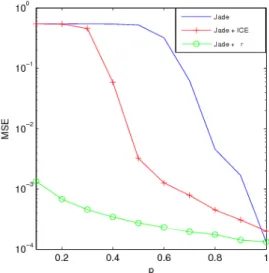
We have first tried our method with r i.i.d. Figure 2 shows the MSE for different values of p and for different methods: JADE applied on X, our method combining JADE and ICE (JADE + ICE) and JADE applied on X0 (JADE + r). The
latter case is an ideal situation which would only apply when complete data is available. We clearly see that our method succeeded in separating sources for values of p greater than 0.4. The quality improvement of our method in comparison to JADE is clearly observed for p between 0.4 and 0.9 ap-proximately. We also studied the influence of the number of samples. The results are presented in Table 5.2.1, where we have considered the value p = 0.5. We can see from Table 5.2.1 that our method is advantageous for all samples sizes.
Fig. 2. Average MSE on the sources depending on p and for
T = 5000 samples.
T JADE JADE + r JADE + ICE 1000 3.7 10−1 1.4 10−3 3.8 10−2
2000 4.4 10−1 0.6 10−3 1.4 10−2
5000 5.1 10−1 0.2 10−3 2.9 10−2
10000 5.4 10−1 0.1 10−3 1.3 10−2
Table 1. Average MSE for different sample sizes and p = 0.5.
5.2.2. Markov latent variable
We have tested our method in the case where the process r of the simulated data is a stationary Markov chain with transition matrix (0.9 0.1
0.1 0.9). We have compared the MSE values obtained
with our method ”JADE + ICE” based on a Markov model for r and ”JADE + ICE” based on an i.i.d. model for r. The re-sults in Table 5.2.2 show that taking into account the Markov dependence of r significantly improves the quality result.
T Markov model i.i.d. model 1000 0.9 10−1 1.7 10−1
5000 2.1 10−3 3.3 10−3
Table 2. MSE for the i.i.d. model and the Markov model. 6. REFERENCES
[1] S. Akaho. Conditionally independent component anal-ysis for supervised feature extraction. Neurocomputing, 49:139–150, December 2002.
[2] J.-F. Cardoso. Multidimensional independent compo-nent analysis. In Proc. ICASSP ’98. Seattle, 1998. [3] J.-F. Cardoso and A. Souloumiac. Blind
beamform-ing for non gaussian signals. IEE-Proceeding-F,
140(6):362–370, December 1993.
[4] M. Castella and P. Comon. Blind separation of instan-taneous mixtures of dependent sources. In Proc. of
ICA’07, volume 4666 of LNCS, pages 9–16, London,
UK, September 2007.
[5] P. Comon. Contrasts, independent component analysis, and blind deconvolution. Int. Journal Adapt. Control
Sig. Proc., 18(3):225–243, Apr. 2004.
[6] P. Comon and C. Jutten, editors. Handbook of Blind
Source Separation, Independent Component Analysis and Applications. Academic Press, 2010.
[7] P. A. Devijver. Baum’s forward-backward algorithm re-visited. Pattern Recognition Letters, 3:369–373, 1985. [8] A. Hyv¨arinen and S. Shimizu. A quasi-stochastic
gradi-ent algorithm for variance-dependgradi-ent compongradi-ent analy-sis. In Proc. International Conference on Artificial
Neu-ral Networks (ICANN2006), pages 211–220, Athens,
Greece, 2006.
[9] F. Kohl, G. W¨ubbeler, D. Kolossa, C. Elster, M. B¨ar, and R. Orglmeister. Non-independent BSS: A model for evoked MEG signals with controllable dependencies. In
Proc. of ICA’09, volume 5441 of LNCS, pages 443–450,
Paraty-RJ, Brazil, March 2009.
[10] P. Lanchantin, J. Lapuyade-Lahorgue, and W. Pieczyn-ski. Unsupervised segmentation of randomly switching data hidden with non-gaussian correlated noise. Signal
Processing, 91:163–175, February 2011.
[11] T.-H. Li. Finite-alphabet information and multivariate blind deconvolution and identification of linear systems.
IEEE-IT, 49(1):330–337, January 2003.
[12] W. Pieczynski. Statistical image segmentation. Machine