National Bank of Belgium
Limited liability company
RLP Brussels – Company number : 0203.201.340 Registered office : boulevard de Berlaimont 14 BE - 1000 Brussels
www.nbb.be
The political economic of fi nancing climate policy :
evidence from the solar PV subsidy programs
by Olivier De Groote, Axel Gautier and Frank Verboven
Working Paper Research
October 2020 N° 389
Editor
Pierre Wunsch, Governor of the National Bank of Belgium
Editoral
On October 22-23, 2020 the National Bank of Belgium hosted a Conference on “Climate Change: Economic Impact and Challenges for Central Banks and the Financial System”. Papers presented at this conference are made available to a broader audience in the NBB Working Paper Series (www.nbb.be). This version is preliminary and can be revised.
Statement of purpose:
The purpose of these working papers is to promote the circulation of research results (Research Series) and analytical studies (Documents Series) made within the National Bank of Belgium or presented by external economists in seminars, conferences and conventions organized by the Bank. The aim is therefore to provide a platform for discussion. The opinions expressed are strictly those of the authors and do not necessarily reflect the views of the National Bank of Belgium.
Orders
The Working Papers are available on the website of the Bank: http://www.nbb.be.
© National Bank of Belgium, Brussels All rights reserved.
Reproduction for educational and non-commercial purposes is permitted provided that the source is acknowledged. ISSN: 1375-680X (print)
The political economy of financing climate policy –
evidence from the solar PV subsidy programs
Olivier De Groote, Axel Gautier and Frank Verboven
* October 2020 Abstract To combat climate change, governments are taking an increasing number of technology-specific measures to support green technologies. In this paper, we look at the very generous subsidy policies to solar PVs in the three regions of Belgium to ask the question of how voters responded to these programs. We provide evidence that voters did not reward the incumbent government that was responsible for the program, as predicted by the ‘buying-votes’ hypothesis. Instead, we find that voters punish the incumbent government because of the increasing awareness of the high financing costs. These did not only affect the non-adopting electricity consumers who did not benefit from the programs, but also the adopting prosumers, who saw unannounced new costs such as the introduction of prosumer fees to get access to the grid. * Olivier De Groote, Toulouse School of Economics, University of Toulouse Capitole, Toulouse, France ([email protected]). Axel Gautier, HEC Liège, University of Liège ([email protected]). Frank Verboven, Department of Economics, KU Leuven ([email protected]). The financial support of the National Bank of Belgium is gratefully acknowledged.Contents 1 Introduction ... 4 2 Subsidy programs to promote residential PV installations ... 7 2.1 Types of subsidy programs ... 7 2.1.1 Rebates on the investment costs ... 8 2.1.2 Green certificates (GCs) ... 8 2.1.3 Net metering ... 9 2.2 Evolution of the magnitude of the programs ... 10 2.2.1 Computing the net present value components ... 10 2.2.2 Evolution of the benefits of the PV subsidy programs ... 11 3 The impact of the subsidy programs on PV adoption ... 13 3.1 The determinants of PV adoption: a descriptive approach ... 14 3.1.1 Model and data ... 15 3.1.2 Empirical results ... 16 3.2 The dynamics of PV adoption ... 19 3.2.1 Dynamic model and data ... 20 3.2.2 Empirical results ... 21 4 Financing issues of the policies and the political debate ... 23 4.1 Financing issues ... 23 4.1.1 Investment support ... 23 4.1.2 GC system ... 23 4.1.3 Net metering ... 24 4.2 Evolution of electricity prices ... 25 4.3 Political debate ... 26 4.4 Political responsibility ... 27 5 Voters’ responses to the subsidy programs ... 27 5.1 Hypotheses ... 28 5.2 Model and data ... 28 5.3 Empirical results ... 29 6 Conclusion ... 33 1 Appendix: sources of policy and net present value ... 35 1.1 Investment costs ... 35 1.2 Government policies ... 35 1.3 Electricity prices ... 36 1.4 Assumptions net present value ... 36 2 Appendix: further details of the dynamic model ... 37
3 Appendix: further details on the voting model ... 39 4 Appendix: additional results on votes ... 40
1 Introduction
There is now a broad consensus among scientists that the massive increase in CO2 emissions has been responsible for the climate change observed over the past decades. There is also a growing awareness that drastic policies are required to reduce the CO2 emissions and prevent a further acceleration of global warming in the future.
However, there is much less consensus on the type of policies that are required to reduce CO2 emissions. Economists often favour Pigouvian taxes on CO2 emissions to correct for the externalities.1 But such taxes may not be politically feasible for a variety of reasons: distributional concerns, industry pressure, aversion to taxes, lack of coordination, or fiscal competition between countries (see e.g. Fowlie, 2019). As a result, politicians have often favored a variety of subsidy programs to promote specific renewable energy sources (RES), such as solar, wind or biofuel, and more generally to support the adoption of green technologies. Governments have used a wide range of instruments, including tax incentives, investment subsidies and production subsidies. In this paper, we aim to better understand the political economy that lies behind technology-specific subsidies. We exploit the unique setting of the generous subsidy programs to solar photovoltaic (PV) systems in Belgium. Each of the country’s three regions adopted similar policies, consisting of a combination of rebates of part of the investment costs and subsidies on green electricity production. Because policies led to massive adoption, two of the three regions also needed to cope with comparable financing problems, and it led to continuous political debate. The main policies were designed during the period 2004-2009 by the regional governments, which at that time were center or center-left coalitions in the three regions. Because the regions differed in their timing and magnitude of the programs, and because they had separate political responsibilities towards their voters, this provides an interesting setting to understand how voters responded to these programs. In particular, we first consider their decision to adopt or not the solar technology. Next, we see if and how, technology adopters and non-adopters modified their vote to eventually reward or punish the politicians who designed these programs.
Our analysis consists of different parts. First, we describe the various types of subsidy programs that have been introduced. An important feature of our setting is that the programs quickly shifted away from rebates to future production subsidies under the form of Green Certificates (GCs) and net-metering.2 Under net metering, the energy produced by the solar panels is valued at the retail price, including all taxes and surcharges. With a mechanical meter (the most common metering technology in Belgium in the absence of smart meters), net metering is simply implemented by having the meter running backwards when the solar production exceeds the house’s consumption. This shift to production subsidies, granted for long periods, implies that the financing of the programs is postponed to the future and current technology adopters are financed by future energy consumers. Moreover, it requires a larger budget, because households are more responsive to upfront subsidies i.e. they discount these future benefits too heavily (De Groote and Verboven, 2019). Second, we show how
1 See, for example, the Economists’ Statement on Carbon Dividends
(https://clcouncil.org/economists-statement), written in January 2019, and signed by 27 Nobel laureates and 15 former chairs of the US Council of Economic Advisers.
2 One reason for abandoning the investment subsidies may have been the fact that EU fiscal rules impose
governments to fully cover the costs of environmental investment subsidies, even if they imply productive future benefits (see De Grauwe, 2018).
the programs led to massive adoption of solar PVs. This highlights again the central role of the generous GCs. Third, given the magnitude and success of the GC system to promote adoption, the financing of the program became critical, leading to intense political debate and discussions. These financing issues raised important redistributional concerns. A central question was who should pay for the generous subsidies: technology adopters or non adopters; and current or future consumers? The financing of these costs was one of the most important and contentious debates during the last years, both in Flanders and in Wallonia. This brings us to our main question. We ask how voters responded to the subsidy program in the regional election years 2009, 2014 and 2019 (i.e. after the main programs had been designed by the government elected in 2004).
We consider various possible hypotheses. A first hypothesis is that voters who benefited from the subsidies reward the government that initially designed the subsidy scheme by voting for the responsible parties. This is the ‘buying votes’ hypothesis, according to which governments will implement certain policies to buy votes from the current beneficiaries of the subsidies (Biais and Perotti, 2002 and Ovaere and Proost, 2015). A second hypothesis is that voters do not reward the parties that were responsible, but instead reward the green parties whose political program has always focused on climate policy. Comin and Rode (2013) document such a green effect in Germany. A third hypothesis is that voters who did not benefit from the subsidies (i.e. the non-adopters) punish the government if it becomes apparent that they end up paying a considerable part of the subsidy costs without receiving any benefits. Punishment may also come from the adopters themselves if they see that some of their benefits are taken away by the imposition of new fees that ultimately reduce their return on investment.
To evaluate these hypotheses, we exploit local market variation in the solar PV adoption levels across the country (as documented in our second part). We specify a model for the election outcomes of the incumbent parties (i.e. the center or center-left parties that designed the programs) at the local market level (municipality) during the regional election years 2009, 2014 and 2019, in comparison with the pre-program election years 1995, 1999 and 2004. We ask whether the election outcomes were more or less favorable to the incumbent parties in those local markets where solar PV adoption had been higher. The idea is that in such markets there is a higher awareness of the various effects of the policies (to both adopters and non-adopters). Since we control for both local market effects and election time effects (including previous regional elections), our model may be interpreted as a difference-in-difference framework.
Our main finding is that the incumbent parties received fewer votes in local markets where PV adoption had been more successful. This is inconsistent with the buying votes hypothesis, according to which voters reward the incumbent parties. Adopters did not reward the politicians who designed the generous subsidy programs. Instead, our finding is consistent with our alternative hypothesis that voters who did not directly benefit from the programs punish the incumbent parties, once it became apparent that the financing costs would be high and be paid to a large extent by non-beneficiaries. We also find that the punishment tends to be more severe in Flanders, where most of the costs had already been passed on to consumers through substantially higher electricity prices.
We extend the analysis to consider which political parties were most affected. Among the incumbent parties, we find that mainly the left (and not the center) parties were negatively affected. This is intuitive as they were also most associated with the policies
in the public debate. Furthermore, the parties that benefited and received more votes were to a small extent the green parties (consistent with our second hypothesis), but especially the parties on the most extreme sides of the political spectrum (both on the left and the right). Background literature The deployment of renewable energy sources, mainly solar and wind was subsidized in many countries, sometimes very heavily. For solar PV systems, subsidies were usually provided by combining different instruments: investment subsidies, tax credits, net metering and production subsidies under the form of a tariff (FiT), feed-in-premium (FiP) or tradable green certificates (TGC). Campoccia et al. (2009), Dusonchet and Telaretti (2010, 2015) detail the main instruments used in several EU countries and estimate their relative importance by calculating the financial return of an investment in a small-scale (residential) PV installations; Rodrigues et al. (2016) also includes non-EU countries in their comparisons. Partial information on subsidy programs in Belgium is available in De Groote et al. (2016) and De Groote and Verboven (2019) for Flanders from 2006 to 2012 and in Boccard and Gautier (2015, 2020) for Wallonia from 2008 to 2014. The present paper completes these earlier studies by providing a comprehensive description of the programs in the three regions and estimations of the corresponding NPV.
The literature has estimated the impact of different subsidy programs on PV adoption and compared the relative effectiveness of the policy instruments. Hughes and Podolefsky (2015) focus on the impact of investment subsides on adoption in California. Matisoff and Johnson (2017) and Gautier and Jacqmin (2020) focus on the role of net metering policies. Crago and Chernyakhovskiy (2016) show that investment subsidies have relatively more impact than factors affecting future benefits like energy prices or solar irradiation. De Groote and Verboven (2019) show that households discount the future benefits heavily and confirm that investment subsidies are more effective than production subsidies to promote PV adoption. Using detailed data at the individual or at the district level, Vasseur and Kemp (2015) and De Groote et al. (2016) study the various factors driving PV adoption.
Subsidies for renewable energy sources do not only promote investments in green technologies but they also have redistributive aspects. For this reason, it is important to study how they are determined by the political process. The literature studied two different issues. First, the lobbying by interest groups for or against energy policies. For instance, Aidt (1998) studies the structure of environmental taxes under lobbying and Jenner et al. (2013) show that energy producers from conventional sources are actively and successfully lobbying against subsidies for energy from renewable sources. Second, the literature has focused on the way politicians can use subsidies to gain votes. Pani and Perroni (2018) show that politicians have incentives to maintain inefficiently high energy subsidies instead of phasing them out to secure their re-election. Following the idea of Biais and Perotti (2002), Ovaere and Proost (2015) propose a political economy model where candidates buy the citizens’ votes by offering generous subsidies for solar PVs. Their model explains why politicians prefer inefficiently high subsidies for solar relative to wind because the solar subsidies are paid to households (voters) while wind subsidies are paid to firms. Our objective is to test this ‘buying vote’ hypothesis.
However, high subsidies have a drawback, they are costly and they have to be paid by non-adopters which, may eventually punish the politicians at the election.
The outline of the paper is as follows. In section 2, we discuss the electricity market, and the types and magnitude of the subsidy programs to promote the adoption of residential PV installations. Section 3 presents evidence on the impact of the programs on PV adoption. Section 4 discusses the financing issues and political debate following the massive success of the programs. Section 5 provides our main analysis of how the programs affected election outcomes. Finally, section 6 concludes.
2 Subsidy programs to promote residential PV installations
After a brief description of the Belgian electricity market, we first describe the various types of measures that were used to promote residential solar PV installations in the three regions of Belgium (section 2.1). Next, we describe the evolution of the magnitudes of the support mechanisms over time (section 2.2).
Belgium is a federal state composed of three regions: Flanders, Wallonia and Brussels. The electricity market is fully liberalized since 2007. Production and retailing are competitive activities, while transport and distribution remain organized as a regulated monopoly. Transport (high voltage grid) is regulated at the federal level by the CREG, the national regulator. The national transport system operator (TSO) is Elia. Distribution (low voltage grid) is regulated by the regional energy regulators: VREG in Flanders, CWaPE in Wallonia and Brugel in Brussels. There are 9 local distribution system operators (DSOs): 2 in Flanders, 7 in Wallonia and 1 in Brussels and each of them has its own regulated distribution tariff.
The promotion of green energy is a regional responsibility, and each region has designed its own policy to support solar energy. We will focus our analysis on the generous programs for residential PV installations.3 All regions have combined the same instruments but they differ in both the magnitude and the timing of their support measures. We provide an overview of the most important measures below. Appendix 1 lists the sources we used to write this overview, as well as the data and assumptions to calculate each component of the costs and benefits of adoption that we will use in the rest of this paper.
2.1 Types of subsidy programs
The supporting schemes combine three types of measures: rebates on the investment costs, production subsidies through Green Certificates (GCs) and net metering. The support schemes have been gradually phased out, starting with rebates for part of the investment cost (which existed for only a short period), and followed by the GCs, suppressed in 2014 in Flanders and in 2018 in Wallonia but still in place in Brussels. Finally, the net metering system will no longer be used in Brussels (2020), Flanders (2021) and Wallonia (2023).
3 Flanders and Wallonia also had programs for commercial PV installations, which usually have a larger
scale. These programs showed some common elements but had a more limited impact on the public debate.
2.1.1 Rebates on the investment costs
In the early years, all regions offered rebates, specified as a percentage of the PV investment with a cap. Flanders offered a 10% subsidy in 2006-07, Wallonia granted a 20% subsidy in 2008-09, and Brussels offered a subsidy of up to 50% of the investment value until 2011. In addition, for the years 2006-2011, the federal government supported investments in energy-saving technologies, including solar panels, by granting a tax credit. Since 2009, this tax credit could be spread over up to four years. Finally, some municipalities offered additional investment premiums for investment but the amount was rather modest (De Groote, Pepermans and Verboven, 2016; Gautier and Jacqmin, 2020). 2.1.2 Green certificates (GCs)
Already before providing specific support to solar PVs, the three regions had implemented a general system of green certificates to support renewable energy sources (RES), such as wind, solar and biomass. The green certificates are production subsidies. They are awarded for the production of energy from certified renewable sources. During a given granting period (t), producers of green energy receive n certificates for each MWh produced. Initially, the granting period (t) was set to ten years and the granting rate (n) was technology specific and related to CO2 savings. At the same time, the energy retailers have to meet quota obligations: a given percentage of their sales, fixed annually, should come from certified renewable sources. To meet their quota obligations, the retailers can buy certificates from producers. They can pass through the cost of these obligations to end-consumers. On the GC market, there is a price ceiling, which corresponds to the administrative fine for not meeting the quota obligations. The fine is equal to 100€ per missing certificate in the three regions. There is also a default buyer that has the obligation to buy the GCs at a minimum guaranteed price (p).
In Flanders, for the residential PV installations connected to the low voltage grid, the default buyers are the publicly-owned DSOs and the minimum price (p) depends on both the technology and the installation date. In Wallonia and Brussels, the default buyer is the TSO (Elia) and the guaranteed price for GCs is equal to 65€, irrespective of the technology.
Starting, in 2005, the regions wanted to encourage the installation of small-scale PV on the rooftop by the households, which were not profitable under the current GC mechanism in place. To that end, the GC mechanism was modified for residential PV installations of less than 10 kWp. These specific supports consisted of two elements: first, an extension of the granting period of GCs for residential PVs; and, second, an increase in the production support per MWh produced. In Wallonia and Brussels, this was done by increasing the granting rate (n) above one GC per MWh produced. In Flanders instead, the granting rate was left unchanged (n=1) but the region increased the guaranteed price (p) above the price ceiling. In Flanders, the system started in 2006 with a guaranteed price for the GC of p=450€, far above the market price and an extended granting period of t=20 years. In Wallonia, the system started in 2008, with a granting rate of n=7 GCs per MWh and a granting period of t=15 years. In Brussels, it started in 2007 with n=7 and t=10. At the early stage, the regional governments of Flanders and Wallonia showed a strong political commitment to the parameters of the mechanism (n, p and t), regardless of the rapidly changing
market conditions. In both regions, the generous initial support combined with rapidly declining module prices makes the investment in solar PV extremely profitable. Both regions eventually adapted their mechanism but the adjustments were slow.
As we show below, the return on investment (net present value) was high and adoption was massive, especially until 2012, making the subsidies extremely costly. The system was reformed in 2013 in Flanders and in 2014 in Wallonia to introduce more flexibility. The idea was that, instead of committing to some specific values of n, p and t for the whole life of the PV installation, the supporting schemes would guarantee a return on investment and the parameters defining the subsidy scheme would adapt to market conditions. Importantly, these changes only applied to new installations.
As a result, the system of GCs was adapted and gradually phased out. Flanders no longer offers GCs to residential PV installations since July 2014. In Wallonia, from 2014, the GCs were replaced by an annual premium paid by the DSOs during five years. The premium was based on the installation’s capacity and it was capped (to a level corresponding to a capacity of 3 kWp). The amount was revised every six months to take into account the changes in the market conditions. The capacity premium system was eventually abolished in Wallonia in July 2018. The region of Brussels continues to offer GCs at a rate of n=3 GCs per MWh produced .
The GC mechanisms turn out to be costly for society because of generous subsidies, combined with high adoption. Therefore, governments had to increase the energy price, by imposing specific surcharges, to finance them. We will discuss these financing issues in greater details in Section 4. 2.1.3 Net metering All regions applied a net metering system to small-scale solar PV installations. With net metering, the electricity produced by the PV installation is valued at the electricity retail price. As such, the energy imported from the grid (when solar production is insufficient to cover consumption) and the energy exported to the grid (when solar production exceeds consumption) are valued at the same price4. The grid thus acts as a giant storage facility, where households are ‘prosumers’ and can store their excess production for later consumption. There is, however, a limit to that. At the end of the billing period, usually one year, any excess production is ‘lost’, i.e. the household does not receive payment for this production. For a household with excess production, the volumetric part of the bill is thus equal to zero. In sum, net metering acts like an additional production subsidy, equal to the volumetric retail electricity price, multiplied by the annual electricity production (or consumption if the annual production exceeds the annual consumption).
This benefit is particularly important because the tariff structure in the three regions of Belgium is essentially volumetric, i.e. based on the recorded consumption in kWh. For the prosumers, it means that their bill is based on their annual net consumption (consumption minus solar production), and it is almost zero if production is sufficient to cover consumption over the year. Therefore, the contribution of prosumers to the grid costs has shrunk. To correct that, regulators have modified the tariff structure to introduce a prosumer fee, which is a contribution of the prosumers to the grid costs. This fee is proportional to the PV capacity (in kWp). It was introduced in 2015 in
4 Most of the households were equipped with a mechanical meter that runs backward when the electricity is injected to the grid.
Flanders and in October 2020 in Wallonia.5 Brussels instead has abandoned the net metering system in 2020 for all installations, including those installed before 2020.
2.2 Evolution of the magnitude of the programs
We collected detailed information on the timing and the magnitude of the different support schemes in the three regions. Based on that, we compute the various components of the net present value: 𝑁𝑃𝑉!"#. We distinguish between five capacity sizes of PV: 𝑗 = 1,2,3,4,5 (with corresponding capacities 2, 4, 6, 8 and 10 kW), the region 𝑐 = 𝐹, 𝑊, 𝐵 (Flanders, Wallonia and Brussels) and the month 𝑡 (time frame: January 2006-December 2016).
We first describe the methodology for computing the different components of the net present value (section 2.2.1), and then show the evolution of the net present value and its various components in the three regions (section 2.2.2).
2.2.1 Computing the net present value components
We assume the upfront investment cost of a solar PV with capacity size 𝑗 at month 𝑡 (𝑝!") is the same across the three regions 𝑐, but the present discounted value of benefits (𝑏!"#)
differs. The net present value therefore differs as 𝑁𝑃𝑉!"# = 𝑏!"#− 𝑝!". For the monthly investment cost, we use the same price variable as in De Groote & Verboven (2019), but extend the index to also capture the price evolution after 2012. We also scale the model in prices of 2013. The financial returns of adopting a solar PV differ between regions and come in the form of rebates, tax cuts, net metering benefits and green certificates: 𝑏!"# = 𝑏!"#!"#$%"+ 𝑏!"!"#$%!+ 𝑏!"#!"#$"#"%+ 𝑏!"#!".
Most of these benefits apply over future periods, and we calculate their present value using an annual interest rate of 𝑟 = 3%. This corresponds to a monthly discount factor of 𝛿 = 1 + 𝑟 !!/!". We will now discuss these various components in turn. The rebates 𝑏!"#!"#$%" are a percentage of the investment cost 𝑝 !". They are usually payed shortly after the investment so we abstract from discounting here. The tax cuts (granted at the federal level) were applicable for a period of up to four years, and are given by: 𝑏!"!"#$%! = 𝛿!"!𝑏̃ !"!"#$%!,!, ! !!! where 𝑏̃!"!"#$%!,! is the tax cut applicable 𝜏 years after an adoption at time 𝑡. The remaining benefit components all relate to future electricity production. We assume that the PVs start generating electricity the month after the investment at a rate of 0.071 MWh/kWp/month, which corresponds to a capacity factor of 9.73%.6 We also assume that the installation has a lifetime of 20 years, so in months the lifetime is 𝑅! = 240.
Furthermore, we assume the installation has a yearly deterioration rate of 1%, with a corresponding monthly deterioration rate denoted by 𝜆.
The net metering benefits are then given by:
5 Earlier attempts to introduce a prosumer fee in both regions were cancelled by the Courts.
6 The capacity factor is computed as the yearly production (12×71 KWh = 852 KWh), divided by the
𝑏!"#!"#$"#"% = 𝛿1 − 𝛿! !
!
1 − 𝛿! 𝑏̃!"#!" − 𝛿
1 − 𝛿 !!!"#$_!""
1 − 𝛿 𝑏!"#!"#$_!"".
The first term captures the net metering benefits over the PV’s lifetime (𝑅!), and the
second term captures the costs of the prosumer fee over the period (𝑅!!"#$_!"" ) that the grid fee applies. The variable 𝑏!"#!" is the monthly benefit from net metering based on the
observed electricity price at time 𝑡. 𝑏!"#!"#$_!"" is the monthly cost of the prosumer fee. If at the installation date, such a fee was not yet in place, we assume people did not anticipate it, i.e. 𝑏!"#!"#$_!"" = 0.7 Finally, the adjusted monthly discount factor 𝛿 ! is given
by 𝛿 ! = (1 − 𝜆)(1 + 𝜅)𝛿 , where 𝜅 denotes the expected percentage increase in
electricity prices (set to the long-run increase, estimated in a first stage) to capture changes in future net metering benefits.
Finally, the GC benefits, which are also related to electricity production, are given by: 𝑏!"#!" = 𝛿1 − 𝛿!"! !!
!
1 − 𝛿!"! 𝑏̃!"#!",
where 𝑏̃!"#!" denotes the monthly benefits from GCs for adoption at time 𝑡, and 𝑅!! number
of periods that the GCs are guaranteed. The monthly benefits 𝑏̃!"#!" stem from the GC price. In Flanders, we simply use the fixed price of the GCs applicable at the time of adoption 𝑡. In Wallonia and Brussels, the GC price is market based, so we have to make an estimate of the price: we take it to be equal to the expected price at the moment of adoption for the entire period 𝑅!!. The adjusted monthly discount factor 𝛿
!"! is also
region-specific. In Flanders (𝑐 = 𝐹), we set 𝛿!"#! = (1 − 𝜆)(1 − 𝜋)𝛿 where 𝜋 is the
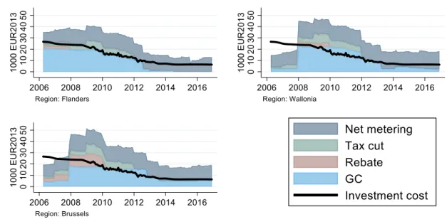
monthly inflation rate (set to a yearly rate of 2%), to capture the fact that the model is in real prices while GC benefits were guaranteed at nominal prices. We use the same specification for Brussels (𝛿!"#! ) and Wallonia (𝛿 !"#! ) until the reform of March 2014. We change it for Wallonia after this reform: we set 𝛿!"#! = (1 − 𝜋)𝛿 since the benefits were then based on capacity and not on actual production. 2.2.2 Evolution of the benefits of the PV subsidy programs Figure 1 shows the evolution of the various components of the benefits of the PV subsidy programs in the three regions, for a representative 4 kWp system. The benefits, 𝑏!"#!"#$%", 𝑏!"!"#$%! , 𝑏
!"#!"#$"#"% and 𝑏!"#!", are measured in present value terms based on the
methodology of section 2.2.1 (shaded areas). They are compared with the upfront investment price (black line). According to Figure 1, the upfront investment price has been continuously declining.8
For all three regions, the benefits from the rebate (red) and tax credits (green) were relatively small and were only present in the early years. The main part of the benefits came from the GCs (blue) and the net metering system (gray). Both started off very high in the early years. 7 The grid fee did not apply in the early years. But when it was introduced, it immediately applied to all PV installations, even those installed before the introduction.
8 Note that prices before 2009 should be interpreted with caution as they are predictions, based on a
The benefits from the GCs decreased over the period, though at a different pace between the regions. In Flanders (top left), the GC benefits were almost eliminated during 2012. In Wallonia (top right), the GC benefits also dropped considerably, though remained in place until the end. Also in Brussels, the GCs remained in place until the end of our data. An increasing electricity price made the net metering benefits increase steadily over time, except for the introduction of the grid fee in Flanders in 2015. Because of the decline in PV prices and other benefits, its relative importance in the investment decision increased substantially.
Figure 1. Evolution of the components of the subsidy programs (4KWp system)
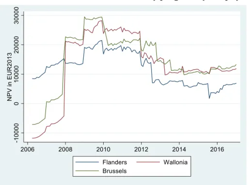
Figure 2 directly compares the regional evolution of the net present value, i.e. the difference between the present value of the future benefits and the investment price (𝑁𝑃𝑉!"# = 𝑏!"#− 𝑝!"). It again considers a 4 kWp system. In Flanders (blue line) the NPV was immediately positive with the introduction of the generous GC policy. It then further increased when investment costs went down (gradually) and the federal tax cut policy became more beneficial (2009-2011), but it dropped rather drastically in 2012 when changes in GC prices were implemented. Note however that it did remain positive over the entire period. In Wallonia and Brussels, the generous GC policy kicked off only in 2008, explaining the negative values in 2006 and 2007. Since then, the NPV in these regions has always been higher than in Flanders.
Figure 2. Evolution of the NPV of the subsidy programs (4 kWp system)
In sum, Figures 1 and 2 show that the structure of the subsidy programs was similar for the three regions, in the sense of showing a comparable emphasis on production subsidies in the form of GCs and net metering, with a faster fade-out of the GCs. But the timing and the magnitudes differed. Flanders started off earlier at very generous levels, but also eliminated the GCs more quickly and made the net metering less attractive through the introduction of a grid fee.
3 The impact of the subsidy programs on PV adoption
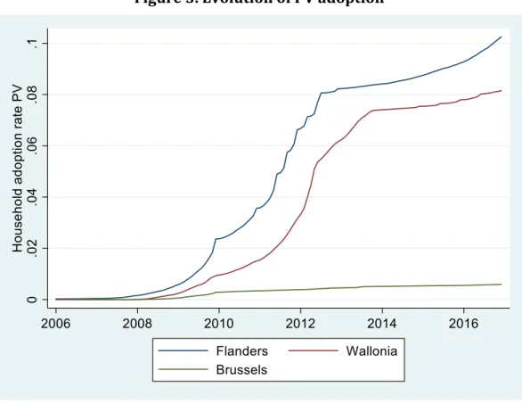
How did the generous subsidy programs affect the adoption of solar PVs? Before addressing this question in further detail, it is informative to have a first look at the aggregate numbers for the three regions. Figure 3 shows the evolution of the total adoption rate, i.e. the cumulative number of PV installations divided by the number of households.9 The total adoption rate has grown sharply in both Flanders and Wallonia, while it remained limited in urban Brussels. Wallonia started slightly later than Flanders, as may be expected because it introduced the programs at a later point. New adoptions were especially high during 2009-2012 when the NPV of investment reached the highest levels. Adoption rates in both regions reached a first plateau in 2012-2013, when the generous GC system was phased out. After that, the adoption rate gradually started to grow again, especially in Flanders. This is consistent with the recent evolution in the NPV. While the introduction of the grid fee in Flanders lowered it initially, the increase in electricity prices quickly made up for this. In Wallonia, the lower observed growth might be explained by the uncertainty surrounding the possible adoption of a prosumer fee, that was constantly debated, but only implemented in October 2020.
9 Throughout this paper, we make use of data from the Census of 2011 (https://census2011.fgov.be/) to
Figure 3. Evolution of PV adoption In sum, the large subsidy programs appear to have resulted in massive adoption of new PVs. As of today, despite a relatively low solar irradiance, the penetration of solar panels is important with 10.25% of the households equipped with solar PVs in Flanders, 0.6% in Brussels and 8.15% in Wallonia at the end of 2016. The graph also shows that the announced changes in GC subsidies were anticipated by the households. We indeed observe kinks in the curves, especially in Flanders, corresponding to announced drops in GC subsidies. Prospective adopters anticipated their investments to benefit from the most generous PV subsidies, leading to spikes and drops in adoption just before and after a policy change.
In the rest of this section, we explore in more detail how the programs have affected adoption. In subsection 3.1 we estimate a descriptive model that explains how differences in adoption across the regions can (partly) be attributed to differing local market demographics (e.g. urbanized areas such as most of the Brussels region are less suited for rooftop PV modules). We estimate the model at the yearly level, to also investigate the impact of the main changes in financial incentives. In subsection 3.2, we explore the role of financial incentives in more depth. We use a dynamic model of technology adoption, where households trade off upfront costs against future benefits, while taking into account future investment opportunities. In the next section 4, we then discuss how the massive adoption has imposed strong financing challenges given the generosity of the system.
3.1 The determinants of PV adoption: a descriptive approach
In this subsection, we propose a descriptive model to explain the determinants of adoption and have a first idea on the role of the GC policy.
3.1.1 Model and data
We are interested in explaining the number of new PV adopters, 𝑃𝑉!", with a panel data set of local municipalities 𝑚 and years 𝑡. We observe this information for 11 years (2006-2016) for each of the 589 municipalities of Belgium, of which 308 are located in Flanders (region 𝑐 = 𝐹), 262 in Wallonia (𝑐 = 𝑊), and the remaining 19 in Brussels (𝑐 = 𝐵). The local determinants of adoption, 𝑥!, are time-invariant socioeconomic variables (retrieved for 2011): the number of households, population density, income, education, percentage of male and foreigners, percentage of homeowners (versus renters), household size, house size (number of rooms) and year of construction of the house. In addition, we include the present value of the GC benefits 𝑏!"!" (as the maximum
value of a 4kWp system within a year). This benefit variable has been quantitatively the most important and it also shows most variation over time.
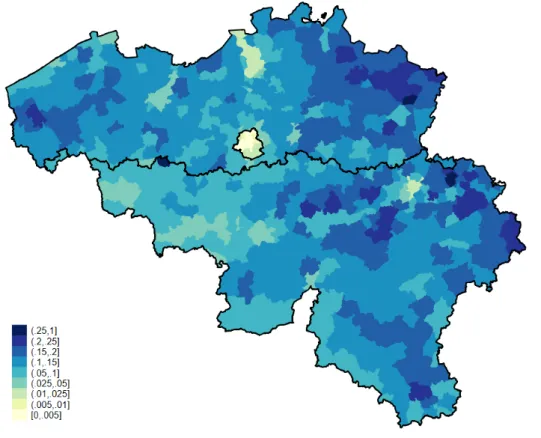
We observe large time and cross-sectional variation. Figure 3 showed that adoption rates increased substantially over time, probably due to differences in subsidization policies and the drop in investment costs. Figure 4 presents a map of adoption rates at the end of our sample, and shows that there is also large cross-sectional variation. Table 1 presents the descriptive statistics we use for the analysis. Figure 4: PV adoption (in % of households) by municipality in December 2016
𝐓𝐚𝐛𝐥𝐞 𝟏: 𝐃𝐞𝐬𝐜𝐫𝐢𝐩𝐭𝐢𝐯𝐞 𝐬𝐭𝐚𝐭𝐢𝐬𝐭𝐢𝐜𝐬
Mean Sd Min Max
PV adoptions (count by year) 61.646 100.366 0 1,484 log(households) 8.515 0.893 3.555 12.358 Log(population density) 5.733 1.158 3.215 10.100 Income group 2 0.200 0.400 0 1 Income group 3 0.200 0.400 0 1 Income group 4 0.200 0.400 0 1 Income group 5 0.200 0.400 0 1 % home owned 0.731 0.096 0.252 0.911 % higher education 0.308 0.076 0.127 0.592 % male 0.493 0.009 0.454 0.553 % foreign 0.068 0.074 0.009 0.497 Average household size 2.410 0.146 1.658 2.802 Average year of construction 1,962.502 11.121 1,931.096 1,982.188 Number of rooms 5.867 0.400 4.202 7.184 Wallonia 0.445 0.497 0.000 1.000 Brussels 0.032 0.177 0.000 1.000 GC (in 1000 EUR) 11.199 8.495 0.000 23.502 Total of 6,479 observations (589 municipalities x 11 years). Similar to De Groote, Pepermans and Verboven (2016), we assume that the number of new PV adopters, 𝑃𝑉!", has an exponential conditional mean function: 𝐸 𝑃𝑉!" |𝑥!, 𝑐, 𝑡, 𝑏!"!" = 𝑒𝑥𝑝 𝑥 !𝛽 + 𝛾!𝑏!"!"+ 𝐹𝐸! + 𝐹𝐸! ,
where 𝐹𝐸! represents region fixed effects, and 𝐹𝐸! captures a full set of year fixed effects, so the impact of the GC benefit variable 𝑏!"!" is identified from variation that is
specific to each region. We estimate the model using a Poisson pseudo-maximum-likelihood estimator (Silva and Tenreyro, 2006).10 3.1.2 Empirical results Table 2 presents the empirical results of five specifications. 10 A linear regression with 𝑙𝑛 𝑃𝑉 !" as the dependent variable gave comparable results.
Table 2. Descriptive model results
(1) (2) (3) (4)
Base Demographics GC Remove early
years log(households) 0.633*** 0.987*** 0.987*** 0.987*** (0.031) (0.028) (0.028) (0.028) Log(population density) -0.155*** -0.155*** -0.156*** (0.020) (0.020) (0.020) Income group 2 0.219*** 0.219*** 0.219*** (0.064) (0.064) (0.063) Income group 3 0.299*** 0.299*** 0.301*** (0.073) (0.073) (0.073) Income group 4 0.297*** 0.297*** 0.300*** (0.076) (0.076) (0.076) Income group 5 0.280*** 0.280*** 0.283*** (0.082) (0.082) (0.082) % home owned 1.153*** 1.153*** 1.170*** (0.287) (0.287) (0.285) % higher education -0.922*** -0.922*** -0.972*** (0.262) (0.262) (0.259) % male 8.866*** 8.866*** 8.797*** (2.141) (2.141) (2.119) % foreign -1.178*** -1.178*** -1.157*** (0.327) (0.327) (0.324) Average household size 0.289** 0.289** 0.282** (0.138) (0.138) (0.138) Average year of construction 0.020*** 0.020*** 0.019*** (0.002) (0.002) (0.002) Number of rooms 0.105** 0.105** 0.102** (0.049) (0.049) (0.049) Wallonia -0.346*** 0.258*** 0.563*** 0.627*** (0.034) (0.047) (0.050) (0.052) Brussels -2.463*** -0.920*** -1.857*** -1.543*** (0.129) (0.155) (0.212) (0.214) GC in Flanders (in 1000 EUR) 0.093*** 0.075*** (0.005) (0.006) GC in Wallonia (in 1000 EUR) 0.046*** 0.030*** (0.004) (0.005) GC in Brussels (in 1000 EUR) 0.137*** 0.098*** (0.013) (0.014)
Year fixed effects (base=2016) YES YES YES YES Sample period 2006-2016 2006-2016 2006-2016 2009-2016 Constant -1.344*** -48.922*** -49.072*** -48.423*** (0.275) (3.545) (3.546) (3.502) Observations 6,479 6,479 6,479 4,712
Descriptive model on total count of PVs in each year and municipality. Robust standard errors in parentheses, clustered within municipality. Estimates from Poisson Pseudolikelihood estimator. ***
p<0.01, ** p<0.05, * p<0.1
Specification (1) includes only the log of the number of households. This variable has a positive effect, but the estimated coefficient of 0.633 is significantly less than 1, suggesting that new adoptions increases less than proportionally with the number of households. Specification (2) incorporates the demographic variables 𝑥!. This results in a coefficient for the number of households that does not differ significantly from 1, implying an intuitive proportional relationship between new adopters and the number of households. The estimated coefficients of the socio-economic variables have the expected sign. For example, adoption is lower in more densely populated (urbanized) markets. It is higher in markets from the higher income groups (compared with the 20 percent lowest income group), in markets with a large fraction of homeowners, and with large houses and household sizes. The regional dummies (relative to the base Flanders) show some interesting effects. The coefficient for the Brussels region becomes much smaller, implying that the demographics (notably population density) explain a substantial part of the observed low adoptions in Brussels. The coefficient for Wallonia also becomes smaller in absolute value, but it changes sign. So after controlling for the demographics Wallonia had a higher propensity to adopt than Flanders.
Specifications (3) and (4) of Table 2 include the present value of the GC benefits, 𝑏!"!", as
an explanatory variable. The year fixed effects then capture common effects, such as the federal tax cut policies or the investment price of PVs. Hence, (3) and (4) identify the effect of the GC benefits from within-region time variation.
According to specification (3), an increase in the net present value of GCs by 1000 EUR raises the number of adoptions 9.3% in Flanders, 4.6% in Wallonia, and 13.7% in Brussels. Specification (4) restricts the sample to 2009-2016, to capture the possibility that in the early years (2006-2008) households may not have been aware of the policy, or postponed their adoption to the time when prices dropped sufficiently. The estimated effects remain similar but become slightly smaller (respectively, 7.5%, 3.0% and 9.8%). For both (3) and (4), the higher estimated effect in Flanders than in Wallonia may be because GCs have a fixed price in Flanders, while their price fluctuates in Wallonia and this implies more uncertainty to investors.11 Alternatively, it may be the case that households in Flanders are overall more price sensitive (to both GCs and the investment costs). We will further investigate this in the dynamic model.
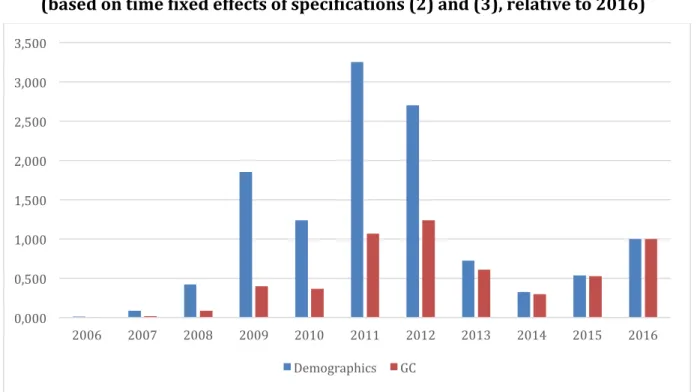
To illustrate further the importance of the GC policies, Figure 5 compares the estimated year fixed effects for specifications (2) and (3) in index form relative to 2016.12 According to (2), which does not control for the GCs, there are very large fluctuations in the number of adopters (blue bars). At the start of the subsidization policy in Flanders (2006), the number of adoptions was still very low at only 1.3% of the level in 2016. In 2009-2012, when GC subsidies were high in every region, the number of adoptions was up to 3.2 times larger than in 2016. In contrast, according to specification (3), which 11 Our NPV estimates are based on the GC price at the adoption date. In Wallonia, market prices were continuously declining due to an oversupply of certificates. The nominal GC price falls from 89.95€ in 2007 to 68.14€ in 2016. Hence, our estimated present value of the GCs is higher than the true value on investment.
controls for the impact of the GCs, the fluctuations become much smaller. The adoptions in 2011 and 2012, when the subsidy programs were the most generous, are now more comparable to 2016.13 The gradual increase after 2013 may be due to the continuous improvement of PV technology, implying lower prices for a given capacity. Figure 5. Evolution of PV adoption: without and with accounting for GC policy (based on time fixed effects of specifications (2) and (3), relative to 2016)
These findings are suggestive of the role of the GC policy in explaining the adoption levels, but they need to be interpreted with proper caution. First, the descriptive model is not motivated by economic theory: it does not explicitly model how households trade off upfront investment costs with future benefits. This makes it difficult to include all sources of costs and benefits and obtain reliable estimates of their effect, especially when some of them show little variation in the data. Second, the data were aggregated at the yearly level, while Figure 3 showed that there is also rich within-year variation in adoptions. A model with forward-looking agents is crucial to exploit this variation as households often postpone their adoption to the last month before a regime drop. Looking only at the current period investment opportunities is therefore not appropriate to explain their behavior at such a high frequency. Third, the analysis was done for a representative PV model of 4kWp, but there is relevant variation in the costs and benefits of different capacity levels, which may influence the timing of adoption decisions. To take these into account, the next subsection considers a dynamic adoption model.
3.2 The dynamics of PV adoption
Our dynamic model follows De Groote and Verboven (2019). It explicitly takes into account two trade-offs households face. First, it considers the investment trade-off by comparing the investment costs that households pay for their installation with the 0,000 0,500 1,000 1,500 2,000 2,500 3,000 3,500 2006 2007 2008 2009 2010 2011 2012 2013 2014 2015 2016 Demographics GC
expected investment benefits (which largely result from government policy). Second, it takes into account a dynamic trade-off by modeling households as forward-looking agents who have expectations about future costs and benefits and wait for the ideal time to adopt.
The estimates from this model will enable us to derive the households’ general sensitivity to monetary incentives, as well as how they value benefits (and therefore subsidies) relative to upfront investment costs, and this effect can be estimated for each region.
3.2.1 Dynamic model and data
We consider a model at the level of the region 𝑐 (rather than the individual municipalities as in the static model).14 In a given month 𝑡 a household 𝑖 located in region 𝑐 may either choose not to adopt a PV, 𝑗 = 0, or choose to adopt one of the available PV alternatives, 𝑗 = 1, … , 𝐽, i.e. the different capacity sizes of the PVs in our setting. A key feature of the model is that the adoption decision (𝑗 ≠ 0) is a terminating action. Not adopting (𝑗 = 0) gives the option to adopt at a later period, when the prices may have decreased, or when the financial benefits may have changed. Households can differ in their valuation of a PV. In each month 𝑡 a household 𝑖 located in region 𝑐 obtains a random taste shock for alternative 𝑗, 𝜀!"#$, assumed to follow a type 1 extreme value distribution. Conditional value of adoption
Let 𝑣!"# be the expected discounted utility of adoption, net of the taste shock 𝜀!"#$. We can write this as follows:
𝑣!"# = 𝑥!"#𝛾! − 𝛼!𝑝!"+ 𝛼!𝜃!𝑏!"#+ 𝜉!"#, 𝑗 = 1, … , 𝐽
where 𝑥!"# is a vector of characteristics of alternative 𝑗 at period 𝑡 in region 𝑐, 𝑝!" is the
upfront investment cost and 𝑏!"# is the total discounted benefits for adoption at time 𝑡. We described the various components of 𝑏!"# earlier in section 2.2.1. The term 𝜉!"# is an unobserved product characteristic, known to the household but not to the econometrician.
The parameter 𝛼!, which is allowed to be specific to each region 𝑐, measures the
households’ sensitivity to the upfront investment price. The parameter 𝜃! captures the households’ relative valuation of future financial benefits. If 𝜃! = 1, households value future benefits in the same way as upfront investment costs. If 𝜃! = 0, households fully ignore future benefits.
Conditional value of no adoption
Let 𝑣!!! be the expected discounted utility of not adopting PV (𝑗 = 0). We can write this as follows:
𝑣!!! = 𝑢!!! + 𝛿𝐸!𝑉!"!!,
where 𝑢!!! is the utility derived from not adopting PV at time 𝑡, 𝑉!"!! is the ex-ante value function, i.e. the continuation value from behaving optimally from period 𝑡 + 1
14 De Groote and Verboven (2019) show that accounting for local market heterogeneity changes little to the estimates that explain (average) sensitivity to prices and subsidies.
onwards, before taste shocks are revealed. The parameter 𝛿 is the monthly discount factor corresponding to an annual interest rate of 3%.15 Linear regression equation Following Scott (2013) and De Groote and Verboven (2019), we can derive the following linear regression equation (see Appendix 2): ln 𝑆!"#− ln 𝑆!!!− 𝛿 ln 𝑆!!!!! = 𝑥!"#− 𝛿𝑥!!!!! 𝛾! −𝛼!(𝑝!"− 𝛿𝑝!!!!) + 𝛼!𝜃!(𝑏!"#− 𝛿𝑏!!!!!) + 𝜉!"#− 𝛿(𝜉!!!!!− 𝜂!"),
where 𝜂!" ≡ 𝑉!"!!− 𝐸!𝑉!"!! is an expectation error, and 𝑆!"# is the observed market share of alternative 𝑗, i.e. the number of new adopters of 𝑗 relative to the potential number of households who did not yet adopt a PV system.
This regression equation is essentially a dynamic Euler equation. Note that the error term of the regression consists of both the unobserved characteristics and the expectation error. If the price is endogenous (correlated with unobserved characteristics), we could estimate this using instrumental variables. We will instead treat prices as exogenous, conditional on a set of fixed effects for each capacity choice and each year. We also do a robustness check with a full set of capacity/year fixed effects. Intuitively, this assumption means that any monthly price variation within a year is not driven by local demand forces, but rather by global market conditions, which appears to be reasonable given the small size of Belgium.16
To estimate the model we make use of our data on new PV installations for each capacity level 𝑗, region 𝑐 and month 𝑡 and on the upfront investment price 𝑝!", and we measure the future benefits as 𝑏!"# = 𝑏!"#!"#$%&'+ 𝑏!"!"#$%!+ 𝑏 !"#!"#$"#"%+ 𝑏!"#!". In a sensitivity analysis, we also conduct a more flexible specification, where the non-GC benefit terms enter as separate terms. 3.2.2 Empirical results
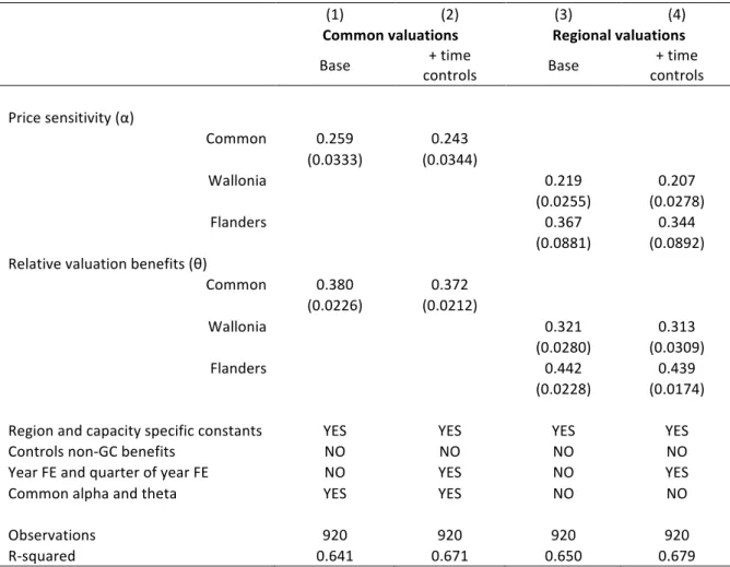
Table 3 presents the empirical results of the dynamic model, for four different specifications. The total number of observations is 920, consisting of 5 capacity alternatives, observed in 2 regions17 over 92 months (i.e. 7 years and 8 months from May 2009 to December 2016). The “common valuations” specifications (1) and (2) assume that the regions have a common valuation of price (𝛼! = 𝛼) and a common relative valuation of future benefits (𝜃! = 𝜃). The “regional valuations” specifications (3) and (4) allow these valuations to be specific to the regions. The odd-numbered specifications include only capacity fixed effects, while the even-numbered specifications also include year fixed effects and quarter fixed effects.
15 Alternatively, as in De Groote and Verboven (2019), we also estimated a (non-linear) specification that
imposes 𝜃! = 1, and estimates 𝛿 as the households’ implicit discount factor (possibly region-specific),
both in the conditional value function of 𝑗 = 0 and in the calculation of benefits 𝑏!"#. We then derive similar conclusions about price sensitivity and the valuation of benefits.
16 We also replicate De Groote and Verboven (2019) who use Chinese module prices as an instrument with the data for Flanders until 2012. We find similar results when prices are assumed to be exogenous. 17 We do not include Brussels in this dynamic model because adoption was too low to be considered.
Table 3. Empirical results from dynamic adoption model
(1) (2) (3) (4)
Common valuations Regional valuations
Base controls + time Base controls + time
Price sensitivity (α) Common 0.259 0.243 (0.0333) (0.0344) Wallonia 0.219 0.207 (0.0255) (0.0278) Flanders 0.367 0.344 (0.0881) (0.0892) Relative valuation benefits (θ) Common 0.380 0.372 (0.0226) (0.0212) Wallonia 0.321 0.313 Flanders (0.0280) (0.0309) 0.442 0.439 (0.0228) (0.0174)
Region and capacity specific constants YES YES YES YES
Controls non-GC benefits NO NO NO NO
Year FE and quarter of year FE NO YES NO YES
Common alpha and theta YES YES NO NO
Observations 920 920 920 920 R-squared 0.641 0.671 0.650 0.679 Results from linear regression on market share inversion for two regions (Flanders and Wallonia) over five capacity choices and 92 months (May 2009-December 2016). Robust standard errors in parentheses. Observations clustered within time period. Standard errors theta obtained using delta method.
The common valuation specifications (1) and (2) show that households have a significant general price sensitivity (𝛼), and that the relative valuation of future benefits compared with upfront costs is low (𝜃 close to 0.4). This suggests stronger time discounting than found by De Groote and Verboven (2019), which applied to a shorter period (up to 2012) and only the region of Flanders. They found that consumers are willing to pay only 0.5 Euro upfront for one extra euro of future subsidy benefits (at an interest rate of 3%). The results in specifications (1) and (2) show slightly higher discounting.
In our descriptive model (section 3.1), we found a smaller impact of GC subsidies in Wallonia, compared to other regions. The dynamic model allows us to investigate if this follows from a higher sensitivity to monetary incentives (𝛼) or a lower relative valuation of benefits compare to investment costs (𝜃). Specifications (3) and (4) allow for these regional differences and show evidence of both: households in Flanders are more price-sensitive (𝛼! > 𝛼!) and undervalue the benefits to a lesser extent (𝜃! > 𝜃!). The latter seems to suggest that households in Wallonia may be less forward-looking. This higher discounting of the GC benefits in Wallonia compared to Flanders might be explained by the different design of the GC schemes guaranteeing a fixed price for the GC in Flanders while guaranteeing a fixed tradable GC allowance in Wallonia. The relative uncertainty
on the evolution of the GC price may imply a higher discounting of future benefit in Wallonia.18 However, it is also possible that this is due to the different policy context, which may have created confusion or political uncertainty.
In sum, these findings show that households show significant sensitivity to monetary incentives, especially so in Flanders. After controlling for this difference in sensitivity to monetary reasons to adopt, it appears that the design of the GC policy was relatively more effective in Flanders than in Wallonia. Households in Wallonia more strongly undervalue financial benefits, including the GC subsidies, but they were so generous that they still led to massive adoption in both regions.
4 Financing issues of the policies and the political debate
The generous subsidies (documented in section 2) and the massive PV adoption (documented in section 3) implied substantial and increasing financial costs to society. This has subsequently led to intense political debate and subsidies to solar PV became a political issue. In this section, we will discuss the financing issues and subsequent political debate. This debate mainly focused on the financing of the GC system and the net metering, and not on the rebates (which were relatively small and only in the first years). 4.1 Financing issues 4.1.1 Investment support The investment rebates and the tax credits were financed by the general budget of the regions and the federal government, respectively. This involved only a limited debate because it concerned relatively small amounts that were phased out very quickly as we have seen. Furthermore, financing through the general budget is less visible as it is just a small part of the overall government budget. 4.1.2 GC system The main cost overrun came from the cost of the GC mechanism, especially the generous schemes offered at the early stages. High adoption and generous production subsidies have generated an unanticipated green certificate debt in both Flanders and Wallonia.19 This GC debt is an accumulated amount of subsidies that were paid to the beneficiary households (the prosumers) but which were not yet paid by society (through increased electricity prices or taxes). Around 2012, it became apparent that the GC mechanism was extremely costly and that this cost would be passed through to consumers. The financing of the GC debt became a political issue. Given that each region had specific measures to support PVs, it is important to clarify how this debt was generated and how it was financed.
18 Nicolini and Tavoni (2017) document that feed-in-tariffs guaranteeing a fixed payment per kWh produced (like the GC system in place in Flanders for solar) are more effective than the tradeable green certicate mechanism to stimulate investment in renewables.
19 The government in charge clearly underestimated the high take-up rate and its consequences. For example, the bill in Flanders that introduced the policy stated an expected total capacity of 16,500 kWP by 2010 (Source: Flemish Parliament, piece 2188 (2003-2004)). By the end of 2009, and only looking at PVs <10kW, total capacity had already reached 260,398 kWp (15 times higher than the initial estimate). By the end of 2012, the end of the first phase of the GC policy, it had reached 1,046,164 kWp (63 times higher).
In Flanders, the public DSOs had the obligation to buy the GCs from the prosumers at a guaranteed price in their role of default buyers. The DSOs could then resell the GCs on the market to the retailers, who had quota obligations to sell an (increasing) share of green electricity. When the guaranteed price exceeds the market price, the DSOs are making losses when they resell GCs. These losses are important and continue to be accumulated because the GC rights are granted for a long period.
To finance this debt, Flanders imposed, in 2015, a flat tax on each consumption point. The amount of the tax increased with the level of consumption, but only to a small extent, which was the main critique in the public debate. The tax was substantial. Consumers with a consumption level <5MWh/year had to pay an additional €100. The tax was abolished from January 2018 on and replaced by a low fee of about €9 per year.20 The abolishment of this contentious tax21 came after a decision by the constitutional court on June 2017.
In Wallonia, prosumers received more GCs compared to producers of alternative sources of green energy. This high granting rate generated an excessive supply of GCs on the market i.e. the number of issued GCs exceeded, by large, the yearly quota.22 This had two consequences. First, the GC price dropped and is now close to the price floor. Second, the default buyer, the TSO, had to buy many GCs at the minimum guaranteed price.
Some of the excessive GCs bought by the TSO were cancelled and, therefore, no longer available on the market. In exchange, the TSO introduced a specific surcharge to the electricity consumers in Wallonia.23 This surcharge was insufficient to cover the full cost borne by the TSO, but the regional government did not want to increase further the energy price, i.e. it did not want a full pass-through of the cost. Instead, it bought back the additional GCs from the TSO. To that end, the government created a special purpose vehicle (SPV) which accumulated the GC debt to be passed on to future consumers. 4.1.3 Net metering The cost of net metering is essentially a lost income to the DSOs. The prosumers’ bill is based on their net consumption (consumption minus solar production). Consequently, their contribution to the network cost decreases and could be zero if their yearly production exceeds their yearly consumption.24
To recover their costs (mostly fixed), the DSOs have to adapt their tariffs. Flanders and Wallonia decided to impose a prosumer fee. This prosumer fee is based on the PV capacity (in kWp) and it is designed as a contribution of the prosumers to the grid cost. Brussels instead decided to stop net metering in 2020, also for PVs that were installed before. 20 Source: https://www.tijd.be/politiek-economie/belgie/vlaanderen/hoe-tommelein-de-turteltaks-van-100-naar-9-euro-doet-zakken/9935978.html (consulted on 21/09/2020).
21 This tax is known as the “Turteltaks”, after the name of the Flemish minister in charge of energy, Annemie Turtelboom who imposed it. The opposition against the tax eventually caused her to step down as minister. 22 See Gautier and Boccard (2015, 2019) for a detailed analysis of this market. 23 Currently the surcharge is equal to 13.82€/MWh. 24 This would not be the case with a net purchasing system that records and price separately the imports from the grid and the exports to the grid. For a comparison between net metering and net purchaisng see Gautier et al. (2018).
The imposition of grid fees on prosumers was an extremely contentious issue. It was seen by prosumers as an attempt by the governments to renegotiate their promises and lower ex-post the return on their investment. For these reasons, the earlier attempts to impose such a fee were (successfully) challenged in courts by some prosumers. In Flanders, the prosumer fee was introduced in January 2013 and canceled by the Court in November 2013. It was then reintroduced successfully in July 2015. In Wallonia, the prosumer fee was introduced in 2014 but canceled by the Court in June 2015 and, in practice, the fee was never applied (contrary to Flanders where the DSOs had to pay back the fee after the Court found it illegal). The regulator introduced a fee, in principle in January 2020, but the regional government opposed it. After long discussions, the fee will be applied in October 2020.
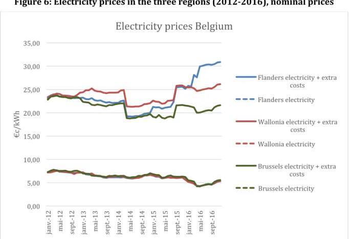
4.2 Evolution of electricity prices
The cost of the subsidies and the way they were financed translated into changes in electricity prices. The following figure show the evolution of the retail price of electricity for a representative consumer in Flanders, Wallonia and Brussels. Prices started to diverge from 2012, reflecting the different policy choices made by the regions, mainly to finance the support to green energy sources. As can be observed on the figure, the commodity price is almost the same in the three regions and the price differences mainly come from grid fees and surcharges to support green energy. The lower price in Brussels can be explained by the absence of a GC debt because of lower adoption. The difference between Flanders and Wallonia partially reflects the choice made in Wallonia to transfer a part of the GC debt to future consumers, while Flanders decided to pass most of the debt to current consumers.