Physical properties of the planetary systems WASP-45 and
WASP-46 from simultaneous multi-band photometry
?
S. Ciceri
1†, L. Mancini
1,2, J. Southworth
3, M. Lendl
4,5, J. Tregloan-Reed
6,3,
R. Brahm
7,8, G. Chen
9,10, G. D’Ago
11,12,22, M. Dominik
13, R. Figuera Jaimes
13,14,
P. Galianni
13, K. Harpsøe
15, T. C. Hinse
16, U. G. Jørgensen
15, D. Juncher
15,
H. Korhonen
15,17, C. Liebig
13, M. Rabus
1,7, A. S. Bonomo
2, K. Bott
18,19,
Th. Henning
1, A. Jord´
an
7,8, A. Sozzetti
2, K. A. Alsubai
20, J. M. Andersen
15,21,
D. Bajek
13, V. Bozza
12,22, D. M. Bramich
20, P. Browne
13, S. Calchi Novati
23,11,12?‡,
Y. Damerdji
24, C. Diehl
25,26, A. Elyiv
24,27,28, E. Giannini
25, S-H. Gu
29,30,
M. Hundertmark
15, N. Kains
31, M. Penny
32,15, A. Popovas
15, S. Rahvar
33,
G. Scarpetta
11,12,22, R. W. Schmidt
25, J. Skottfelt
35,15, C. Snodgrass
35,36, J. Surdej
24,
C. Vilela
3, X-B. Wang
29,30and O. Wertz
241Max Planck Institute for Astronomy, K¨onigstuhl 17, 69117 – Heidelberg, Germany
2INAF – Osservatorio Astrofisico di Torino, via Osservatorio 20, 10025 – Pino Torinese, Italy 3Astrophysics Group, Keele University, Staffordshire, ST5 5BG, UK
4Austrian Academy of Sciences, Space Research Institute, Schmiedlstrasse 6, 8042 Graz, Austria5Observatoire de Gen`eve, Universit´e de Gen`eve, Chemin des maillettes 51, 1290 Sauverny, Switzerland 6NASA Ames Research Center, Moffett Field, CA 94035, USA
7Instituto de Astrof´ısica, Pontificia Universidad Cat´olica de Chile, Av. Vicu˜na Mackenna 4860, 7820436 – Macul, Santiago, Chile 8Millennium Institute of Astrophysics, Av. Vicu˜na Mackenna 4860, 7820436 – Macul, Santiago, Chile
9Key Laboratory of Planetary Sciences, Purple Mountain Observatory, Chinese Academy of Sciences, Nanjing 210008, China 10Instituto de Astrof´ısica de Canarias, E-38205 La Laguna, Tenerife, Spain
11International Institute for Advanced Scientific Studies (IIASS), Via G. Pellegrino 19, 84019 – Vietri Sul Mare (SA), Italy 12Department of Physics “E. R. Caianiello”, University of Salerno, Via Giovanni Paolo II 132, Fisciano (SA) – 84084 13SUPA, University of St Andrews, School of Physics & Astronomy, North Haugh, St Andrews, Fife KY16 9SS, UK 14European Southern Observatory, Karl-Schwarzschild Straße 2, 85748 – Garching bei M¨unchen, Germany
15Niels Bohr Institute & Centre for Star and Planet Formation, University of Copenhagen, Øster Voldgade 5, 1350 – Copenhagen K, Denmark 16Korea Astronomy and Space Science Institute, 305-348 Daejeon, Republic of Korea
17Finnish Centre for Astronomy with ESO (FINCA), University of Turku, V¨ais¨al¨antie 20, FI-21500 Piikki¨o, Finland 18School of Physics, UNSW Australia, NSW 2052, Australia
19Australian Centre for Astrobiology, UNSW Australia, NSW 2052, Australia
20Qatar Environment and Energy Research Institute, Qatar Foundation, Tornado Tower, Floor 19, PO Box 5825, Doha, Qatar 21Department of Astronomy, Boston University, 725 Commonwealth Avenue, Boston, MA 02215, USA
22Istituto Nazionale di Fisica Nucleare, Sezione di Napoli, I-80126 Napoli, Italy
23NASA Exoplanet Science Institute, MS 100-22, California Institute of Technology, Pasadena CA 91125
24Institut d’Astrophysique et de G´eophysique, Universit´e de Li`ege, All´ee du 6 Aoˆut 17, Bˆat. B5C, Li`ege 1, 4000 Belgium
25Astronomisches Rechen-Institut, Zentrum f¨ur Astronomie, Universit¨at Heidelberg, Mnchhofstraße 12-14, D-69120 Heidelberg, Germany 26Hamburger Sternwarte, Universit¨at Hamburg, Gojenbergsweg 112, D-21029 Hamburg, Germany
27Dipartimento di Fisica e Astronomia, Universit di Bologna, Viale Berti Pichat 6/2, I-40127 Bologna, Italy
28Main Astronomical Observatory, Academy of Sciences of Ukraine, vul. Akademika Zabolotnoho 27, UA-03680 Kyiv, Ukraine 29Yunnan Observatories, Chinese Academy of Sciences, Kunming 650011, China
30Key Laboratory for the Structure and Evolution of Celestial Objects, Chinese Academy of Sciences, Kunming 650011,China 31Space Telescope Science Institute, 3700 San Martin Drive, Baltimore, MD 21218, USA
32Department of Astronomy, Ohio State University, McPherson Laboratory, 140 West 18th Avenue, Columbus, OH 43210-1173, USA 33Department of Physics, Sharif University of Technology, PO Box 11155-9161 Tehran, Iran
34Centre for Electronic Imaging, Dept. of Physical Sciences, The Open University, Milton Keynes MK7 6AA, UK 35Planetary and Space Sciences, Department of Physical Sciences, The Open University, Milton Keynes, MK7 6AA, UK 36Max Planck Institute for Solar System Research, Justus-von-Liebig-Weg 3, D-37077 G¨ottingen, Germany
2015 November 16
ABSTRACT
Accurate measurements of the physical characteristics of a large number of ex-oplanets are useful to strongly constrain theoretical models of planet formation and evolution, which lead to the large variety of exoplanets and planetary-system con-figurations that have been observed. We present a study of the planetary systems WASP-45 and WASP-46, both composed of a main-sequence star and a close-in hot Jupiter, based on 29 new high-quality light curves of transits events. In particular, one transit of WASP-45 b and four of WASP-46 b were simultaneously observed in four op-tical filters, while one transit of WASP-46 b was observed with the NTT obtaining a precision of 0.30 mmag with a cadence of roughly three minutes. We also obtained five new spectra of WASP-45 with the FEROS spectrograph. We improved by a fac-tor of four the measurement of the radius of the planet WASP-45 b, and found that WASP-46 b is slightly less massive and smaller than previously reported. Both plan-ets now have a more accurate measurement of the density (0.959 ± 0.077 ρJup instead
of 0.64 ± 0.30 ρJup for WASP-45 b, and 1.103 ± 0.052 ρJup instead of 0.94 ± 0.11 ρJup
for WASP-46 b). We tentatively detected radius variations with wavelength for both planets, in particular in the case of WASP-45 b we found a slightly larger absorption in the redder bands than in the bluer ones. No hints for the presence of an additional planetary companion in the two systems were found either from the photometric or radial velocity measurements.
Key words: stars: fundamental parameters – stars: individual: WASP-45 – stars: individual: WASP-46 – planetary systems
1 INTRODUCTION
The possibility to obtain detailed information on extraso-lar planets, using different techniques and methods, has re-vealed some unexpected properties that are still challenging astrophysicists. One of the very first was the discovery of Jupiter-like planets on very tight orbits, which are labelled hot Jupiters, and the corresponding inflation-mechanism problem (Baraffe et al. 2014, and references therein). To find the answers to this and other open questions, it is impor-tant to have a proper statistical sample of exoplanets, whose physical and orbital parameters are accurately measured.
One class of extrasolar planets, those which transit their host stars, has lately seen a large increase in the number of its known members. This achievement has been possi-ble thanks to systematic transit-survey large programs, per-formed both from ground (HATNet: Bakos et al. 2004; TrES: Alonso et al. 2004; XO: McCullough et al. 2005; WASP: Pol-lacco et al. 2006; KELT: Pepper et al. 2007; MEarth: Char-bonneau et al. 2009; QES: Alsubai et al. 2013; HATSouth: Bakos et al. 2013), and from space (CoRoT: Barge et al. 2008, Kepler : Borucki et al. 2011).
The great interest in transiting planets lies in the fact that it is possible to measure all their main orbital and phys-ical parameters with standard astronomphys-ical techniques and instruments. From photometry we can estimate the period, the relative size of the planet and the orbital inclination, whilst precise spectroscopic measurements provide a lower
? Based on data collected by the MiNDSTEp collaboration with
the Danish 1.54 m telescope, and on data observed with the NTT (under program number 088.C-0204(A)), 2.2m and Euler-Swiss Telescope all located at the ESO La Silla Observatory.
† E-mail: ciceri@mpia.de ‡ Sagan visiting fellow
limit for the mass of the planet (but knowing the inclina-tion from photometry the precise mass can be calculated) and the eccentricity of its orbit. Unveiling the bulk den-sity of the planets allows the imposition of constraints on, or differentiation between, the diverse formation and migra-tion theories which have been advanced (see Kley & Nelson 2012; Baruteau et al. 2014 and references therein).
Furthermore, transiting planets allow astronomers to investigate their atmospheric composition, when observed in transit or occultation phases (e.g. Charbonneau et al. 2002; Richardson et al. 2003). However, is also important to stress that, besides instrumental limitations, the characterisation of planets’ atmosphere is made difficult by the complexity of their nature. Retrieving the atmospheric chemical composi-tion may be hindered by the presence of clouds, resulting in a featureless spectrum (e.g. GJ 1214 b, Kreidberg et al. 2014).
In this work, we focus on two transiting exoplanet sys-tems: WASP-45 and WASP-46. Based on new photometric and spectroscopic data, we review their physical parameters and probe the atmospheres of their planets.
1.1 WASP-45
WASP-45 is a planetary system discovered within the Su-perWASP survey by Anderson et al. (2012) (A12 hereafter). The light curve of WASP-45, shows a periodic dimming (ev-ery P = 3.126 days) due to the presence of a hot Jupiter (radius 1.16+0.28−0.14RJup and mass 1.007 ± 0.053 MJup) that
transits the stellar disc. The host (mass of 0.909 ± 0.060 M and radius of 0.945+0.087−0.071R ) is a K2 V star with a higher
metallicity than the Sun ([Fe/H] = +0.36 ± 0.12). The study of the CaII H+K lines in the star’s spectra revealed weak emission lines, which indicates a low chromospheric activity.
1.2 WASP-46
WASP-46 is a G6 V type star (mass 0.956 ± 0.034 M , ra-dius 0.917 ± 0.028 R and [Fe/H] = −0.37 ± 0.13). A12 dis-covered a hot Jupiter (mass 2.101 ± 0.073 MJup and radius
1.310 ± 0.051 RJup) that orbits the star every 1.430 days on
a circular orbit. As in the case of WASP-45, weak emission visible in the CaII H+K lines indicates a low stellar activ-ity. Moreover, the WASP light curve shows a photometric modulation, which allowed the measurement of the rotation period of the star, and a gyrochronological age of the system of 1.4 Gyr. By observing the secondary eclipse of the planet, Chen et al. (2014) detected the emission from the day-side atmosphere finding brightness temperatures consistent with a low heat redistribution efficiency.
2 OBSERVATIONS AND DATA REDUCTION
A total of 29 light curves of 14 transit events of WASP-45 b and WASP-46 b, and five spectra of WASP-45 were obtained using four telescopes located at the ESO La Silla observa-tory, Chile. The details of the photometric observations are reported in Table 1.
The photometric observations were all performed with the telescopes in auto-guided mode and out of focus to min-imise the sources of noise and increase the signal to noise ra-tio (S/N). By spreading the light of each single star on many more pixels of the CCD, it is then possible to utilise longer exposure times without incurring saturation. Atmospheric variations, change in seeing, or tracking imprecision lead to changes in the position and/or size of the point spread func-tion (PSF) on the CCD and, according to the different re-sponse of each single pixel, spurious noise can be introduced in the signal. By obtaining a doughnut-shaped PSF that covers a circular region with a diameter from roughly 15 to 30 pixels, the small variations in position are averaged out and have a much lower effect on the photometric precision (Southworth et al. 2009).
1.2 m Euler-Swiss Telescope
The imager of the 1.2m Euler-Swiss telescope, EulerCam, is a 4000 × 4000 e2v CCD with a field of view (FOV) of 15.70× 15.70, yielding a resolution of 0.23 arcsec per pixel. Since its installation in 2010, EulerCam has been used intensively for photometric follow-up observations of planet candidates from the WASP survey (e.g. Hellier et al. 2011; Lendl et al. 2014), as well as for the atmospheric study of highly irradiated giant planets (Lendl et al. 2013). We observed one transit of WASP-45 b and two transits of WASP-46 b with EulerCam between June and September 2011 using a Gunn r’ fiter.
3.58 m NTT
One transit of WASP-46 b was observed with the New Tech-nology Telescope (NTT) on the 23 October 2011. The tele-scope has a primary mirror of 3.58 m and is equipped with an active optics system. The EFOSC2 instrument (ESO Faint Object Spectrograph and Camera 2), mounted on its
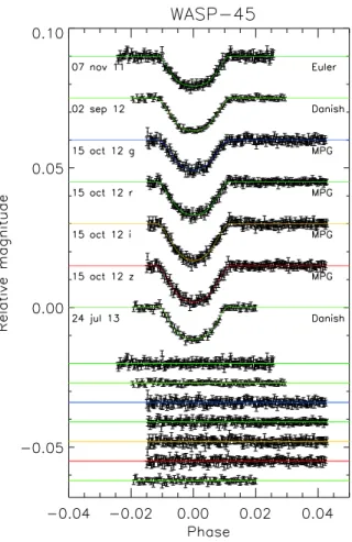
Figure 1. Phased light curves corresponding to four transits of WASP-45 b. The date and the telescope used for each transit event are indicated close to the corresponding light curve. Each light curve is shown with its best fit obtained with jktebop. The residuals relative to each fit are displayed at the base of the figure in the same order as the light curves. The curves are shifted along the y axis for clarity.
Nasmyth B focus, was utilised. The field of view of its Lo-ral/Lesser camera is 4.10 × 4.10
with a resolution of 0.12 arcsec per pixel. During the observation of the whole tran-sit, only a small region of the CCD, including the target and some reference stars, was read out in order to diminish the readout time and increase the sampling. The filter used was a Gunn g (ESO #782).
1.54 m Danish Telescope
Two transits of WASP-45 b and three of WASP-46 b were ob-served with the 1.54 m Danish Telescope, using the DFOSC (Danish Faint Object Spectrograph and Camera) instru-ment mounted at the Cassegrain focus. The instruinstru-ment, now used exclusively for imaging, has a CCD with a FOV 13.70× 13.70 and a resolution of 0.39 arcsec per pixel. The CCD was windowed and a Bessell R filter was used for all the transits.
Table 1. Details of the transit observations presented in this work. Nobsis the number of observations, Texpis the exposure time, Tobs
is the observational cadence, and ‘Moon illum.’ is the fractional illumination of the Moon at the midpoint of the transit. The triplets of numbers in the Aperture radii column correspond to the inner radius of the circular aperture (star) and outer radii of the ring (sky) selected for the photometric measurements.aThe aperture radii of the Euler-Swiss light curves are referred to the target aperture and
are expressed in arcsec.
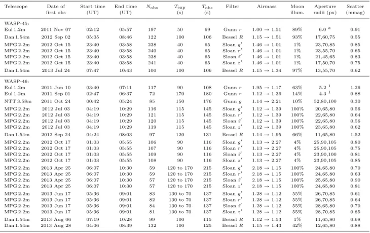
Telescope Date of Start time End time Nobs Texp Tobs Filter Airmass Moon Aperture Scatter
first obs (UT) (UT) (s) (s) illum. radii (px) (mmag) WASP-45:
Eul 1.2m 2011 Nov 07 02:12 05:57 197 50 69 Gunn r 1.00 → 1.51 89% 6.0a 0.91 Dan 1.54m 2012 Sep 02 05:05 08:46 122 100 106 Bessel R 1.15 → 1.51 93% 17,60,75 0.55 MPG 2.2m 2012 Oct 15 23:40 03:58 238 40 65 Sloan g0 1.46 → 1.01 1% 23,70,85 0.85 MPG 2.2m 2012 Oct 15 23:40 03:58 240 40 65 Sloan r0 1.46 → 1.01 1% 23,55,70 0.65 MPG 2.2m 2012 Oct 15 23:40 03:58 238 40 65 Sloan i0 1.46 → 1.01 1% 21,45,65 0.83 MPG 2.2m 2012 Oct 15 23:40 03:58 241 40 65 Sloan z0 1.46 → 1.01 1% 17,50,70 0.75 Dan 1.54m 2013 Jul 24 07:47 10:43 100 100 106 Bessel R 1.15 → 1.34 97% 13,55,70 0.62 WASP-46:
Eul 1.2m 2011 Jun 10 03:40 07:11 117 90 108 Gunn r 1.95 → 1.17 63% 5.21 1.26 Eul 1.2m 2011 Sep 01 02:47 06:37 72 170 180 Gunn r 1.12 → 1.36 14% 4.31 0.88
NTT 3.58m 2011 Oct 24 00:42 05:24 85 150 176 Gunn g 1.14 → 2.21 10% 52,80,100 0.30 MPG 2.2m 2012 Jul 03 04:19 10:29 116 115 145 Sloan g0 1.12 → 1.39 100% 20,65,80 0.56 MPG 2.2m 2012 Jul 03 04:19 10:29 121 115 145 Sloan r0 1.12 → 1.39 100% 22,65,80 0.64 MPG 2.2m 2012 Jul 03 04:19 10:29 120 115 145 Sloan i0 1.12 → 1.39 100% 22,65,80 0.56 MPG 2.2m 2012 Jul 03 04:19 10:29 119 115 145 Sloan z0 1.12 → 1.39 100% 23,65,80 0.62 Dan 1.54m 2012 Sep 24 04:24 08:03 97 120 131 Bessel R 1.14 → 1.95 66% 11,65,80 1.52 MPG 2.2m 2012 Oct 17 01:03 05:55 106 90 116 Sloan g0 1.13 → 2.27 4% 25,90,105 0.80 MPG 2.2m 2012 Oct 17 01:03 05:55 107 90 116 Sloan r0 1.13 → 2.27 4% 25,90,105 0.75 MPG 2.2m 2012 Oct 17 01:03 05:55 109 90 116 Sloan i0 1.13 → 2.27 4% 23,90,100 0.81 MPG 2.2m 2012 Oct 17 01:03 05:55 108 90 116 Sloan z0 1.13 → 2.27 4% 23,90,105 0.85 MPG 2.2m 2013 Apr 25 06:07 10:30 59 120 to 170 215 Sloan g0 2.18 → 1.15 100% 24,65,80 0.70 MPG 2.2m 2013 Apr 25 06:07 10:30 59 120 to 170 215 Sloan r0 2.18 → 1.15 100% 24,65,80 0.63 MPG 2.2m 2013 Apr 25 06:07 10:30 57 120 to 170 215 Sloan i0 2.18 → 1.15 100% 25,65,80 0.90 MPG 2.2m 2013 Apr 25 06:07 10:30 57 120 to 170 215 Sloan z0 2.18 → 1.15 100% 24,65,80 0.81 MPG 2.2m 2013 Jun 17 05:36 09:01 83 130 to 70 137 Sloan g0 1.28 → 1.12 55% 26,70,85 0.61 MPG 2.2m 2013 Jun 17 05:36 09:01 82 130 to 70 137 Sloan r0 1.28 → 1.12 55% 26,70,85 0.64 MPG 2.2m 2013 Jun 17 05:36 09:01 84 130 to 70 137 Sloan i0 1.28 → 1.12 55% 28,65,80 0.70 MPG 2.2m 2013 Jun 17 05:36 09:01 81 130 to 70 137 Sloan z0 1.28 → 1.12 55% 28,70,85 0.85 Dan 1.54m 2013 Aug 06 07:19 10:28 99 100 115 Bessel R 1.12 → 1.53 1% 11,65,80 0.68 Dan 1.54m 2013 Aug 28 04:06 08:39 132 100 125 Bessel R 1.15 → 1.43 42% 12,65,80 0.88
2.2 m MPG Telescope - GROND
The 2.2 m MPG Telescope holds in its Coud´e-like focus the GROND (Gamma Ray Optical Near-infrared Detector) in-strument (Greiner et al. 2008). GROND is a seven channel imager capable of performing simultaneous observations in four optical bands (g0, r0, i0, z0, similar to Sloan filters) and three near-infrared (NIR) bands (J , H, K). The light, split into different paths using dichroics, reaches two different sets of cameras. The optical cameras have 2048×2048 pixels with a resolution of 0.16 arcsec per pixel. The NIR cameras have a lower resolution 0.60 arcsec per pixel, but a larger FOV of 100× 100
(almost double the optical ones). The primary goal of GROND is the detection and follow-up of the optical/NIR counterpart of gamma ray bursts, but it has already proven to be a great instrument to perform multicolour, simulta-neous, photometric observations of planetary-transit events (e.g. Mancini et al. 2013b; Southworth et al. 2015). With this instrument, we observed one transit event of the planet WASP-45 b and four of WASP-46 b.
The exposure time must be the same for each optical camera, and is also partially constrained by the NIR expo-sure time chosen. We therefore decided to fix the expoexpo-sure time to that optimising the r0-band counts (generally higher than in the other bands) in order to avoid saturation.
2.2 m MPG Telescope - FEROS
The 2.2 m MPG telescope also hosts FEROS (Fibre-fed Ex-tended Range Optical Spectrograph). This ´echelle spectro-graph covers a wide wavelength range of 370 nm to 860 nm and has an average resolution of R = 48 000 ± 4 000. The precision of the radial velocity (RV) measurements obtained with FEROS is good enough (> 10 m s−1) for detecting and confirming Jupiter-size exoplanets (e.g. Penev et al. 2013; Jones et al. 2015). Simultaneously to the science observa-tions, we always obtained a spectrum of a ThAr lamp in order to have a proper wavelength calibration. Five spectra of WASP-45 were obtained with FEROS.
2.1 Data reduction
For all photometric data, a suitable number of calibration frames, bias and (sky) flat-field images, were taken on the same day as the observations. Master bias and flat-field im-ages were created by median-combining all the individual bias and flat-field images, and used to calibrate the scien-tific images.
With the exception of the EulerCam data, we then ex-tracted the photometry from the calibrated images using a version of the aperture-photometry algorithm daophot (Stetson 1987) implemented in the defot pipeline (South-worth et al. 2014). We measured the flux of the targets and
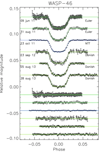
Figure 2. Phased light curves of the transits of WASP-46 b, ob-served with the Euler, NTT, and Danish telescopes, compared with the best-fitting curves given by jktebop. The date and the telescope used for each transit event are indicated close to the corresponding light curve. The residuals relative to each fit are displayed at the base of the figure in the same order as the light curves.The curves are shifted along the y axis for clarity.
of several reference stars in the FOVs, selecting those of sim-ilar brightness to the target and not showing any significant brightness variation due to intrinsic variability or instru-mental effects. For each dataset, we tried different aperture sizes for both the inner and outer rings, and the final ones that we selected (see Table 1) were those that gave the low-est scatter in the out-of-transit (OOT) region. Light curves were then obtained by performing differential photometry using the reference stars in order to correct for non-intrinsic variations of the flux of the target, which are caused by at-mospheric or air-mass changes. Also in this case we tried dif-ferent combinations of multiple comparison stars and chose those that gave the lowest scatter in the OOT region. We no-ticed that the different options gave consistent transit shapes but had a small effect on the scatter of the points in the light curves. Finally, each light curve was obtained by optimising the weights of the chosen comparison stars.
The EulerCam photomety was also extracted using rel-ative aperture photometry with the extraction being per-formed for a number of target and sky apertures, of which the best was selected based on the final lightcurve RMS. The selection of the reference stars was done iteratively,
op-Figure 3. Phased light curves of four transits of WASP-46 ob-served with GROND. Each transit was obob-served simultaneously in four optical bands. As in Figs. 1 and 2 the light curves are compared with the best-fitting curves given by jktebop, and the residuals from the fits are displayed at the bottom in the same order as the light curves.The curves are shifted along the y axis for clarity.
timizing the scatter of the full transit lightcurves based on preliminary fits of transit shapes to the data at each op-timization step. For further details, please see Lendl et al. (2012).
To properly compare the different light curves and avoid underestimation of the uncertainties assigned to each pho-tometric point, we inflated the errors by multiplying them by thepχ2
ν (defined as χν2 = Σ((xi− xbest)2/σ2)/ DOF,
Table 2. FEROS RV measurements of WASP-45. Date of observation RV errRV
BJD-2400000 km s−1 km s−1 56939.69704138 4.368 0.010 56941.64378526 4.557 0.011 56942.69196252 4.382 0.010 57037.53926492 4.650 0.010 57049.54110894 4.502 0.010
from the first fit of each light curve. We then took into ac-count the possible presence of correlated noise or systematic effects using the β approach (e.g. Gillon et al. 2006; Winn et al. 2007), with which we further enlarged the uncertainties. The NIR light curves observed with GROND were re-duced following Chen et al. (2014b), by carefully subtract-ing the dark from each image and flat-fieldsubtract-ing them, and correcting for the read-out pattern. No sky subtraction was performed since no such calibration files were available. Un-fortunately, the quality of the data was not good enough to proceed with a detailed analysis of the transits.
FEROS spectra reduction
The spectra obtained with FEROS were extracted using a new pipeline written for ´echelle spectrographs, adapted for this instrument and optimised for the subsequent RV mea-surements (Jord´an et al. 2014; Brahm et al. 2015). In brief, first a master-bias and a master-flat were constructed as the median of the frames obtained during the afternoon rou-tine calibrations. The master-bias was subtracted from the science frames in order to account for the CCD intrinsic in-homogeneities, while the master-flat was used to find and trace all 39 ´echelle orders. The spectra of the target and the calibration ThAr lamp were extracted following Marsh (1989). The science spectrum was then calibrated in wave-length using the ThAr spectrum, and a barycentric correc-tion was applied. In order to measure the RV of the star, the spectrum was cross-correlated with a binary mask cho-sen according to the spectral class of the target. For each ´
echelle order a cross correlation function (CCF) was found and the RV measured by fitting a combined one, which is obtained as a weighted sum of all the CCF, with a Gaussian. The uncertainties on the RVs were calculated using empir-ical scaling relations from the width of the CCF and the mean S/N measured around 570 nm. The RV measurements are reported in Table 2.
3 LIGHT CURVE ANALYSIS
The light curve shape of a transit (its depth and duration) directly depends on values that describe the planet and its host star (e.g. Seager & Mall´en-Ornelas 2003). In particular, by fitting the transit shape it is possible to obtain the mea-surement of the stellar and planetary relative radii, r∗= Ra∗
and rb= Rab (where a is the semi-major axis of the orbit),
the inclination of the planetary orbit with respect to the line of sight of the observer, i, and the time of the transit centre, T0.
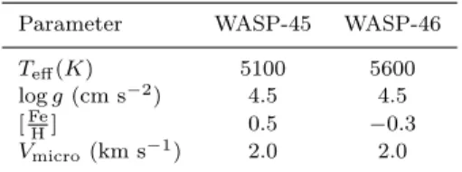
Table 3. Stellar atmospheric parameters used to calculate the LD coefficients used to model the light curves.
Parameter WASP-45 WASP-46 Teff(K) 5100 5600
log g (cm s−2) 4.5 4.5 [FeH] 0.5 −0.3 Vmicro(km s−1) 2.0 2.0
Using the jktebop1code (version 34, Southworth 2013,
and references therein), we separately fitted each light curve initially setting the fitted parameters to the values pub-lished in the discovery paper. The values for each parameter were then obtained through a Levenberg-Marquardt min-imisation, while uncertainties were estimated by running Monte Carlo and residual-permutation algorithms (South-worth 2008). The coefficients of a second order polynomial were also fitted to account for instrumental and astrophysi-cal trends possibly present in the light curves. In particular, 10 000 simulations for the Monte Carlo and Ndata-1 simula-tions for residual-permutation algorithm were run, and the larger of the two 1-σ values were adopted as the final un-certainties. The jktebop code is capable of simultaneously fitting light curves and RVs, and therefore giving also an estimation of the semi-amplitude K and systemic velocity γsys.
To properly constrain the planetary system’s quantities we took into account the effect of the star’s limb darkening (LD) while the planet is transiting the stellar disc. We ap-plied a quadratic law to describe this effect, and used the LD coefficients provided by the stellar models of Claret (2000, 2004) once the stellar atmospheric parameters were supplied (Table 3). Each light curve was firstly fitted for the linear co-efficient, while the quadratic one was perturbed during the Monte Carlo and residual-permutation algorithms in order to account for its uncertainty. Then we repeated the fitting process whilst keeping both the LD coefficients fixed.
Considering the discussion in A12, we fixed the eccen-tricity to zero for both the planetary systems. As an ex-tra check, we used the Systemic Console 2 (Meschiari et al. 2009) to fit the RVs published in the discovery paper and those we observed with FEROS, obtaining a value consis-tent with e = 0 (from the fit we obtained e = 0.041 ± 0.043 for WASP-45). All the light curves observed along with the best fit are shown in Fig.1 for WASP-45 and Figs. 2 and 3 for WASP-46.
3.1 New orbital ephemeris
From the fit of each light curve, we obtained, among the other properties, accurate values of the mid-transit times. By also taking into account the values found from the dis-covery paper A12 and those from the Exoplanet Transit Database (ETD)2 website, we refined the ephemeris values.
In particular for WASP-46 we used only those light curves from the ETD catalogue that had a data quality index better
1 The jktebop source code can be downloaded at http://
www.astro.keele.ac.uk/jkt/codes/jktebop.html
Table 4. Times of mid-transit point of WASP-45 b and their residuals. References: (1)A12; (2) ETD; (3) Euler, this work; (4) GROND, this work; (5) Danish, this work.
Time of minimum Epoch Residual Reference BJD(TDB)−2400000 (JD) 55441.27000 ± 0.00058 0 -0.00128 (1) 55782.01007 ± 0.00235 109 0.00310 (2) 55872.67006 ± 0.00030 138 -0.00011 (3) 56119.62852 ± 0.00081 217 0.00301 (2) 56172.77422 ± 0.00018 234 0.00094 (5) 56216.54008 ± 0.00029 248 0.00042 (4) g 56216.54153 ± 0.00021 248 -0.00103 (4) r 56216.54110 ± 0.00024 248 -0.00060 (4) i 56216.54001 ± 0.00025 248 0.00049 (4) z 56497.88958 ± 0.00026 338 -0.00044 (5)
Table 5. Times of mid-transit point of WASP-46 b and their residuals. References: (1) A12; (2) ETD; (3) Euler, this work; (4) NTT, this work; (5) GROND, this work; (6) Danish, this work.
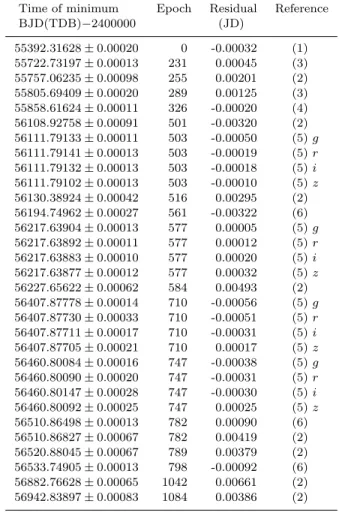
Time of minimum Epoch Residual Reference BJD(TDB)−2400000 (JD) 55392.31628 ± 0.00020 0 -0.00032 (1) 55722.73197 ± 0.00013 231 0.00045 (3) 55757.06235 ± 0.00098 255 0.00201 (2) 55805.69409 ± 0.00020 289 0.00125 (3) 55858.61624 ± 0.00011 326 -0.00020 (4) 56108.92758 ± 0.00091 501 -0.00320 (2) 56111.79133 ± 0.00011 503 -0.00050 (5) g 56111.79141 ± 0.00013 503 -0.00019 (5) r 56111.79132 ± 0.00013 503 -0.00018 (5) i 56111.79102 ± 0.00013 503 -0.00010 (5) z 56130.38924 ± 0.00042 516 0.00295 (2) 56194.74962 ± 0.00027 561 -0.00322 (6) 56217.63904 ± 0.00013 577 0.00005 (5) g 56217.63892 ± 0.00011 577 0.00012 (5) r 56217.63883 ± 0.00010 577 0.00020 (5) i 56217.63877 ± 0.00012 577 0.00032 (5) z 56227.65622 ± 0.00062 584 0.00493 (2) 56407.87778 ± 0.00014 710 -0.00056 (5) g 56407.87730 ± 0.00033 710 -0.00051 (5) r 56407.87711 ± 0.00017 710 -0.00031 (5) i 56407.87705 ± 0.00021 710 0.00017 (5) z 56460.80084 ± 0.00016 747 -0.00038 (5) g 56460.80090 ± 0.00020 747 -0.00031 (5) r 56460.80147 ± 0.00028 747 -0.00030 (5) i 56460.80092 ± 0.00025 747 0.00025 (5) z 56510.86498 ± 0.00013 782 0.00090 (6) 56510.86827 ± 0.00067 782 0.00419 (2) 56520.88045 ± 0.00067 789 0.00379 (2) 56533.74905 ± 0.00013 798 -0.00092 (6) 56882.76628 ± 0.00065 1042 0.00661 (2) 56942.83897 ± 0.00083 1084 0.00386 (2)
than 3 and whose light curve didn’t show evident deviation from a transit shape that could affect the T0 measurement.
The new values for the period and the reference time of mid-transit, T0, were obtained performing a linear fit to all
the mid-transit times versus their cycle number (see Tables 4 and 5). We obtained:
T0= BJD(TDB) 2 455 441.2687 (10) + 3.1260960 (49) E,
for WASP-45, and
T0= BJD(TDB) 2 455 392.31659 (58) + 1.43036763 (93) E.
for WASP-46, where the numbers in brackets represent the uncertainties on the last digit of the number they follow, and E is the number of orbits the planet has completed since the T0 used as reference. The presence of an additional
plane-tary companion in either of the two systems can be detected thanks to the gravitational effects that it would generate on the motion of the known bodies. Indeed, if another planet orbits the same star as WASP-45 b or WASP-46 b, it will affect their orbital motion, by periodically advancing and retarding the transit time (e.g. Holman & Murray 2005; Lis-sauer et al. 2011). Here, the fit has a χν2= 9.5 and 22.7 for
WASP-45 and WASP-46, respectively, indicating that the linear ephemeris is not a good match to the observations in both the cases. As noted in previous cases (e.g. Southworth et al. 2015), this is an indication that the measured timings have too small uncertainties rather than the presence of a co-herent TTV. The plots of the residuals, displayed in Figs. 4 and 5, do not show any evidence for systematic deviations from the predicted transit times. Indeed, by fitting the resid-uals with both a linear and sinusoidal function, we did not find any significative correlation or periodic signal. However, more precise and homogenous measurements of the timings are mandatory to robustly establish the presence of a TTV in any of the two planetary systems.
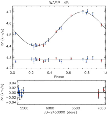
A signature of additional planetary or more massive bodies in one of the two systems can also be found by look-ing for a periodicity or a linear trend in the residual of the RV data, once the sinusoidal signal due to the known planet is removed (e.g. Butler et al. 1999; Marcy et al. 2001). Con-sidering both the data from the discovery paper and the new ones presented in this work, we studied the distribution of the RV residuals in time for WASP-45 (shown in Fig. 6 along with the best fit), but did not find any particular trend.
This is not surprising given the low probability to find a close in companion to a hot Jupiter (e.g. Mustill et al. 2015; Ford 2014; Izidoro et al. 2015).
3.2 Final photometric parameters
For both the planets, each final photometric parameter was obtained as a weighted mean of the values extracted from the fit of all the individual light curves, using the relative errors as a weight. The final uncertainties, also obtained from the weighted mean, were subsequentely rescaled according to the pχ2
ν calculated for each quantity. The results together with
their uncertainties and the relative χν2 are shown in Table 6,
in which they are compared with those from the discovery paper A12. The photometric parameters obtained from each single light curve are reported in Tables A1 and A2 in the Appendix.
For both planets, we decided to adopt the results ob-tained from the fit in which we fixed the LD coefficients for all light curves. This choice was dictated by the following reasoning. In near-grazing transits, only the region near the limb of the star is transited, so there is very little informa-tion on its LD (Howarth 2011; M¨uller et al. 2013). As the impact parameters of the systems are high (b = 0.87 for WASP-45 and b = 0.71 for WASP-46) and thus the transits
Figure 4. Plot of the residuals of the timing of mid-transit of WASP-45 versus a linear ephemeris. The different colours of the points refer to the value from the discovery paper (blue), values obtained from the ETD catalogue (green), and our data (red).
Figure 5. Plot of the residuals of the timing of mid-transit of WASP-46 versus a linear ephemeris. The different colours of the points refer to the value from the discovery paper (blue), values obtained from the ETD catalogue (green), and our data (red).
Figure 6. Upper panel : RV measurements with the best fit obtained from jktebop; residuals are displayed at the bottom. Lower panel : residuals of the best fit displayed as a function of the days when the spectra were observed. In both the panels blue points refer to the data from the discovery paper A12, whilst the red ones are those observed with FEROS.
are nearly-grazing, we decided to not fit for the LD coef-ficients in order to avoid biasing the results. However, we checked that the results, obtained either fixing or fitting for the LD coefficients, were compatible with each other. We assigned to the parameters of each light curve a 1-σ uncer-tainty, estimated by Monte Carlo simulations, because these values were systematically higher than those obtained with the residual-permutation algorithm.
4 PHYSICAL PROPERTIES OF WASP-45 AND
WASP-46
Using the results obtained from the photometry (Table 6) and taking into account the spectroscopic results from the discovery paper, we redetermined the main physical param-eters that characterise the two planetary systems. Follow-ing the methodology described in Southworth (2010), the missing information such as the age of the system and the planetary velocity semi-amplitude were iteratively interpo-lated using stellar evolutionary model predictions until the best fit to the photometric and spectroscopic parameters was reached. This was done for a sequence of ages separated by 0.1 Gyr and covering the full main sequence lifetimes of the stars. We independently repeated the interpolation us-ing different stellar models (Girardi et al. 2000; Claret 2004; Demarque 2004; Pietrinferni et al. 2004; VandenBerg 2006; Dotter 2008); for a complete list see Southworth 2010), and the final values were obtained as a weighted mean. In the final results presented in Tables 7 and 8, the first uncer-tainty is a statistical one, which is derived by propagating
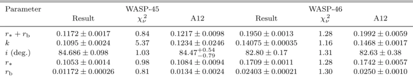
Table 6. Photometric properties of the WASP-45 and WASP-46 systems derived by fitting the light curves with jktebop, and taking the weighted mean of the single values obtained from each transit. The values from the discovery paper A12 are shown for comparison. k is the ratio of the planetary and stellar radii, i the orbital inclination, r∗and rbthe stellar and planetary relative radii respectively.
Parameter WASP-45 WASP-46
Result χ2
ν A12 Result χν2 A12
r∗+ rb 0.1172 ± 0.0017 0.84 0.1217 ± 0.0098 0.1950 ± 0.0013 1.28 0.1992 ± 0.0059
k 0.1095 ± 0.0024 5.37 0.1234 ± 0.0246 0.14075 ± 0.00035 1.16 0.1468 ± 0.0017 i (deg.) 84.686 ± 0.098 1.03 84.47+0.54−0.79 82.80 ± 0.17 1.31 82.63 ± 0.38 r∗ 0.1053 ± 0.0014 0.98 0.1084 ± 0.0094 0.1709 ± 0.0011 1.28 0.1742 ± 0.0057
rb 0.01172 ± 0.00026 0.81 0.0134 ± 0.0024 0.02403 ± 0.00021 1.30 0.0250 ± 0.0010
Table 7. Final results for the physical parameters of WASP-45 obtained in this work compared to those of the discovery paper. The mass M , radius R, surface gravity g and mean density ρ for the star and the planet are displayed; as well as the equilib-rium temperature of the planet, the Safronov number Θ, the semi major axis a and the age of the system.(a)This is the
gyrochrono-logical age measured in A12. The same authors also obtained a value for the stellar age from lithium abundance measurements, finding that the star is at least a few Gyr old.
This work A12 M∗(M ) 0.904 ± 0.066 ± 0.010 0.909 ± 0.060 R∗(R ) 0.917 ± 0.024 ± 0.003 0.945+0.087−0.071 log g∗(cgs) 4.470 ± 0.014 ± 0.002 4.445+0.065−0.075 ρ∗(ρ ) 1.174 ± 0.047 1.08+0.27−0.24 Mb(Mjup) 1.002 ± 0.062 ± 0.007 1.007 ± 0.053 Rb(Rjup) 0.992 ± 0.038 ± 0.004 1.16+0.28−0.14 gb(ms−2) 25.2 ± 1.3 17.0+4.9−6.0 ρb(ρjup) 0.959 ± 0.077 ± 0.003 0.64 ± 0.30 Teq(K) 1170 ± 24 1198 ± 69 Θ 0.0903 ± 0.0044 ± 0.0003 − a (AU) 0.0405 ± 0.0010 ± 0.0001 0.04054 ± 0.00090 Age (Gyr) 7.2+5.8 +6.8−9.0 −1.2 1.4 +2.0 −1.0a
the uncertainties of the input parameters, while the second is a systematic uncertainty, which takes into account the dif-ferences in the predictions coming from the different stellar models used. The final values for the ages of the two system are not well constrained. The uncertainty that most affects the precision on these measurements is the large errorbars on Teff (from A12 Teff = 5140 ± 200 and Teff = 5620 ± 160
for WASP-45 and WASP-46 respectively). Moreover, we no-ticed that for metallicity different to solar, the discrepancies between the different stellar models increase and therefore the systematic errorbar on the age estimation swells.
5 RADIUS VS WAVELENGTH VARIATION
During a transit event, a fraction of the light coming from the host star passes through the atmosphere of the planet and, according to the atmospheric composition and opac-ity, it can be scattered or absorbed at specific wavelengths (Seager & Sasselov 2000). Similarly to transmission spec-troscopy, by observing a planetary transit at different bands simultaneously, it is then possible to look for variations in the value of the planet’s radius measured in each band, and
Table 8. Final results for the physical parameters of WASP-46 obtained in this work compared to those of the discovery paper. See Table. 7 for the description of the parameters listed. This is the gyrochronological age measured in A12.(a)The same authors
also obtained a value for the stellar age from lithium abundance measurements, finding that the star is at least a few Gyr old.
This work A12 M∗(M ) 0.828 ± 0.067 ± 0.036 0.956 ± 0.034 R∗(R ) 0.858 ± 0.024 ± 0.013 0.917 ± 0.028 log g∗(cgs) 4.489 ± 0.013 ± 0.006 4.493 ± 0.023 ρ∗(ρ ) 1.310 ± 0.025 1.24 ± 0.10 Mb(Mjup) 1.91 ± 0.11 ± 0.06 2.101 ± 0.073 Rb(Rjup) 1.174 ± 0.033 ± 0.017 1.310 ± 0.051 gb(ms−2) 34.3 ± 1.1 28.0+2.2−2.0 ρb(ρjup) 1.103 ± 0.050 ± 0.016 0.94 ± 0.11 Teq(K) 1636 ± 44 1654 ± 50 Θ 0.0916 ± 0.0035 ± 0.0014 − a (AU) 0.02335 ± 0.00063 ± 0.000340.02448 ± 0.00028 Age (Gyr) 9.6+3.4 +1.4−4.2 −3.5 1.4+0.4−0.6(a)
thus probe the composition of its atmosphere (e.g. South-worth et al. 2012; Mancini et al. 2013a; Narita et al. 2013). To pursue this goal, we phased and binned all the light curves observed with the same instrument and filter, and performed once again a fit with jktebop. Following South-worth et al. (2012), we fixed all the parameters to the final values previously obtained (see Tables 7 and 8) and fitted just for the planetary and stellar radii ratio k. In this way, we removed sources of uncertainty common to all datasets, maximising the relative precision of the planet/star radius ratio measurements as a function of wavelength. In order to have a set of data as homogeneous as possible, we preferred to use the light curves obtained with the same reduction pipeline and, thus, we excluded the light curves from the Euler telescope from this analysis.
The values of k that we obtained at different passbands are reported in Table 9 and illustrated in Figs. 7 and 8 for WASP-45 and WASP-46, respectively. In these figures, for comparison, we also show the expected values of the planetary radius in function of wavelength, obtained from synthetic spectra constructed from model planetary atmo-spheres by Fortney et al. (2010), using different molecular compositions. The models were estimated for a Jupiter-mass planet with a surface gravity of gp= 25 m s−2, a base radius
of 1.25 RJup at 10 bar, and Teq = 1250 K and 1750 K for
WASP-45 b and WASP-46 b, respectively. The model dis-played with a red line in Fig. 8 was run in an isothermal
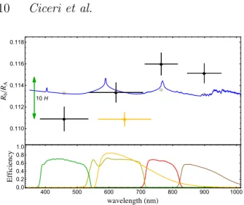
Figure 7. Variation of the radius of WASP-45 b, in terms of planet/star radius ratio, with wavelength. The black points are from the transit observed with GROND, and the yellow point is the weighted-mean results coming from the two transits observed with the Danish telescope. The vertical bars represent the uncer-tainties in the measurements and the horizontal bars show the FWHM transmission of the passbands used. The observational points are compared to a synthetic spectrum for a Jupiter-mass planet with a surface gravity of gp= 25 m s−2, and Teq= 1250 K.
An offset was applied to the model to provide the best fit to our radius measurements. Transmission curves of the filters used are shown in the bottom panel. On the left of the plot the size of ten atmospheric pressure scale heights (10 H) is shown. The small coloured squares represent band-averaged model radii over the bandpasses used in the observations.
case taking into account chemical equilibrium and the pres-ence of strong absorbers, such as TiO and VO. The models displayed with blue lines in Figs. 7 and 8 were obtained omitting the presence of the metal oxides.
Looking at the distribution of the experimental points in the two figures, we do not see the telltale increase of the radius at the shortest wavelengths (e.g. see Lecavelier Des Etangs et al. 2008), and therefore we do not expect a strong Rayleigh scattering in the atmosphere. However by study-ing our data points quantitatively we can not exclude any hypothesis. By performing a Monte Carlo simulation, we obtained that our data points are consistent within 3σ to a slope with a maximum inclination of m = −1.40 × 10⁻⁵for WASP-45 b and m = −1.17 × 10⁻⁵ for WASP-46 b (where with m we indicate the slope coefficient of the best linear fit). Fitting with a straight line the predictions given at short wavelengths by a model with the Rayleigh scattering en-hanced by a factor of 1000, we obtained slope coefficients lower that the ones just mentioned (the slope coefficient is m = −2.2 × 10⁻⁶, and m = −3.3 × 10⁻⁶ for WASP-45 and WASP-46, respectively). Although pointing in the direction of no strong Rayleigh scattering, our data are not sufficient to completely rule out this scenario. More data points are needed to make stronger statements regarding this matter.
For the case of WASP-45 b, for which we have only one transit observed with GROND, it is possible to note a radius variation between the g0 and i0 bands at 2σ, correspond-ing to roughly 12H pressure scale heights (where the
atmo-Figure 8. Variation of the radius of WASP-46 b, in terms of planet/star radius ratio, with wavelength. The black points are from the transit observed with GROND, the green point is that obtained with the NTT, and the yellow point is the weighted-mean result coming from the three transits observed with the Danish telescope. The vertical bars represent the uncertainties in the measurements and the horizontal bars show the FWHM transmission of the passbands used. The observational points are compared to two synthetic spectra for a Jupiter-mass planet with a surface gravity of gp= 25 m s−2, and Teq= 1750 K. The
syn-thetic spectrum in blue does not include TiO and VO opacity, while the spectrum in red does, based on equilibrium chemistry. An offset was applied to the models to provide the best fit to our radius measurements. Transmission curves of the filters used are shown in the bottom panel. On the left of the plot the size of four atmospheric pressure scale heights (4 H) is shown. The small coloured squares represent band-averaged model radii over the bandpasses used in the observations.
Table 9. Values of k for each of the light curves as plotted in Figs. 7 and 8. Passband Central FWHM k wavelength (nm) (nm) WASP-45: GROND g0 477.0 137.9 0.11090 ± 0.00111 GROND r0 623.1 138.2 0.11335 ± 0.00090 Bessel R 648.9 164.7 0.11088 ± 0.00062 Gunn r 664.1 85.0 0.10821 ± 0.00099 GROND i0 762.5 153.5 0.11598 ± 0.00103 GROND z0 913.4 137.0 0.11513 ± 0.00089 WASP-46: GROND g0 477.0 137.9 0.13950 ± 0.00031 Gunn g 516.9 77.6 0.13961 ± 0.00047 GROND r0 623.1 138.2 0.13943 ± 0.00032 Bessel R 648.9 164.7 0.13990 ± 0.00043 Gunn r 664.1 85.0 0.13815 ± 0.00113 GROND i0 762.5 153.5 0.13871 ± 0.00039 GROND z0 913.4 137.0 0.14059 ± 0.00042
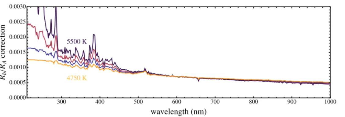
300 400 500 600 700 800 900 1000 0.0000 0.0005 0.0010 0.0015 0.0020 0.0025 0.0030 wavelength HnmL Rb RA correction 5500 K 4750 K
Figure 9. The effect of the presence of unocculted starspot on the surface of the star on the transmission spectrum, considering a 1 per cent flux drop at 600nm. The stellar temperature adopted is Teff = 5600 K, and the spots coverage is modelled using a grid of stellar
atmospheric models of different temperature ranging from 4750 (yellow line) to 5500 (purple line), with steps of 250 K.
spheric pressure scale height is H = k Teq/µ g, with k being
the Boltzmann constant, Teqthe planetary atmosphere
tem-perature, µ the mean molecular weight and g the planet’s surface gravity). In the case of WASP-46 b, for which we ob-served four transits with GROND, we noticed a small vari-ation of ∼ 4 H between the i0 and z0 bands but at only 1.5σ. These detections are too small to be significant – both planets are not well suited to transmission photometry or spectroscopy due to their large impact parameters and high surface gravities.
As stated in A12, the lightcurve of WASP-46 shows a rotational modulation, which is symptomatic of stellar activ-ity. The presence of star spots on the stellar surface, and in general stellar activity, can produce variations in the transit depth when it is measured at different epochs. In particular, we expected that such a variation is stronger at bluer wave-lengths and affecting more the lightcurves obtained through the g0band, whereas it is negligible in the i and z bands (e.g., Sing et al. 2011; Mancini et al. 2014). Correcting for this ef-fect, would slightly shift the data point relative to the bluer bands, towards the bottom of Fig. 7. Anyway, since the stel-lar activity is not particustel-larly high, the expected variation in the transit depth is small and within our errorbars (Fig. 9 shows the effect of the presence of starspots, at different temperatures, on the transit depth with wavelength. The stellar model used to produce the curves are the ATLAS9 by Castelli & Kurucz 2004).
6 SUMMARY AND CONCLUSIONS
We have presented new multi-band photometric light curves of transit events of the hot-Jupiter planets WASP-45 b and WASP-46 b, and new RV measurements of WASP-45. We used these new datasets to refine the orbital and physical parameters that characterise the architecture of the WASP-45 and WASP-46 planetary systems. Moreover, we used the light curves observed through several optical passbands to probe the atmosphere of the two planets. Our conclusions are as follows:
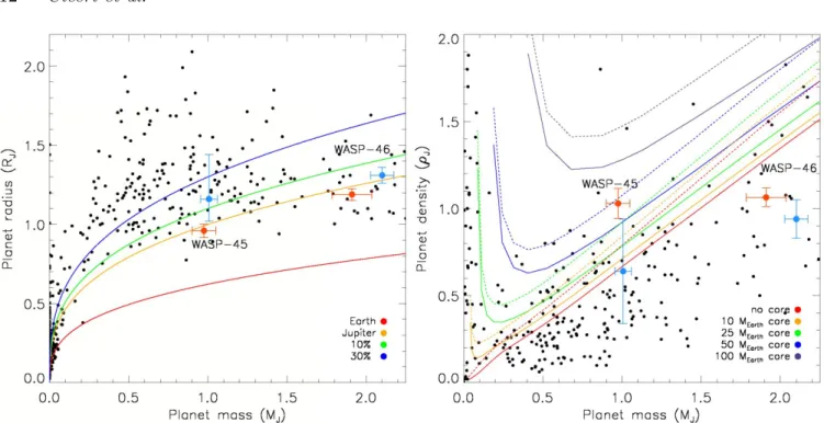
• The radius of WASP-45 b is now much better con-strained, with a precision better by almost one order of magnitude with respect to that of A12. We found that WASP-46 b has a slightly lower radius (1.189 ± 0.037 RJup)
compared to the previous estimation (1.310 ± 0.051 RJup).
The left panel of Fig. 10 shows the change in position in the planet mass-radius diagram for both WASP-45 b and WASP-46 b.
• Based on our estimates, both planets have a larger density than previously thought (see the right panel of Fig. 10). In particular, WASP-45 b appears to be one of the densest planets in its mass regime (there are only 3 other planets with masses between 0.7 and 1.3MJup that
have similar or higher density), suggesting the presence of a heavy-element core of roughly 50 M⊕(Fortney et al. 2007).
• By studying the transit times and the RV residuals we did not find any hint for the presence of any additional planetary companion in either of the two planetary systems. However more spectroscopic and photometric data are nec-essary to claim a lack of other planetary companions, at any mass and separation, in these two systems. In particular a higher temporal cadence for the photometric observations could allow to detect the signature of smaller inner planets, while RV measurements obtained at different epochs separated by several months/years could provide information on the presence of outer long period planets.
• Looking at the radius variation in terms of wave-length, we estimated the upper limit of the slope allowed by our data within 3σ. The slope of the best linear fit are m = −1.40 × 10⁻⁵ and m = −1.17 × 10⁻⁵ for WASP-45 b and WASP-46 b respectively. Comparing these values to the slope obtained from a model with 1000 times enhancement of Rayleigh scattering we found that we can not exclude with a high statistical significance the presence of strong Rayleigh scattering in the atmospheres of both planets.
The data of one transit of WASP-45 b, observed simul-taneously in four optical bands with GROND, indicate a planetary radius variation of more than 10 H between the g0 and the i0bands, but at only a ∼ 2σ significance level. Such a variation is rather high for that expected for a planet with a temperature below 1200 K, and would require the presence of strong absorbers between 800 and 900 nm. More observa-tions are requested to verify this possible scenario.
In the case of WASP-46 b, by joining the GROND multi-colour data of four transit events, we detected a very small radius variation, roughly 4 H, between the i0 and z0 bands, but at only a 1.5σ significance level. This variation can be
Figure 10. Left : the mass versus radius diagram of the known transiting planets. The values for WASP-45 b and WASP-46 b obtained in this work are displayed in orange, and for comparison we also show in light blue the measurements reported in the discovery paper. The coloured curves represent the iso-density lines for planets with the density of Earth and Jupiter, and with a density equal to a Jupiter-like planet with a radius inflated by 10% and 30%. Right : the mass versus density diagram of the known transiting planets. As in the left panel, the values obtained for WASP-45 and WASP-46 are highlighted in colour. The superimposed lines represent the expected radius of the planet having an inner core of 0, 10, 25, 50 and 100 Earth masses, and calculated for 10 Gyr old planets at 0.02 au, solid lines, and 0.045 au, dashed lines (Fortney et al. 2007).
explained by supposing the absence of potassium at 770 nm and a significant amount of water vapour around 920 nm.
ACKNOWLEDGMENTS
We acknowledge the use of the NASA Astrophysics Data System; the SIMBAD database operated at CDS, Stras-bourg, France; and the arXiv scientific paper preprint service operated by Cornell University. This work was supported by KASI (Korea Astronomy and Space Science Institute) grants 2012-1-410-02 and 2013-9-400-00. ASB acknowledges support from the European Union Seventh Framework Pro-gramme (FP7/2007-2013) under grant agreement number 313014 (ETAEARTH). TCH acknowledges financial support from the Korea Research Council for Fundamental Science and Technology (KRCF) through the Young Research Scien-tist Fellowship Program. YD, AE, JSurdej and OW acknowl-edge support from the Communaut´e fran¸caise de Belgique – Actions de recherche concert´ees – Acad´emie Wallonie-Europe. SHG and XBW would like to thank the financial support from National Natural Science Foundation of China through grants Nos. 10873031 and 11473066. SC thanks G-D. Marleau for useful discussion and comments, the staff and astronomers observing at the ESO La Silla observatory during January and February 2015 for the great, friendly and scientifically stimulating environment.
REFERENCES
Alonso, R., Brown, T. M., Torres, G., et al. 2004, ApJ, 613, 153
Alsubai, K. A., Parley, N. R., Bramich, D. M., et al. 2013, AcA, 63, 465
Anderson, D. R., Collier Cameron, A., Gillon, M., et al. 2012,MNRAS, 422, 1988
Bakos, G. ´A., Noyes, R. W., Kov´acs, G., et al. 2004,PASP, 116, 266
Bakos, G. ´A., Csubry, Z., Penev, K., et al. 2013,PASP, 125, 154
Baraffe, I., Chabrier, G., Fortney, J., 2014, Protostar and Planet VI conference proceedings, 763
Barge, P., Baglin, A., Auvergne, M., et al. 2008, A&A, 482, L17
Baruteau, C., Crida, A., Paardekooper, et al. 2014, Proto-star and Planet VI conference proceedings, 667
Borucki, W. J., Koch, D., Basri, G., et al. 2011, ApJ, 728, 20
Brahm, R., et al. 2015, in prep.
Butler, R., Marcy, G. W., Fischer, D. A., et al. 1999, ApJ, 526, 916
Castelli, F., & Kurucz, R. L., 2004, (arXiv:sstro-ph/0405087)
Charbonneau, D., Brown, T. M., Noyes, R. W., Gilliland, R. L., 2002, ApJ, 568, 377
Charbonneau, D., Berta, Z. K., Irwin, J., et al. 2009, Na-ture, 462, 891
Chen, G., van Boekel, R., Wang, H., et al. 2014, A&A, 567, A8
Chen, G., van Boekel, R., Wang, H., et al. 2014, A&A, 563, A40
Claret, A., 2000, A&A, 363, 1081 Claret, A., 2004, A&A, 428, 1001
Demarque P., Woo J.-H., Kim Y.-C., Yi S. K., 2004, ApJS, 155, 667
Dotter A., Chaboyer B., Jevremovic D., et al., 2008, ApJS, 178, 89
Ford, E. B., 2014, PNAS, 111, 12616
Fortney, J. J., Marley, M. S. & Barnes, J. W., 2007, ApJ, 659, 1661
Fortney, J. J., Shabram, M., Showman, A. P., et al. 2010, ApJ, 709, 1396
Gillon, M., Pont, F., Moutou, C., et al. 2006, A&A, 459, 249
Girardi, L., Bressan, A., Bertelli, G., 2000, A&AS, 141, 371 Greiner, J., Bornemann, W., Clemens, C., et al. 2008,
PASP, 120, 405
Hellier, C., Anderson, D.R., Collier Cameron, A., et al. 2011, PASP, 120, 405
Holman, M. J. & Murray, N. W. 2005, Science, 307, 1288 Howarth, I. D., 2011, MNRAS, 418, 1165
Izidoro, A., Raymond, S. N., Morbidelli, A., et al. 2015, ApJL, 800, 22
Jones, M. I., Jenkins, J. S., Rojo, P., et al. 2015, A&A, 573, 3
Jord´an, A., Brahm, R., Bakos, G. ´A., et al. 2014, AJ, 148, 29
Kley, W., & Nelson, R. P., 2012, A&A Rev, 50, 211 Kreidberg, L., Bean, J. L., D´esert, J.-M., 2014, Nature, 505,
66
Lendl, M., Anderson, D.R., Collier Cameron, A., et al. 2012, A&A, 544, 72
Lendl, M., Gillon, M., Queloz, D., et al. 2013, A&A, 552, 2
Lendl, M., Triaud, A.H.M.J., Anderson, D.R., et al. 2014, A&A, 568, 81
Lecavelier Des Etangs, A., Pont, F., Vidal-Madjar, A., Sing, D., 2008, A&A, 481, 83L
Lissauer, J. J., Fabrycky, D.C., Ford, E. B., et al. 2011, Nature, 470, 53
McCullough, P. R., Stys, J. E., Valenti, J. A., et al. 2005, PASP, 117, 783
Mancini, L., Southworth, J., Ciceri, S., et al. 2013a, A&A, 551, A11
Mancini, L., Ciceri, S., Chen, G., et al. 2013b, MNRAS, 436, 2
Mancini, L., Southworth, J., Ciceri, S., et al. 2014, MN-RAS, 443, 2391
Marcy, G. W., Butler, R. P., Fischer, D., et al. (2001), ApJ, 556, 296
Marsh, T. R. (1989), PASP, 101, 1032
Meschiari, S., Wolf, A. S., Rivera, E., et al. 2009, PASP, 121, 1016
M¨uller, H. M., Huber, K. F., Czesla, S., et al. 2013, A&A, 560, 112
Mustill, A. J., Davies, M. B., Johansen, A., 2015, submitted to ApJ, (arXiv:1502.06971)
Narita, N., Nagayama, T., Suenaga, T., et al. 2013, PASJ, 65, 27
Penev, K., Bakos, G. ´A., Bayliss, D., et al. 2013, AJ, 145, 5
Pepper, J., Pogge, R. W., DePoy, D. L., et al. 2007, PASP, 119, 923
Pietrinferni A., Cassisi S., Salaris M., Castelli F., 2004, ApJ, 612, 168
Pollacco, D. L., Skillen, I., Collier Cameron, A., et al. 2006, PASP, 118, 1407
Richardson, L. J., Deming, D., Wiedemann, G., et al. 2003, ApJ, 584, 1053
Seager, S. & Sasselov, D. D., 2000, ApJ, 537, 916 Seager, S. & Mall´en-Ornelas, G., 2003, ApJ, 585, 1038 Sing, D.K., Pont, F., Aigrain, S., et al. 2011, MNRAS, 416,
1443
Southworth, J. 2008, MNRAS, 386, 1644 Southworth, J. 2010, MNRAS, 408, 1689 Southworth, J. 2013, A&A, 557, A119
Southworth, J., Hinse, T. C., Jørgensen, U.G., et al. 2009, MNRAS, 396, 1023
Southworth, J., Mancini, L., Maxted, P. F. L., et al. 2012, MNRAS, 422, 3099
Southworth, J., Hinse, T. C., Burgdorf, M., et al. 2014, MNRAS, 444, 776
Southworth, J., Mancini, L., Ciceri, S., et al.2015, MNRAS, 447, 711
Stetson, P. B., 1987, PASP, 99, 191
VandenBerg D. A., Bergbusch P. A., Dowler P. D., 2006, ApJS, 162, 375
Winn, J. N., Holman, M. J., Bakos, G. ´A., et al. 2007, AJ,134, 1707
APPENDIX A: PHOTOMETRIC PARAMETERS In the two tables in this appendix are presented the photo-metric results obtained with jktebop from the fit of each light curve presented in the paper.
This paper has been typeset from a TEX/ LATEX file prepared
Source rA+ rb k i (deg.) rA rb Eul 1.2m 0.1218 ± 0.0044 0.1018 ± 0.0018 84.3258 ± 0.2408 0.11052 ± 0.0039 0.011255 ± 0.00053 Dan 1.54m (transit #1) 0.1188 ± 0.0032 0.1130 ± 0.0022 84.6423 ± 0.1809 0.10671 ± 0.0027 0.012061 ± 0.00049 MPG 2.2m (transit g) 0.1165 ± 0.0057 0.1155 ± 0.0063 84.7024 ± 0.3381 0.10444 ± 0.0046 0.012060 ± 0.00116 MPG 2.2m (transit r) 0.1140 ± 0.0036 0.1128 ± 0.0022 84.9141 ± 0.2079 0.10245 ± 0.0030 0.011558 ± 0.00054 MPG 2.2m (transit i) 0.1181 ± 0.0061 0.1234 ± 0.0089 84.6154 ± 0.3761 0.10516 ± 0.0046 0.012979 ± 0.00149 MPG 2.2m (transit z) 0.1198 ± 0.0046 0.1176 ± 0.0035 84.5609 ± 0.2778 0.10719 ± 0.0038 0.012601 ± 0.00079 Dan 1.54m (transit #2) 0.1076 ± 0.0060 0.1097 ± 0.0035 85.2537 ± 0.3657 0.09699 ± 0.0051 0.010640 ± 0.00088 Final results 0.1172 ± 0.0017 0.1095 ± 0.0024 84.686 ± 0.098 0.1053 ± 0.0014 0.01172 ± 0.00026 Anderson et al. (2012) 0.1217 ± 0.0098 0.1234 ± 0.0246 84.47+0.54−0.79 0.1084 ± 0.0094 0.0134 ± 0.0024
Table A1. Photometric properties of the WASP-45 system derived by fitting the light curves with jktebop. In bold are highlighted the final parameters obtained as weighted mean. The values from the discovery paper are also shown for comparison.
Source rA+ rb k i (deg.) rA rb Eul 1.2m (transit #1) 0.1964 ± 0.0190 0.13551 ± 0.00585 82.90 ± 1.31 0.1730 ± 0.0160 0.02344 ± 0.00302 Eul 1.2m (transit #2) 0.1857 ± 0.0099 0.14025 ± 0.00296 83.51 ± 0.70 0.1629 ± 0.0084 0.02284 ± 0.00158 NTT 3.58m 0.1979 ± 0.0044 0.14123 ± 0.00139 82.84 ± 0.30 0.1734 ± 0.0036 0.02449 ± 0.00074 MPG 2.2m (transit #1 g) 0.1996 ± 0.0041 0.14226 ± 0.00127 82.72 ± 0.27 0.1747 ± 0.0034 0.02485 ± 0.00068 MPG 2.2m (transit #1 r) 0.1997 ± 0.0046 0.14229 ± 0.00115 82.77 ± 0.31 0.1748 ± 0.0039 0.02487 ± 0.00072 MPG 2.2m (transit #1 i) 0.1938 ± 0.0042 0.13991 ± 0.00102 83.05 ± 0.30 0.1700 ± 0.0035 0.02379 ± 0.00063 MPG 2.2m (transit #1 z) 0.1925 ± 0.0069 0.14051 ± 0.00119 83.34 ± 0.49 0.1688 ± 0.0059 0.02372 ± 0.00100 Dan 1.54m (transit #1) 0.1901 ± 0.0095 0.14291 ± 0.00310 83.40 ± 0.69 0.1664 ± 0.0080 0.02378 ± 0.00157 MPG 2.2m (transit #2 g) 0.1971 ± 0.0048 0.14185 ± 0.00162 82.85 ± 0.33 0.1726 ± 0.0040 0.02449 ± 0.00082 MPG 2.2m (transit #2 r) 0.1902 ± 0.0037 0.13955 ± 0.00108 83.25 ± 0.25 0.1669 ± 0.0031 0.02329 ± 0.00059 MPG 2.2m (transit #2 i) 0.1968 ± 0.0042 0.14120 ± 0.00117 82.93 ± 0.29 0.1725 ± 0.0036 0.02435 ± 0.00066 MPG 2.2m (transit #2 z) 0.1953 ± 0.0041 0.14135 ± 0.00108 82.96 ± 0.28 0.1711 ± 0.0035 0.02418 ± 0.00064 MPG 2.2m (transit #3 g) 0.1805 ± 0.0103 0.13800 ± 0.00288 84.14 ± 0.80 0.1586 ± 0.0087 0.02189 ± 0.00163 MPG 2.2m (transit #3 r) 0.2067 ± 0.0053 0.14525 ± 0.00169 82.25 ± 0.33 0.1805 ± 0.0044 0.02621 ± 0.00091 MPG 2.2m (transit #3 i) 0.1562 ± 0.0149 0.13543 ± 0.00370 86.30 ± 1.69 0.1376 ± 0.0127 0.01863 ± 0.00213 MPG 2.2m (transit #3 z) 0.1723 ± 0.0093 0.13828 ± 0.00177 84.72 ± 0.76 0.1514 ± 0.0080 0.02093 ± 0.00130 MPG 2.2m (transit #4 g) 0.1971 ± 0.0061 0.13918 ± 0.00209 82.91 ± 0.41 0.1730 ± 0.0051 0.02408 ± 0.00103 MPG 2.2m (transit #4 r) 0.1958 ± 0.0149 0.14121 ± 0.00334 82.79 ± 1.01 0.1716 ± 0.0126 0.02423 ± 0.00231 MPG 2.2m (transit #4 i) 0.1789 ± 0.0113 0.13713 ± 0.00217 84.03 ± 0.82 0.1574 ± 0.0097 0.02158 ± 0.00161 MPG 2.2m (transit #4 z) 0.1945 ± 0.0090 0.14015 ± 0.00298 83.30 ± 0.69 0.1706 ± 0.0075 0.02391 ± 0.00149 Dan 1.54m (transit #2) 0.1959 ± 0.0046 0.14088 ± 0.00153 82.98 ± 0.31 0.1717 ± 0.0038 0.02419 ± 0.00076 Dan 1.54m (transit #3) 0.1930 ± 0.0049 0.14039 ± 0.00136 83.09 ± 0.34 0.1692 ± 0.0042 0.02376 ± 0.00078 Final results 0.1950 ± 0.0013 0.14075 ± 0.00035 82.80 ± 0.17 0.1709 ± 0.0011 0.02403 ± 0.00021 Anderson et al. (2012) 0.1992 ± 0.0059 0.1468 ± 0.0017 82.63 ± 0.38 0.1742 ± 0.0057 0.0250 ± 0.0010 Table A2. Photometric properties of the WASP-46 system derived by fitting the light curves with jktebop. In bold are highlighted the final parameters obtained as weighted mean. The values from the discovery paper are also shown for comparison.