Application of silicon-based camera for measurement of non-homogeneous thermal field on realistic specimen surface

HAL Id: hal-02131375

https://hal.archives-ouvertes.fr/hal-02131375

Submitted on 16 May 2019

HAL is a multi-disciplinary open access archive for the deposit and dissemination of sci-entific research documents, whether they are pub-lished or not. The documents may come from teaching and research institutions in France or abroad, or from public or private research centers.

L’archive ouverte pluridisciplinaire HAL, est destinée au dépôt et à la diffusion de documents scientifiques de niveau recherche, publiés ou non, émanant des établissements d’enseignement et de recherche français ou étrangers, des laboratoires publics ou privés.

Application of silicon-based camera for measurement of

non-homogeneous thermal field on realistic specimen

surface

Chao Zhang, Jérémy Marty, Anne Maynadier, Philippe Chaudet, Julien

Réthoré, Marie-Christine Baietto

To cite this version:

Chao Zhang, Jérémy Marty, Anne Maynadier, Philippe Chaudet, Julien Réthoré, et al.. Ap-plication of silicon-based camera for measurement of non-homogeneous thermal field on real-istic specimen surface. Applied Thermal Engineering, Elsevier, 2019, 149, pp.1186 - 1191. �10.1016/j.applthermaleng.2018.12.114�. �hal-02131375�

1

Application of silicon-based camera for measurement of

non-homogeneous thermal field on realistic specimen surface

C. Zhang a,*, J. Marty a,b, A. Maynadier c, P. Chaudet a, J. Réthoré d, M.C. Baietto a a. Department of Mechanical Engineering, LaMCos, Université de Lyon/INSA Lyon/UMR

CNRS 5259, 20 Avenue des Sciences, F-69621 Villeurbanne Cedex, France. b. ESTA LAB, 3 Rue du Dr Frery, F-90000 Belfort, France

c. Université de Bourgogne Franche-Comté, FEMTO-ST Institute, Chemin de L'épitaphe, 25000 Besançon, France

d. GeM, Ecole Centrale de Nantes/Université de Nantes/UMR CNRS 6183, 1 rue de la Noë, BP 92101, F-44321 Nantes, France

* Corresponding email: chao.zhang@insa-lyon.fr

Abstract

The high-cost low-resolution infrared cameras operating in middle infrared spectral ranges are widely used to detect the thermal fields. In this study, a low-cost high-resolution silicon-based sensor camera operating in near infrared spectral ranges is used to perform the observation of the thermal fields on the realistic specimen surface. In near-infrared spectral ranges, a small temperature variation led to a large modification in the sensor illumination, inducing acquired images with over saturation or poor dynamic range of gray levels. To address this problem, an algorithm was proposed to precisely adjust the exposure time to acquire images with constant gray level whatever the temperature evolution is, and then used in heating experiment of a steel specimen. Results showed that images with constant gray level could be acquired during the experiment. A special radiometric model was used to perform near-infrared thermography. Based on this radiometric model, the thermal fields on steel specimen surface were successfully reconstructed without measuring surface emissivity.

2

Keywords: Silicon-based camera; Realistic application; Near-infrared thermography; Thermal

fields.

1. Introduction

Temperature is a very important physical quantity. For temperature measurement, many techniques are available, e.g., thermocouple [1, 2], thermistor [3], resistance temperature detector [4], and infrared thermography [5-8], etc. As an advanced measurement technology, infrared thermography can transform the thermal energy emitted by objects into an electronic video signal [9-12]. This technique possesses several advantages: (1) contact and non-invasive; (2) full field measurement; (3) no disturbance of the target surface to be measured; (4) high-speed response; (5) possibility to measure the target objects which can be small, fragile, dangerous, and so on.

The traditional infrared cameras operating in middle infrared spectral ranges (3-12 μm) have also some disadvantages. Firstly, the disturbance radiation from the surrounding objects to the target object is necessary to be measured, but the corresponding corrections are difficult because it depends on the surface states of objects; Secondly, most of time infrared thermography required a uniform surface with homogeneous and even constant emissivity. However, for most of natural or artificial objects, their surfaces are non-homogeneous, thus these measurements are difficult for infrared thermography. To address these issues, it is effective to operate in lower spectral ranges (near infrared spectral ranges). The rapid development of silicon-based cameras makes the temperature measurement in near infrared spectral ranges possible [13-16]. Silicon-based cameras are not only operating in the visible spectral ranges (0.4-0.7 μm), but also operating in near infrared spectral ranges (0.7-1.1 μm) [17, 18]. Thus, they can be used to measure thermal fields. Teyssieux et al. [19-21] indicated that the disturbance radiation from surrounding objects is slight and can be negligible in near infrared spectral range, while the disturbance radiation from surrounding objects is obvious in

3

middle infrared spectral range. Moreover, both infrared camera and silicon-based camera were used to measure temperature distribution of the object surface with non-homogeneous emissivity by Rotrou et al. [22]. The results indicated that silicon-based camera can detect a more accurate thermal field than infrared camera. In addition, the infrared cameras are expensive and have low resolution (about 640×480 pixels) due to the limited optical diffraction resulted from the application of the longer spectral ranges, thus they are commonly used for the laboratory researches. Compared with infrared cameras, the silicon-based cameras are high accuracy control, low-cost, low noise and have high resolution, which can be widely used in industrial applications. However, silicon-based camera has its disadvantage that in near infrared spectral ranges the luminance changes fast with temperature variation, which readily leads to poor quality or bad images (oversaturation or poor dynamic range of gray levels). This phenomenon makes the measurement of thermal fields impossible when the temperature changes, especially the high temperature application.

In this work, we used a low-cost high-resolution COMS camera to obtain thermal fields on a realistic specimen surface during the thermal cycle. An algorithm derived from Planck’s law was used to precisely adjust the exposure time to acquire images with constant gray level whatever the temperature evolution is. A special radiometric model of specimen surface was calibrated, and the thermal fields on the steel specimen surface were obtained without the measurement of surface emissivity based on this calibrated radiometric model.

2. Experimental Procedure

2.1 Specimen Preparation

The material used was AISI 304L steel, which chemical composition (wt.-%) is

Fe-0.024C-1.09Mn-18.55Cr-8.00Ni-0.41Si-0.008S-0.023P. A specimen with dimensions of 100 mm (length) × 10 mm (width) × 1 mm (thickness) was cut from the steel sheets. For metal specimen where emissivity is too low or heterogeneous, coating with black paint is

4

required in common infrared thermography in order that the homogeneous and high emissivity surface can be produced. Thus, the specimen surface was sprayed with high temperature black paint.

2.2 Experimental set-up

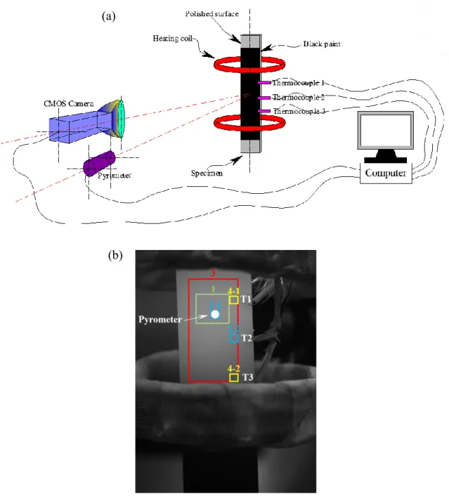
Fig. 1(a) shows the experimental set-up. This set-up consists of several main elements: (a) a steel specimen with the black paint coating; (b) an induction heating device; (c) a 8bits CMOS camera (Viewworks VC-12MC) with 4096 × 3072 pixels, mounted with a lens (Nikon ED, 200 mm); (d) a pyrometer and three thermocouples to provide the classical temperature measurement; (e) a computer with the software to record the experimental data (images, exposure time and temperature) and automatically adjust the exposure time to control the image gray level.

The experiment was conducted in a small dark room. The distance between the front lens of the camera and the specimen surface was approximately 1 meter. The CMOS camera was controlled by a home-made Labview software, which could either just control the image acquisition time or also automatically adjust the exposure time of the camera to maintain the mean image gray level of the selected regions stable during the heating process of the specimen. The computer recorded simultaneously the digital images acquired by the camera (with gray level encoded between 0 and 255 level) and exposure times.

Fig. 1(b) shows an acquired image of the specimen surface. The white dot in the center of the image is the measuring position of the pyrometer. T1, T2 and T3 are the measuring positions of three thermocouples. The green rectangle 1 is a chosen ROI 1 with 500 × 400 pixels, analyzed by our homemade software, where the mean gray level is intended to be maintained stable or even constant by automatically adjusting the exposure time. The two blue squares 2-1 and 2-2 are two 100 × 100 pixels areas, chosen to identify the parameters of the radiometric model in this configuration. These two particular areas are chosen because

5

they correspond to the measurement points of the pyrometer and to the location of the thermocouple T2. The red rectangle 3 with 800 × 1700 pixels is a wide region for the thermal field reconstruction. Two yellow rectangles with 100 × 100 pixels are chosen to validate the accuracy of the calculated temperatures, in which the yellow rectangle 4-1 is a region corresponding to the measured temperature by thermocouple 1 (T1), and the yellow rectangle 4-2 is a region corresponding to the measured temperature by thermocouple 3 (T3).

Fig. 1 (a) Experimental set-up and (b) an acquired image of specimen surface: rectangle 1 is the ROI for exposure time adjustment; rectangles 2-1 and 2-2 are considered for the identification of the radiometric model;

(a)

6

rectangle 3 is the area of thermal field reconstruction; rectangles 4-1 and 4-2 are considered for the validation of the reconstructed thermal field.

3. Radiometric model

3.1 Principle of radiometric model

Radiometric model relates the specimen surface temperature to the output signal (gray level) and exposure time. In this study, a special radiometric model with the intensity I_n(T), which is defined as the gray level I(T) normalized by exposure time  , is introduced, and can be given by [23]: ( ) 2 ( ) exp( ) ( ) n w x C I T I T k T T      ₍₁₎ where T is the temperature, C2 is the second Planck’s constant (1.44 × 10-2 m·K). kw is a parameter of the camera which should be determined by the radiometric calibration process. λx(T) is the extended effective wavelength, which is defined by the following equation [24]:

3 1 2 0 2 3 1 ( ) x a a a a T T T T        (2)

where a0, a1, a2, a3, ···, an are parameters dependent of the whole bench configuration camera’s sensor, lens, surrounding objects, etc.), which should be determined by a priori in situ radiometric calibration. Due to the short temperature ranges from 873 K to 973 K in this study, with the description of extended effective wavelength can be achieved with two parameters a0 and a1 [10]. Thus, the radiometric model equation can be expressed as:

2 0 2 1 2

( )

( )

exp(

)

n w

C

a

C

a

I T

I T

k

T

T















(3)

3.2 Radiometric model calibration

In the radiometric model, three unknown parameters kw, a0 and a1 should be obtained by the calibration process. The mean gray level of two blue ROI (Fig. 1(b)) and reference temperatures provided by pyrometer and thermocouple T2 are used for the radiometric model

7

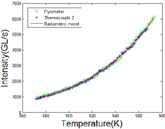
calibration. Experiment data and the calibrated radiometric model of steel specimen surface are shown in Fig. 2. It can be seen that two sets of experimental data obtained by pyrometer and T2 are in good agreement. Based on all these experimental data, the radiometric model (red curve) is calibrated using the least square method, and the three parameters of the radiometric model are obtained and indicated in Table 1.

Fig. 2 Radiometric model of steel specimen surface and experimental data.

Table 1 Three parameters of radiometric model of steel specimen surface.

kw (GL/s) a0 (m-1) a1 (K·m-1)

2.12×1011 _1.20×106 _-3.02×107

4. To maintain image gray level constant

The main disadvantage of near infrared thermography using silicon-based camera is

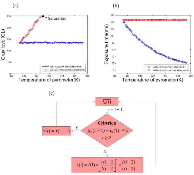
that in near infrared spectral ranges the small variation of temperature causes large modification of image gray level. When the exposure time is maintained constant (red points in Fig. 3(b)), the mean gray level of green ROI 1 (red points in Fig. 3(a)) increases fast from 135 GL to the maximum gray level of 255 GL as the temperature just increases from 873 K to 906 K. As the temperature further increases from 906 K to 973 K, the acquired images are

8

destroyed due to the over saturation of images. These saturated images cannot provide any useful information.

Fig. 3 (a) Mean gray level of ROI 1 evolves with the increase of temperature with/without exposure time adjustment; (b) exposure time evolves with the increase of temperature with/without exposure time adjustment;

(c) flow chart of the approach to maintain the image gray level constant.

The exposure time is related to the duration of acquisition and to the amount of photons collected by the sensor, thus the acquired image gray level can be modified by adjusting the exposure time of the camera. An algorithm based on radiometric model (Eq. (3)), which can adjust the exposure time of camera to maintain the image gray level constant with temperature evolution, is used [25]. The basic equation of radiometric model is an exponential function and the frequency of camera is constant, thus the intensity of a new

(a) (b)

(c) Saturation

9

image ( ( )I i ) can be given by the intensities of the former two image (_n I i _n( 1) and ( 2)I i _n ) based on the specific law of exponential function, which can be given as follows:

2 ( 1) ( ) ( 2) n n n I i I i I i    (4) The Eq. (4) can be expanded as:

2 ( ) ( 1) ( 2) ( ) ( ) ( 1) ( 2) n I i I i i I i i i I i         _{ }      (5)

The objective of this work is to make sure that the mean gray level of new image is equal to that of the first image (I i( )I(1)), thus the new exposure time can be obtained:

2 ( 1) ( 2) ( ) (1) ( 2) ( 1) i I i i I i I i         _{ }      (6)

Flow chart of the approach to maintain the image gray level constant is shown in Fig. 3(c), a criterion equation is introduced to control the adjustment of exposure time:

I i_n(  1) I_n(1) ,i (7) 3 where ( 1)I i _n is the mean intensity of image number i 1, (1)I_n is the mean intensity of the first image, and ε is a critical value chosen by the user. This critical value, as weak as possible, cannot be exactly zero as it is impossible to acquire two exactly identical images in reality (noise, vibrations, optical disturbance, etc.).

Based on this algorithm, a home-made Labview software was produced to automatically adjust the exposure time of the camera to maintain the mean image gray level of selected ROI during the heating/cooling process. If the temperature is maintained constant, the intensity is also constant and the new exposure time (τ(i)) is equal to the former one (τ(i-1)). Otherwise, the new exposure time can be given by Eq. (6).

In this study, the mean gray level of the green ROI 1 is intended to be maintained constant by the homemade software. When the critical value ε is chosen as 0.05 GL/s and the

10

frequency of camera is chosen as 1 Hz, the exposure time after adjustment is indicated by blue points in Fig. 3(b), in which the exposure time decreased with the increasing of temperature. It can be found that the corresponding mean gray level (blue points in Fig. 3(a)) is almost maintained constant as the temperature increases from 873 K to 973 K, indicating that the algorithm and software are feasible and reliable.

5. Reconstruction of thermal fields

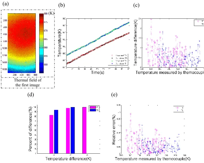
The thermal fields can be reconstructed based on the acquired images and the calibrated radiometric model. As indicated in Section 2.2, the thermal field of the red rectangle region 3 is chosen to be reconstructed. The reconstructed thermal fields of the first image is shown in Fig 4(a), which indicates that the thermal fields of specimen surface are non-homogeneous. Moreover, two thermocouples (T1 and T3) are used to validate the accuracy and reliability of thermal fields, and two yellow rectangles (4-1 and 4-2) are chosen to calculate the temperatures corresponding to these two thermocouples. The temperature of each pixel is calculated by the pixel intensity and the radiometric model, and the mean temperatures of the chosen regions can be also obtained. Fig. 4(b) shows the comparisons between the temperatures measured by thermocouples (T1 and T3) and the calculated temperatures. The calculated temperatures are in good agreement with the measured temperatures. The temperature difference T between the calculated temperature Tcal and the measured

temperature Tmea is also calculated as follows:

 T TcalTmea (8)

Figs. 4(c), (d) and (e) show the temperature differences, the distribution of the temperature differences and relative errors ( 100%

mea

T T

 _

) for T1 and T3, respectively. One can observe that for T1 all temperature differences are less than 2 K, 94% of temperature differences are less than 1 K, and the maximum relative error is about 0.2%. For T3 all temperature

11

differences are less than 2.5 K, 83% of temperature differences are less than 1 K, and the maximum relative error is about 0.3%. These results indicate that the thermal fields reconstructed by this novel method are accurate and reliable.

Fig. 4 (a) Reconstructed thermal field (Unit: K) of the first image; (b) comparisons between measured temperatures and calculated temperatures; (c) the temperature differences between the measured and the

calculated temperatures; (d) distribution of temperature differences; (e) relative error.

6. Conclusions

Some main conclusions can be drawn as follows:

(1) A low-cost high-resolution CMOS camera can be successfully used for temperature measurement after radiometric model calibration.

(a) _{(b) (c)}

Thermal field of the first image

(K)

12

(2) An algorithm based on radiometric model is used to adjust precisely the exposure time of camera to maintain the image gray level constant.

(3) Most of the temperature differences between the calculated temperatures and the measured temperatures are less than 1 K.

(4) Based on this near infrared thermography technique, the accurate and realistic thermal fields on realistic specimen surface in thermal process can be obtained by the image intensity.

References

[1] A.A.Y. AlWaaly, P. Dobson, M.C. Paul, P. Steinmann, Thermocouple heating impact on the temperature measurement of small volume of water in a cooling system, Appl. Therm. Eng. 127 (2017) 650-661.

[2] D.S. Martinez, F. Illan, J.P. Solano, A. Viedma, Embedded thermocouple wal temperature measurment technique for scrapped surface heat exchangers, Appl. Therm. Eng. 114 (2017) 793-801.

[3] S.B. Stankovic, P.A. Kyriacou, The effect of thermistor linearization techniques on the T-history characterization of phase change materials, Appl. Therm. Eng. 44 (2012) 78-84. [4] J.W. Post, A. Bhattacharyya, M. Imran, Experimental results and a user-friendly model of

heat transfer from a thin film resistance temperature detector, Appl. Therm. Eng. 29 (2009) 116-130.

[5] Q. Tang, J. Liu, J. Dai, Z. Yu, Theoretical and experimental study on thermal barrier coating (TBC) uneven thickness detection using pulsed infrared thermography technology, Appl. Therm. Eng. 114 (2017) 770-775.

[6] C. Bu, Q. Tang, Y. Liu, F. Yu, et al., Quantitative detection of thermal barrier coating thinckness based on simulated annealing alogorithm using pulsed infrared thermography technology, Appl. Therm. Eng. 99 (2016) 751-755.

13

[7] S.S. Halkarni, A. Sridharan, S.V. Prabhu, Measurement of local wall heat transfer coefficient in randomly packed beds of uniform sized spheres using infrared thermography (IR) and water as working medium, Appl. Therm. Eng. 126 (2017) 358-378.

[8] D. Soler, P.X. Aristimuno, M. Saez-de-Buruaga, A. Garay, P.J. Arrazola, New calibration method to measure rake face temperature of the tool during dry orthogonal cutting using thermography, Appl. Therm. Eng. 137 (2018) 74-82.

[9] J.H. Tan, E.Y.K. Ng, U. Rajendra Acharya, C. Chee, Infrared thermograpgy on ocular surface temperature: A review, Infrared Phys. Technol. 52 (2009) 97-108.

[10] S. Bagavathiappan, B.B. Lahin, T. Saravanan, J. Philip, T. Jayakumar, Infrared thermography for condition monitoring – A review, Infrared Phys. Technol. 60 (2013) 35-55.

[11] T.L. Liu, C. Pan, Infrared thermography measurement of two-phase boiling flow heat transfer in a microchannel, Appl. Therm. Eng. 94 (2016) 568-578.

[12] P. Tartarini, M.A. Corticelli, L. Tarozzi, Dropwise cooling: Experimental tests by infrared thermography and numerical simulations, Appl. Therm. Eng. 29 (2009) 1391-1397.

[13] T. Sentenac, Y. Le Maoult, G. Rolland and M. Devy, IEEE Trans. Instrum. Meas. 52, 46 (2003).

[14] Y. Rotrou, T. Sentenac, Y. Le Maoult, P. Magnan and J. Farre, Proceedings of ThermoSense XXVII, Orlando, Florida, USA, 2005.

[15] Y. Rotrou, T. Sentenac, Y. Le Maoult, P. Magnan and J. Farre, QIRT J. 3, 93 (2006). [16] S. Dhokkar, B. Serio, P. Lagonotte and P. Meyrueis, Meas. Sci. Technol. 18, 2696

14

[17] K. Mangold, J. A Shaw, M. Vollmer, The physics of near-infrared photography, Eur. J. Phys. 34 (2013) S51.

[18] F. Meriaudeau, Real time multispectral high temperature measurement: Application to control in the industry, Image Vision Comput. 25 (2007) 1124-1133.

[19] D. Teyssieux, D. Briand, J. Charnay, N.F. de Rooij, B. Cretin, Dynamic and static thermal study of micromachined heaters: the advantages of visible and near-infrared thermography compared to classical methods, J. Micromech. Microeng. 18 (2008) 065005.

[20] D. Teyssieux, S. Euphrasie, B. Cretin, Thermal detectivity enhancement of visible and near infrared thermography by using super-resolution algorithm: Possibility to generalize the method to other domains, J. Appl. Phys. 105 (2009) 064911.

[21] D. Teyssieux, L. Thiery, B. Cretin, Near-infrared thermography using a charge-coupled device camera: application to microsystems, Rev. Sci. Instrum. 78 (2007) 034902.

[22] Y. Rotrou, Thermographie courtes longueurs d’onde avec des caméras silicium : contribution à la modélisation radiométrique, Thèse, L’école des mines d’Albi-Carmaux, 2006.

[23] J.J. Orteu, Y. Rotrou, T. Sentenac, L. Robert, An innovative method for 3-D shape, strain and temperature full-field measurement using a single type of camera: principle and preliminary results. Exp. Mech. 48 (2008) 163-179.

[24] P. Saunders, General interpolation equations for the calibration of radiation thermometers, Metrologia 34 (1997) 201-210.

[25] C. Zhang, J. Marty, A. Maynadier, P. Chaudet, J. Réthoré, M.C. Baietto, An innovative technique for real-time adjusting exposure time of silicon-based camera to get stable gray level images with temperature evolution, Mech. Syst. Signal Pr. https://doi.org/10.1016/j.ymssp.2018.12.042.