Ithaque 23 – Automne 2018, p. 75‐96
If God does not explain parsimony,
what does ?
Jonathan St‐Onge
*Although many scholars take parsimony for granted today, Elliott Sober shows in his latest book, Ockham’s Razors, that they might not be rationally justified to do so. In particular, he claims that the famous Ockham’s Razor, the heuristic that says one should not postulate more entities than necessary, rests on some implicit assumptions that go back to Newton and his rules of reasoning. The problem is that Newton justified those basic rules on theological grounds, that is, the world is parsimonious because God is orderly. All is not lost : Sober suggests that two contemporary perspectives from probability theory do justify parsimony. The first one is related to Bayesianism, and the fact that Ockham’s Razor is embedded in Bayes’ theorem. Sober criticizes this view and argues for an alternative, one in which predictive accuracy is more fundamental. I suggest that Sober might be right about the unseen role of predictive accuracy, but that this does not entail that Bayesians should adhere to Sober’s framework. It is my contention that Sober’s case against Bayesian model selection has more to do with the Bayesian worldview than the methodology per se.
The search for parsimony in science and philosophy is often characterized as finding the simplest theories that best carve nature at its joint. One way to justify it is through Ockham’s razor, the heuristic that says one should not postulate more entities than necessary, so long as the theory keeps explaining the data. There are some issues with this heuristic. In his latest book, Ockham’s Razors (2015), the philosopher of science Elliott Sober shows that a major one has to do with the fact that the widespread use of parsimony in science goes ______________
* L’auteur est étudiant à la maîtrise en philosophie (Université du Québec à
back to Newton and his “Rules of reasoning”. The relevant rules in this context are the following ; (i) No more causes of natural things should be admitted than are both true and sufficient to explain their phenomena (nature does nothing in vain) ; (ii) Therefore, the causes assigned to natural effects of the same kind must be, so far as possible, the same1. The issue is that Newton himself did not really
justify those rules, except for his unpublished commentary on the Book of Revelations in which he writes that simplicity in nature comes from the fact that God is orderly. Since then, many great scientists have appealed to Ockham’s razor for various reasons, but, as Sober points out, the question about what exactly rationally justifies the epistemic relevance of parsimony in science is still open.
The aim of this paper is to critically evaluate two contemporary views of parsimony that arise in the context of model comparison and selection. The first one holds that parsimony is epistemically relevant because it reflects predictive accuracy. In that paradigm, parsimonious models provide more accurate predictions when fitted to old data. This view is put forth by Sober in the second chapter of his book. Second, parsimony is related to the plausibility of a model in Bayesian statistical inference. In that story, parsimony is embedded in the optimal trade-off between accuracy and complexity to avoid overfitting, that is, when models explain perfectly the observed data, but fail to properly predict new data. This paradigm relies heavily on the likelihood function, which conveys how probable some observations are for different settings of a model’s parameters. According to Sober, if we substitute one paradigm for the other as the goal of inference, the epistemological landscape undergoes a fundamental change2. This dramatic change, says Sober, is marked by the fact that,
in the first paradigm, likelihood and parsimony can clash. That is to say, a model can be predictively accurate and confer lower probabilities on the data at hand. When this happens, Sober suggests that we should be reductionists about parsimony ; “If parsimony contributes to the achievement of some more fundamental epistemic goal, I am all ______________
1 Cited in Elliott Sober, Ockham’s Razors : A User’s Manual (Cambridge, Ma :
Cambridge University Press, 2013), p. 33.
2 Elliott Sober, “Bayesianism–its Scope and Limits”, in Bayes’ Theorem, ed.
Swinburne, R, (Oxford : Oxford University Press, 2002), pp. 1-17, here p. 12.
for it. If it does not, I am not. 3” In other words, he claims that
predictive accuracy in model comparison is a more fundamental goal than parsimony as classically understood in the likelihood paradigm4.
Given that model comparison and selection cuts across science and philosophy, parsimony enjoys a privileged position. As Sober makes clear in his book, the case of parsimony is key because it is concerned with what all knowledge should be like. It entails a shared belief that simplicity is somehow desirable. In this context, I examine Sober’s claims that we should privilege predictive accuracy over plausibility when performing model comparison, and thus, we should prefer likelihood comparison above Bayesianism, as proposed by the likelihoodist approach advocated by Sober. Bayesianism is a school of thought in probability theory that adheres to the Bayesian interpretation of probability — that is, the meaning of probability is found in the degree of belief in an event of a rational agent. For Bayesians, probability is fundamentally about uncertainty and our inability to extract ourselves from any given point of view. If Sober is right, Bayesianism fails to recognize that parsimony is not only about likelihoods, and thus needs revisions. I suggest that, first, Sober tends to inflate the differences between Likelihoodism and Bayesianism, but that in principle, there are no reasons why Bayesians could not integrate predictive accuracy in their model comparison, and that, second, there are significant compromises that come with the acceptation of Sober’s likelihoodism which might not be advantageous for Bayesians.
One contribution of this paper will be to bring forth a more hands-on approach in the debate. The way I will do it is to present parsimony as an empirical object as understood by the machine learning community, something that Sober does not talk about. I have chosen this particular focus because I take machine learning to be the modern science of inferring and learning plausible models from observed data, which then can be used to make predictions about ______________
3 Sober, “Ockham’s razors”, p. 149.
4 Although Sober criticizes the likelihoodist, it is important to realize that he
has nothing against likelihood. On the contrary, he advocates that likelihood might be more important than parsimony itself. What he is saying is that we should look at the first paradigm because in the second one parsimony and likelihoods go hand in hand, so we cannot learn about them independently.
future data5. In this context, parsimony is not an abstraction but
rather an empirical result of our experiments with statistical modelling. Given the success of Bayesian methods in machine learning, it is worthwhile to include this complementary aspect in the debate of what rationally justify parsimony.
The roadmap of the paper is as follows. In the first section, I will present Sober’s case for predictive accuracy and Likelihoodism in his book. In the second section, I will describe how model comparison is performed from the (Bayesian) machine learning perspective. I conclude by looking at where Sober does hit the mark about the Bayesian (likelihood) framework, even after integrating the hands-on view of machine learning, and why those criticisms do not seem sufficient for Bayesian to give up their methodologies. That said, model comparison is complicated and thus my argument remains partial.
1. Predictive accuracy in Model Comparison and Likelihoodism
Sober proposes the following example to illustrate how parsimony is relevant for predictive accuracy. Let’s suppose that you sample 100 corn plants each of two fields. In the first sample, says Sober, average height is 52 inches. In the second sample, average height is 56 inches. Then, we need to imagine coming back yet another day to do the same exercise. The key question is to know which of the following two predictions is more accurate : (i) we are going to have the same result (x1= 52 inches and x2 = 56 inches) or (ii) we can lump together the two samples and predict that x = 54 inches. Sober suggests that we give names to the two predictions. I call the first situation H1 to
reflect the one “adjustable parameter” (which Sober calls DIFF, for difference in the two populations) and the second, H0, because there
is no free parameter (which Sober calls NULL). This setup is useful because it leads to the following question : “which model, when fitted to ______________
5 see Zoubin Ghahramani, “Probabilistic machine learning and artificial
intelligence”, Nature 521 (2015) : pp. 452-459, here p. 454. Also, Sober lumps together all Bayesians. But as we know, there are as many interpretations of Bayes' theorem as there are Bayesians. I was curious to know if what Sober wrote about Bayesianism in the context of biology can easily be translated into another domain, machine learning.
the old data you have, will more accurately predict the new data that you do not yet have ? 6”
The key point in the above example is that, if we were only interested in the plausibility of a model, we would think that H1 is
true and H0 is false. Recall that the plausibility of a model is defined
by the optimal trade off between accuracy and complexity, given some observations. Thus, we should expect that a model with an adjustable parameter is more likely than one that presupposes that two populations happen to have exactly the same height (x = 54 inches). Models with adjustable parameters make more flexible predictions, which we can adjust once we have more data. However, if we take predictive accuracy into account, we find ourselves in a situation where H1 has a higher likelihood, but H0 could be more
predictively accurate. For example, if we sample over and over again from the same corn field populations, H0 might be a better guide to
predictive accuracy because it “keeps you to the straight and narrow ; [whereas] DIFF (H1) invites you to stray.” 7 By that Sober means the
null hypothesis forces you to have a good rule, whereas H1gives you
the a more flexible space to make up complex models. Given the possible discrepancy between parsimony and likelihood, Sober claims that we should not limit ourselves to the plausibility of a model. I next use that (overly simple) example to introduce the (likelihoodist) model comparison advocated by Sober.
Before we move on to discuss model comparison, we take a brief detour to examine the Likelihoodism that Sobers advocates. Likelihoodism is an approach to statistical inference that poses itself as a middle ground between frequentism and Bayesianism8.
______________
6 Sober, “Ockhams Razors”, p. 128. 7 Ibid.
8 Note that sometimes, likelihoodists are at war with the frequentists (i.e.
ecology, see Burnham and Anderson 2006 ; Aho et al. 2014). Some other times, likelihoodists want to distinguish themselves from Bayesians (i.e. biology, Forster & Sober 2001 ; Sober 2008). We focus exclusively on the second situation. That said, it is worth noting that one of the main differences between the three is related to the Law of likelihood. Both Bayesians and likelihoodists conform (in different ways, related to their uses of likelihood functions) to the the Law of likelihood, whereas frequentists do not.
Likelihoodists assume that the law of likelihood stands by itself, without making appeal to priors as in Bayesianism. This law states the following : that evidence E favors hypothesis H1 over H2 if and only
if Pr(E|H1) > Pr(E|H2). For example, we could say that a cough
favors the hypothesis that someone has the flu over cancer if and only if Pr(cough|flu) > Pr(cough|cancer). For Sober, this probability statement does not require prior beliefs to make sense. This is key because likelihoodists want the data to “speak for themselves”. To be clear, recall that likelihood is not the same as probability, i.e. the cancer hypothesis can be very likely without being highly probable. Another distinctive feature is that likelihoodists do not like to talk about “catchalls”9. That is to say, likelihoodists do not talk about the
probability of having a cough, given the negation of not having the flu. In epistemology, Sober targets Bayesian model averaging, in which the weighted average of the likelihoods of all the alternative theories must be taken into account10. Conversely, Sober claims that
Likelihoodism is more responsible because it limits itself to only assess well-grounded, specific hypotheses. In brief, Likelihoodism is characterized by the belief that we can access the world as it is, and that should be enough to discuss epistemology.
Sober’s argument for Likelihoodism is both theoretical and political. Sober argues that we should choose to be likelihoodists not only for its theoretical virtues, but also because this is more “scientific” than to appeal to degrees of belief (as Bayesians do) when talking about various hypotheses. In Sober’s words, “Likelihoodism is an epistemology for the public world of science ; it aims to isolate something objective on which agents can agree despite the fact that they differ in terms of their prior degrees of confidence in the hypotheses under consideration.”11 This is meant to contrast with Bayesianism, under
which term Sober lumps all the various flavors under the idea that they are an epistemology for the private world. Moreover, Sober argues that Likelihoodism is more modest because, contrary to Bayesians, likelihoodists do not believe that it is possible to always compute posterior probabilities12. Yet again, likelihoodists claim that statistical
______________
9 Sober, “Ockham’s Razors”, p. 84. 10 Ibid., p. 83.
11 Ibid. 12 Ibid.
inference would be better served by focusing on specific hypotheses favored by the evidence. I will come back to these claims later on. For now, we move on to model comparison under the likelihoodist perspective.
Model comparison is about finding a common measure to compare different models and select the one that best explains the data at hand. This is a much more difficult task than it first appears, as models vary in important ways from domain to domain. For Sober, the solution to model comparison is related to maximum likelihood estimation (MLE). MLE is a statistical method used to find the parameter value that maximizes the likelihood function, given some observations. The resulting parameters are known as “maximum likelihood estimators”. In our corn plant example that point estimation would be the parameter that maximizes the H1
likelihood13. Given our sample means of 56 and 52 inches, the
number that makes the observed difference the most probable is simply the difference between the two, 4 inches. Sober calls that estimate L(H1). It is thought to be a fitted model upon which we can
make predictions about new observations. Note that the common wisdom in this kind of problem is to work with the logarithm of the likelihood function, since it is strictly increasing, and thus we can show that to maximize the likelihood is the same as minimizing the neg log likelihood (i.e. “the maximum likelihood criterion”). This method is well known to have some problems related to parsimony.
One of the main issues with MLE in model comparison is that it tends to systematically pick up the most complex model (the one with more adjustable parameters) as the best one. More parameters entail more flexibility to fit the data at hand. Often, this translates into overfitting, i.e. the inability to effectively predict new data. Once again, in our corn plant example, this means that because we allow our sample means to differ in H1, our model might fail to make precise
predictions about other corn fields. This is why Sober introduces the Akaike Information Criterion (AIC). Information criterion in model comparison is a way to score each model in a way that integrates
______________
13 Given that Ho has no free parameters, the expected mean that would have
complexity by penalizing models that have more parameters. The AIC is central to Sober’s argument and is described next.
The AIC comes from Akaike’s theorem, which is the mathematical formulation that makes the role of parsimony in predictive accuracy explicit for Sober14. The theorem states the
following :
An unbiased estimate of the predictive accuracy of model
Data∨L} –k M = log {Pr 15.
This equation states that predictive accuracy is determined by the log likelihood of a fitted model, in our case L(H0) and L(H1), minus
the number of parameters k (i.e. the penalty for the most complex models, here the fact that H1 has one more than H0). In other words,
there is a trade-off between the goodness of fit of the model (higher likelihood being rewarded) and simplicity (low value for k, achieved by having fewer parameters). The AIC then provides us with two scores, or unbiased estimate, to compare our models.
Akaike’s theorem requires three assumptions ; (i) all sampling comes from the same “underlying reality” ; (ii) this data pool is normally distributed when repeatedly sampled (“regularity assumption”) ; (iii) one of the competing models is considered to be true, or at least close to the truth16. Note that the unbiasedness in the
theorem refers to the estimator that is “centered” on the true value of the quantity being estimated, over long run. This is related to the third assumption, in which ‘truth’ is given by the Kullback-Leibler (KL) divergence (also called relative entropy). This “distance” can be cast as a measure of the number of bits wasted by using an
______________
14 To note, AIC has two important extensions, AICC and TIC (Takeuchi
Information Criterion), that are important to avoid practical problems ; for example, AICC is thought to resolve the problem AIC encounters when a dataset is small. Given that I am interested into the main conceptual idea of AIC, I have decided to not talk about these.
15 Ibid., p. 131. 16 Ibid., pp. 133-4.
approximation instead of the true (unknown) distribution17. In this
context, we aim to find the model that minimizes information loss, given the observations. In summary, Akaike’s theorem provides us with a score (a criterion) based on a model’s predictive accuracy. This score is thought to be tied to parsimony because it penalizes complexity when comparing models of various complexities.
On top of the three assumptions embedded in the AIC, there is one last requirement. The MLE for each parameter must be unique (or “identifiable”). To exemplify what identifiability means, Sober asks us to think about a single data point given by your kitchen kettle (say pressure) and that we use AIC to find how well a linear model would predict that point. There is an infinity of ways that a straight line can fit a single point, making it impossible to infer ‘the’ best fitted model18. This is what is meant by “uniqueness” of a model. For
Sober, this uniqueness entails a limit on how complex a model can be to evaluate the data at hand19. Sober notes that because Bayesianism
only consider the average likelihood, and not the “likelihood of the most likely member of the model20”, it does not require identifiability
and thus have the issues to deal with infinitely complex problem. In summary, if we satisfy all the requirements above, Sober favors the predictive accuracy paradigm because it guarantees a clear-cut criterion to compare similar models that differ only in terms of parsimony, here embedded in the expected performance of models.
As mentioned before, a consequence of this focus on predictive accuracy is that a false model can score better on the AIC than a true model. This unintuitive fact is reflected by another one of Sober’s slogans : “instrumentalism for models, realism for fitted models.”21 Being
instrumentalist here is a synonym for being reductionist about parsimony. The realist part is related to Sober’s idea of closeness to truth, by which he means “a proposition is close to some target proposition that is true.”22 For example, we have the proposition that
______________
17 David Mackay, Information Theory, Inference and Learning Algorithms
(Cambridge : Cambridge University Press, 2003), p. 34.
18 Sober, “Ockham’s Razors”, p. 134. 19 Ibid., p. 135.
20 Ibid. 21 Ibid., p. 144. 22 Ibid., p. 146.
my computer is in my bedroom. Although this is false, because my computer is actually in my office, the proposition is thought to be ‘closer to truth’ than saying that my computer is in Canada. Similarly, a model with no adjustable parameters (like H0) might be false, but if
it is close enough to truth (as measured by KL divergence), the model can be considered more predictively accurate than the true (and more flexible) one. Conversely, a model with adjustable parameters that is true (like H1) might be overlooked because when repeatedly fitted to
old data, and then scored on the basis of predictive accuracy, some of the estimates will deviate from the true value. Hence, Sober claims that AIC is a tool for instrumentalists and realists : (i) it provides evidence for which of two models predict better ; (ii) it provides evidence for which of two fitted models (on average) is closer to the truth. Here is a brief summary :
Predictively accurate (expected performance, as given by AIC) Less predictively accurate TRUE model (as measured by KL divergence)
Intuitive scenario — fitted model is closer to truth and is more predictively accurate
Unintuitive scenario
FALSE model
Unintuitive scenario — a false model that is more predictively accurate
Intuitive scenario
In this first section, we have seen that Sober prefers Likelihoodism because it explains why parsimony is true without the need to resort to priors. More precisely, the AIC reveals that penalizing complexity plays a central role to avoid overfitting and increase predictive accuracy. Although I admit that Sober is probably right to distinguish between the two views of parsimony mentioned above, I suggest that it does not entail that Bayesians should prefer Sober’s Likelihoodism. To see why, we now turn to Bayesian model comparison from the machine learning perspective.
2. Bayesian Model Comparison in Machine Learning
Sober systematically juxtaposes his Likelihoodism to Bayesian Information Criterion (BIC) and Bayesian Ockham’s razor. I begin with the former. BIC and AIC are often introduced together since they look similar. Indeed, BIC is an estimate of the average likelihood of a model that says the following :
Pr − (k) log (n) BIC (M) = 2log
Commentators usually note that the BIC was introduced by Schwartz (1978) and poses a heavier penalty for complexity. However, following Wasserman (2000), Sober argues that AIC and BIC reflect the two different paradigms mentioned above. They have different goals and must be compared on the same basis as the rest of the argument. This view is echoed in the literature23. Interestingly, it is
not clear who actually advocates BIC from the Bayesian side. This criterion is only thought to be one approximation among others for posteriors and marginal likelihoods. Moreover, as Sober himself notes, BIC is not even that Bayesian in nature as it does not depend on priors24. For all these reasons, I say no more on BIC and move on
towards the Bayesian Ockham’s razor.
Before getting into Bayesian Ockham’s razor, a little aside on priors is required. Recall that priors in Bayesian analysis convey our prior beliefs about the phenomenon (or what is called the latent variable) of interest, before any observations are made. As mentioned before, they are controversial. Oddly enough, it seems to boil down to an old debate about realism (objectivity) and rationalism
______________
23 For example, were written about how AIC and BIC are really different
worldviews. See Ken Aho, DeWayne Derryberry, and Teri Peterson, “ Model selection for ecologists : the worldviews of AIC and BIC ”, Ecology 95 (2014), pp. 631-636.
24 Although BIC is not very Bayesian, the criterion is equivalent to some
important results in Bayesian statistics. For example, this is equivalent to the Laplace approximation and the minimum description length (MDL) criterion, both of which are widely used when approximating the marginals.
(subjectivity)25. The following quote captures Sober’s long-held view
about priors in science :
If science is about the objective and public evaluation of hypotheses, these subjective feelings do not have scientific standing [...] A report of the author’s subjective posterior probabilities blends these two inputs together. This is why it would be better to expunge the subjective element and let the objective likelihoods speak for themselves26.
Compare this quote with David Mackay’s views on the same subject, a notorious Bayesian who (willingly) admits not only that Bayesians do make assumptions (just like anyone else) when they specify free parameters, but that they should make no apologies for this. In his words, “there is no such thing as inference or prediction without assumptions.”27 Furthermore, he explains that the modern Bayesian
tends not to take a “fundamentalist attitude to assigning the ‘right’ priors” when making model comparison, and that, “many different priors can be tried ; each particular prior [corresponding] to a different hypothesis about the way the world is.”28 I will say no more
on that controversy, but we should keep in mind that this debate underlies the present discussion.
Bayesian Ockham’s razor is widely used in the sciences that depend heavily on computation, from simulations in physics to decoding neural activity in neuroscience29. In its modern formulation,
Bayesian Ockham’s razor is embedded in Bayes’ theorem30. As such,
this is not as much a theoretical construct as a direct consequence of using Bayes’ theorem. In this context, this is just an empirical fact that ______________
25 This is most certainly an oversimplification of both camps. 26 Sober, “Bayesianism–its Scope and Limits”, p. 12.
27 David Mackay, “Information Theory”, p. 34. 28 Ibid.
29 See for example Kevin Knuth et al., “Bayesian evidence and model
selection“, Digital Signal Processing 47, (2015), pp. 50-67 ; Karl Friston and Will Penny, “NeuroImage Post hoc Bayesian model selection“, NeuroImage 56 (2011), pp. 2089-2099.
30 Mackay, “Information Theory” ; Iain Murray and Zoubin Ghahramani, “
A note on the evidence and Bayesian Occam’s razor ”, Gatsby Unit Technical Report (2005) : pp. 1-4.
simpler models (as provided by Bayes’ theorem) tend to make precise predictions when learning models from data. Note that there is a risk of confusion here. Sober says that this kind of prediction, which is based on the plausibility of a model, is different from the prediction problem solved by the AIC31. I hope to make this distinction clear by
presenting Bayesian Ockham’s razor as taught in machine learning. The first step in Bayesian modelling is to plug in the relevant models (H1and H0 in the corn plant example), and the priors over the
parameters of those models (the averages associated with H1 and H0),
in Bayes' theorem. Then, if the problem is simple enough, we compute the posterior beliefs that we should entertain about the model’s parameter, given the observations. This procedure can be written in the following way :
p (w ∨ D , H) = p (D ∨ w , H) p (w ∨ H) / p (D ∨ H)
Where H is the model (the probability distribution over the observed data), D is the data (or observations), and w is the parameters. At the first level of inference (i.e. model fitting, or parameter inference), we simply assume a model to be true and we infer the parameters with the posterior probability. At the second level of inference, the one we are interested in for model comparison, the relevant quantity becomes the marginal likelihood (also called the “model evidence”). As claimed by Sober, at this stage we wish to infer the most plausible model given the data and because the marginal is an integral, we effectively average over models. The posterior probability of each model can be written as follows :
p (H ∨ D) ∝ p (D ∨ H) p (H)
(posterior) (likelihood x prior)
This is simply Bayes' theorem reformulated32. Note that the ratio
of two marginals p(D|Hi)/p(D|Hj) is known as the Bayes factor33.
______________
31 Sober, “Ockham’s Razors”, p. 144.
32 Many authors often note that if we assume no preference by assigning
equal chances to the priors, then model comparison p(m|D) is proportional to the likelihood of a model p(D|m). In practice, though, subjective priors are chosen if needed.
Then, to compare different models we need to compute their respective marginals :
p (D ∨ H) = ∫ p (D ∨ w , H) p (w ∨ H) dw
The right hand side of the equation is the definition of the marginal that we can obtain via the sum and product rules in probability theory. Now, we focus on the many interpretations of what the marginal means. An information theoretic definition is that the log2 of (1/p (D ∨ H)is equivalent to the number of bits of
surprise at observing data D under hypothesis H34. Another one,
closer to our discussion, is that the marginal is the probability of generating the data set D from a model whose parameters are sampled at random from the priors35. In that sense, the automatic Ockham’s
razor is just the fact that an overly simple model (narrow distribution, or small variance) has low probability of generating the data set D, while an overly complex one (broad distribution, or large variance with many parameters) explains very little of the data as a whole (see fig 1). In fig 1, note that the marginal is on vertical axis while the horizontal axis reflects all the possibilities of the given data set. The most parsimonious model (in red/pink) is the one that offers the best blend, i.e. the probability mass that best captures (generate) the observed data. This is how the marginal is thought to reflect a preference for simpler models ; namely, higher model evidence (the
33 Bayes factor (also called odds ratio) is thought to be the main way
Bayesians do model comparison. This is the law of likelihood but for Bayesian purposes. The full form it usually takes is P(H1|E)/P(H2|E) = P(D|H1)/P(D|H2) x P(H1)/P(H2). That said, the automatic Ockham’s razor is embedded in evaluating the evidence P(D|Hi) so I have decided to focus on that.
34 Ghahramani, “Probabilistic machine learning”, p. 453.
35 Christopher Bishop, Pattern Recognition and Machine Learning (New York :
Springer, 2006), p. 162. Also note that this idea of generating the data set from our priors is thought to be very useful in machine learning. Indeed, generative models are useful to learn features in general (Hinton 2006). This sampling approach is absent from the toolbox if we limit ourselves to an approach like Likelihoodism.
marginal) will favor the model that most likely would have had generated the data at hand.
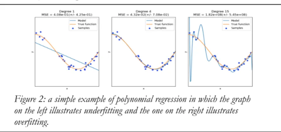
To illustrate how the marginal is embedded in Bayes' theorem, we can think of a simple curve fitting exercise. In the figure below (see fig 2), we have some data points plotted on various graphs whose underlying structure we wish to uncover through inverse (Bayesian) inference. In this simple example, the graph on the left can be thought as an overly simple model. So much so that the ‘model evidence’ may not even resemble the green line in fig 1. The graph on the right is an example of overfitting ; namely, a model with too many parameters for the data. If we were to compute the marginal likelihood of this model, the probability mass would spread all over the data space, similar to the cyan line above. Note that this is different from the problem encountered when optimizing likelihood, as there is no “fitting” of the model to the data36. The blue line is the
model, or hypothesis, that here we know is the true function. Given that all the probability distributions are normalized, we know that this model would be the one with higher “evidence”. As in fig 1, this is
______________
36 Ghahramani, “Probabilistic machine learning”, p. 454.
Figure 1: an illustration of Ockham’s razor from the machine learning perspective. Taken from Ghahramani 2011)
“just right” when the marginal is the highest given the data set D. This is why the marginal can be cast as an automatic Ockham’s razor.
Sober claims that we should prefer Likelihoodism to Bayesianism because posteriors are often intractable, and thus it is better to constrain ourselves to a specific hypothesis37. Sober is right in that the
marginal (and the related posterior) is often not computable—it can be a high dimensional integral and/or contain unknown latent variables that need to be marginalized out38. That said, there are many
techniques to get around this problem that are widely used and empirically successful39. For example, variational inference is an
approximation method that puts a lower bound on the model evidence. In a nutshell, the main idea is to make use of the previously seen KL divergence to minimize the distance (or maximize mutual information)40 between the approximation and the true marginal
distribution. This trick entails that we turn an intractable inference into an optimization problem, which we hope is solvable via different ______________
37 Sober, “Ockham’s Razors”, p. 84. 38 Mackay, “Information Theory”, ch. 33.
39 David Blei et al., “Variational Inference : A Review for Statisticians”, Journal of the American Statistical Association 112, (2017) : pp. 1-41 ; Martin J. Wainwright and Michael I. Jordan, “Graphical Models , Exponential Families , and Variational Inference”, Machine Learning 1 (2008) : pp. 1-305.
40 In Information theory, mutual information measures the dependencies
between two random variables. This is the answer to the question : if I learn A, how much more do I know about B ?
Figure 2: a simple example of polynomial regression in which the graph on the left illustrates underfitting and the one on the right illustrates overfitting.
algorithms41. The lower bound means that if the KL distance
becomes null, then the approximation is the marginal. Interestingly, variational methods require the same toolkit as the AIC to get to a true distribution. Does this similarity means that both methods are related to one another ? This question is a good segue into assessing how Bayesian model comparison relates to Sober’s criticism.
The KL divergence is an information theoretic tool that ‘measures the distance’ between any two probability distributions. Hence, the fact that variational methods in Bayesian model comparison and AIC share the same toolbox does not mean anything per se42. In Bayesian
model comparison, the true distribution being approximated is the marginal—the probability that randomly selected parameters from priors would generate the data at hand. In AIC, the score is based on which fitted model best approximates the true distribution that generates the data. Recall that Sober is realist for fitted models, and instrumentalist for predictive accuracy. Thus, Sober is right to say that Bayesianism, even in machine learning, does not seem to explain why fitted models make different predictions from plausible models. Plausibility in Bayesian model comparison is indissociable from higher likelihoods43.
In the corn plant example, we could pick a model that is good at generating the two distributions, but in doing so, we fail to detect a complementary layer of parsimony hidden away in the comparison of expected performance. Ultimately, Sober seems to be right on this point, “predictive accuracy isn’t the same as fit-to-old-data, nor is it the same as the model’s probability of being true”44. Nothing in the
model evidence of Bayesian model comparison seems to capture the supplementary layer of parsimony as currently provided by the AIC. ______________
41 Bishop, “Pattern Recognition”, ch. 10.
42 That said, Sober often talks of the AIC as a kind of magic bullet because it
is an information criterion. The fact variational methods were developed in Bayesian model comparison can be thought to take the informational gloss off the AIC and Likelihoodism.
43 In Sober’s book, this is why we should think common ancestry is more
parsimonious than the model of multiple ancestors. The former hypothesis is simply more parsimonious because it is more plausible than the second. For Sober, this idea is particularly well developed in the work of Hans Reichenbach on parsimony.
That said, I do not think that this means we should accept the whole likelihoodist story.
Overall, Sober criticised Bayesian model comparison on two main points : priors (especially subjective priors and noninformative priors)45 and the use of average likelihoods instead of looking at
specific hypothesis. We acknowledge that Bayesians should be using something like the AIC to take into account predictive accuracy. Does this mean that we should stop inferring and comparing plausible models via Bayesian model averaging ? At least in the context of this paper, the short answer seems to be the negative. One way to motivate this answer is to look at some of the trade-offs incurred by endorsing Likelihoodism. A common criticism against the AIC is that it does not take into account the uncertainty in the model parameter46. Indeed, the penalty for complexity in the AIC is fixed.
The role of uncertainty is key to motivate the role of averaging in Bayesian accounts, a fact that Sober ignores when he criticizes model averaging. Bayesians maintain that even the most sensible models retain uncertainties at different levels in prediction tasks (i.e. in measurement noise, in parameters and their value, and in the general structure of the model), whereas Sober implies that if we were to limit ourselves to specific hypotheses, the law of likelihood (within the AIC) would guarantee certainty in model comparison47. In other
words, there is a disagreement on the nature of how models represent ______________
45 Noninformative priors are priors thought to be objective, in the sense that
they attempt to capture ignorance and to be like the frequentist approach. They are supposed to “let the data speak by themselves”. As I understand it from the Machine learning perspective, the problem is that you cannot make Bayesian model comparison with them because they do not necessarily add to one. So they are not widely used in model comparison. Instead, many authors are just comfortable with subjective priors. Also note that this is an example where we should not lump together all Bayesians, especially, as it is the case with Sober, when some arguments are specific to those using uninformative priors.
46 Bishop, “Pattern Recognition”, p. 217 ; William D. Penny, “NeuroImage
Comparing Dynamic Causal Models using AIC , BIC and Free Energy.” NeuroImage 59, no. 1 (2012), p. 319–330, here p. 321.
47 This is closely intertwined with the idea that epistemology cannot do, and
should not do, the economy of the cognitive sciences that underlie scientific inquiries.
the world. Bayesians consider models as part of a greater network that is highly dynamic, and as such averaging is favored, while likelihoodists view models like entities, which can be ‘closer to truth’ or not.
There is another way to motivate why Bayesians should stick with model averaging. In a recent paper, Greg Gandenberger proposed that the concept of evidential favoring that is at the heart of the law of likelihood can only be epistemologically relevant within a Bayesian or a frequentist framework48. His argument has two steps. First, any
statistical approach that aspires to become mainstream should provide guidance for beliefs and actions. Although likelihoodists usually dissociate the question of what to believe and do and what the evidence says49, they admit that if there are strong enough scientific
evidence (i.e. objectively well-grounded priors) one can subscribe to those. For likelihoodists, well grounded-priors might be a prior distribution that “comes from a model of the “chance set-up” by which those hypotheses obtained their truth values.”50 A coin tossing
device in which trials can be repeatedly conducted to a obtain sequence of event is an example of chance set-up. It is not obvious that most hypotheses in science satisfy this criterion. Second, Likelihoodism fails to accommodate cases where there is no well-grounded priors without falling into Bayesianism or frequentism51. In
summary, if likelihoodists fail to provide a viable alternative to scientific inquiry, then Bayesians are allowed to be skeptical about Sober’s proposal to adopt his Likelihoodism.
______________
48 Greg Gandenberger, “Why I am Not a Likelihoodist”, Philosophers’ Imprint
16 (2016) : pp. 1-22.
49 Richard R. Royall, “Statistical Evidence : A likelihood paradigm”, (Boca
Raton : Chapman & Hall/CRC, 1997) ; Elliott Sober, “Evidence and Evolution : The Logic Behind the Science”, (Cambridge : Cambridge University Press, 2008), pp. 412.
50 Gandenberger, “Why I am Not a Likelihoodist”.
51 In his paper, Gandenberger goes through a number of various ways that
likelihoodists might resolve the dilemma. They all fail to provide a satisfying middle way to statistical inference as used in science. Ultimately, this is not obvious at all how likelihoodists could achieve that without falling into something like objective Bayesianism.
In conclusion, we have examined two approaches to model comparison and two conceptions of parsimony. I argued that we can dissociate the approaches from the paradigms. Sober is right to point out that the Bayesian model comparison, through the analysis of the model evidence, does not seem to capture parsimony in predictive accuracy — when model comparison is done on the expected performance of a fitted model. As such, there is space for revision and further investigations on the subject matter. That said, this revision does not entail that we should favor Likelihoodism when we assess the plausibility of a model. The argument given by Sober to prefer Likelihoodism reflects a particular view about objectivity in the scientific world more than model comparison per se. For Sober, if we let the data speaks for themselves, we do not need to represent uncertainty. Because Bayesians see model comparison through the lens of uncertainty, they feel the need to be transparent about their assumptions. For them, uncertainty is intrinsic to any kind of inference, and parsimony is a practical tool that is especially useful to avoid overfitting.
Bibliography
Aho, Ken, Derryberry, De Wayne, and Peterson, Teri. “Model selection for ecologists : the worldviews of AIC and BIC.” Ecology, vol. 95, n.° 4(March 2014) : p. 631–636.
Bishop, Christopher. Pattern Recognition and Machine Learning. New York : Springer, 2006.
Blei, David M., Kucukelbir, Alp, and Mcauliffe, Jon D. “Variational Inference : A Review for Statisticians.” Journal of the American Statistical Association, vol. 112, n° 518 (December 2017) : p. 1–41, doi: arXiv:1601.00670v7.
Burnham, Kenneth P., and Anderson, David R. “Sociological Methods & Research.” Sociological Methods Research, vol. 33, n° 2 (2004) : p. 261–304, doi: 10.1177/0049124104268644.
Forster, Marc, and Sober, Elliott. “How to Tell when Simpler More Unified , or Less Ad Hoc Theories will Provide More Accurate Predictions.” The British Journal for the Philosophy of Science, vol. 45, n° 1 (1994) : p. 1–35.
Forster, Marc, and Sober, Elliott. “Why Likelihood ?” In The Nature of Scientific Evidence, edited by M. Taper and S. Lee, p. 153–165. Chicago : University of Chicago Press, 2004.
Friston, Karl, and Penny, William. “NeuroImage Post hoc Bayesian model selection.” NeuroImage, vol. 56, n° 4 (2011) : pp. 2089–2099, doi: 10.1016/j.neuroimage.2011.03.062
Gandenberger, Greg. “Why I am not a likelihoodist.” Philosophers Imprint, vol. 16, no. 7 (may 2016) : p. 1–22.
Ghahramani, Zoubin. “Bayesian nonparametrics and the probabilistic approach to modelling.” Philosophical Transactions of the Royal Society A, vol. 371, (2013) : p. 1–27, doi: 10.1098/rspa.00000000.
Ghahramani, Zoubin. “Probabilistic machine learning and artificial intelligence.” Nature, vol. 521, (May 2015) : p. 452–459.
Wainwright, Martin J., and Jordan, Michael I. “Graphical Models, Exponential Families, and Variational Inference.” Machine Learning, vol. 1, nos. 1-2 (2008) : p. 1–305, doi: 10.1561/2200000001. Knuth, Kevin H., Habeck, Michael, Malakar, Nabin K., Mubeen,
Asim. M., and Placek, Ben. “Bayesian evidence and model selection.” Digital Signal Processing, vol. 47, (2015) : p. 50–67. Mackay, David. J. C. “A Practical Bayesian Framework.” Neural
Computation, vol. 4, n° 1 (1992) : p. 448–472.
Mackay, David. J. C. Information Theory, Inference, and Learning Algorithms. Cambridge : Cambridge University Press, 2003.
Murray, Iain, and Ghahramani, Zoubin. “A note on the evidence and Bayesian Occam’s razor.” Gatsby Unit Technical Report, vol. 2, (August 2005) : p. 1–4.
Penny, William D., Stephan, Klaas E., Mechelli, Andrea, and Friston, Karl J. “Comparing dynamic causal models.” Neuroimage, vol. 22, (2004) : p. 1157–1172.
Penny, William. D. “NeuroImage Comparing Dynamic Causal Models using AIC , BIC and Free Energy.” NeuroImage, vol. 59, no. 1 (2012) : p. 319–330.
Rasmussen, Carl E., and Ghahramani, Zoubin. “Occam’s Razor.” Advances in Neural Information Processing Systems, vol. 13, (2001) : p. 1–7.
Royall, Richard. Statistical Evidence : A Likelihood Paradigm. London : Chapman & Hall, 1997.
Sober, Elliott. “Bayesian - Its Scope and Limits.” In Bayes theorem, edited by S. Swinburne, p. 1–17. Oxford : Oxford University Press, 2002.
Sober, Elliott. Evidence and Evolution : The Logic Behind the Science. Cambridge : Cambridge University Press, 2008.
Sober, Elliott. Ockham’s Razors : A User’s Manual. Cambridge : Cambridge University Press, 2015.
Wasserman, Larry. “Bayesian Model Selection and Model Averaging.” Journal of Mathematical Psychology, vol. 44, (2000) : p. 92–107, doi: 10.1006 ?jmps.1999.1278.