HAL Id: hal-00905055
https://hal.archives-ouvertes.fr/hal-00905055v2
Preprint submitted on 5 May 2014
HAL is a multi-disciplinary open access
archive for the deposit and dissemination of
sci-entific research documents, whether they are
pub-lished or not. The documents may come from
teaching and research institutions in France or
abroad, or from public or private research centers.
L’archive ouverte pluridisciplinaire HAL, est
destinée au dépôt et à la diffusion de documents
scientifiques de niveau recherche, publiés ou non,
émanant des établissements d’enseignement et de
recherche français ou étrangers, des laboratoires
publics ou privés.
Back-pressure traffic signal control with unknown
routing rates
Jean Gregoire, Emilio Frazzoli, Arnaud de la Fortelle, Tichakorn
Wongpiromsarn
To cite this version:
Jean Gregoire, Emilio Frazzoli, Arnaud de la Fortelle, Tichakorn Wongpiromsarn. Back-pressure
traffic signal control with unknown routing rates. 2013. �hal-00905055v2�
Back-pressure traffic signal control
with unknown routing rates
Jean Gregoire∗ Emilio Frazzoli∗∗ Arnaud de La Fortelle∗∗∗ Tichakorn Wongpiromsarn∗∗∗∗
∗Mines ParisTech, Paris, France
∗∗Massachusetts Institute of Technology, Boston, USA
∗∗∗
Mines ParisTech, Paris, France; Inria Paris-Rocquencourt, France arnaud.de la [email protected]
∗∗∗∗
Thailand Center of Excellence for Life Sciences, Thailand [email protected]
Abstract: The control of a network of signalized intersections is considered. Previous works proposed a feedback control belonging to the family of the so-called back-pressure controls that ensures provably maximum stability given pre-specified routing probabilities. However, this optimal back-pressure controller (BP*) requires routing rates and a measure of the number of vehicles queuing at a node for each possible routing decision. It is an idealistic assumption for our application since vehicles (going straight, turning left/right) are all gathered in the same lane apart from the proximity of the intersection and cameras can only give estimations of the aggregated queue length. In this paper, we present a back-pressure traffic signal controller (BP) that does not require routing rates, it requires only aggregated queue lengths estimation (without direction information) and loop detectors at the stop line for each possible direction. A theoretical result on the Lyapunov drift in heavy load conditions under BP control is provided and tends to indicate that BP should have good stability properties. Simulations confirm this and show that BP stabilizes the queuing network in a significant part of the capacity region. Keywords: road traffic, traffic lights, traffic control, transportation control, queuing theory, back-pressure, network control.
1. INTRODUCTION
In today’s metropolitan transportation networks, traffic is regulated by traffic light signals which alternate the right-of-way of users (e.g., cars, public transport, pedes-trians). Congestion is a major problem resulting in a loss of utility for all users due to delayed travel times over the network Shepherd (1992). That is why it is of high interest to find a control policy that can stabilize a net-work of signalized intersections under the largest possible arrival rates. Under traffic light control, a particular set of feasible simultaneous movements, called a phase, is decided for a period of time Papageorgiou et al. (2003). Controlling a traffic light consists of designing rules to decide which phase to apply over time. Pre-timed policies activate phases according to a time-periodic pre-defined schedule, and the signal settings can be fixed by optimiza-tion, assuming within-day static demand Cascetta et al. (2006); Miller (1963); Gartner et al. (1975). They are not efficient under changing arrival rates which require tive control. Many major cities currently employ adap-tive traffic signal control systems including SCOOT Hunt et al. (1982), SCATS Lowrie (1990), PRODYN Henry et al. (1984), RHODES Mirchandani and Head (2001), OPAC Gartner (1983) or TUC Diakaki et al. (2002). These systems update some control variables of a configurable
pre-timed policy on middle term, based on traffic mea-sures. Control variables may include phases, splits, cycle times and offsets Papageorgiou et al. (2003). More re-cently, feedback control algorithms that ensure maximum stability have been proposed both under deterministic arrivals Varaiya (2013), and stochastic arrivals Varaiya (2009); Wongpiromsarn et al. (2012). These algorithms are based on the so-called back-pressure control presented in the seminal paper Tassiulas and Ephremides (1992) for applications in wireless communication networks and require real-time queues estimation. An optimal back-pressure traffic signal controller (BP*) is presented in Wongpiromsarn et al. (2012) and Varaiya (2009). They are defined under different modelling assumptions but they are algorithmically equivalent. The key benefit of back-pressure control is that it can be completely distributed over intersections, i.e., it requires only local information and it is of O(1) complexity. However, the strong assump-tions of the model in Varaiya (2009) (and also implicitly in Wongpiromsarn et al. (2012)) is that controllers require routing rates and a measure of the number of vehicles queuing at every node of the network for each possible routing decision. However, in reality, apart from the prox-imity of the intersection, vehicles (going straight, turning left, turning right, etc.) are all gathered, and it is difficult to estimate the number of vehicles queuing for each
di-rection (see Figure 1). Cameras can give good estimations of the total number of vehicles queuing at a given node, but not the direction of vehicles. However, it is feasible to detect if there are some vehicles (or no vehicle) that want to go to a given destination, if we assume the existence of dedicated lanes from the proximity of the intersection with loop detectors at the stop line.
Dedicated lanes indicated by road markings
Fig. 1. Dedicated lanes for turning vehicles. The dedicated lanes are indicated by road markings when vehicles approach the intersection. Apart from the proximity of the intersection, vehicles are all gathered.
The back-pressure control proposed in this paper(BP) requires such loop detectors and an estimation of the total number of vehicles queuing at each node (gathering all possible directions). It does not assume any knowledge of routing rates. We evaluate the performance of BP with regards to the optimal BP* control. The contribution of the paper is to provide a back-pressure traffic signal con-troller based on more realistic assumptions on the available measurements than state-of-the-art back-pressure traffic signal control and to show in simulations that stability is conserved in a significant part of the capacity region. The paper is organized as follows. Section 2 describes the queuing network model. Sections 3 is mainly expository: it describes BP* highlighting its stability-optimality. The contributions of the paper are presented in Section 4 and 5. Section 4 exhibits BP and a theoretical result on the Lyapunov drift that tends to indicate that it should have good stability properties. The simulations of Section 5 confirm this and show that BP stabilizes the network in a significant part of the capacity region. Section 6 concludes the paper and opens perspectives.
2. MODEL
As standard in queuing network control, time is slotted, and each time slot maps to a certain period of time during which a control is applied. It is convenient to use a fixed pre-defined time slot length, whose size corresponds to the minimal duration of a phase. When the time slot size is fixed, the traffic signal control problem consists of computing at the beginning of each time slot t the phase to apply during slot t. The network of intersections is modelled as a directed graph of nodes (Na)a∈N and links
(Lj)j∈L. Nodes represent lanes with queuing vehicles, and
links enable transfers from node to node: this is a standard queuing network model.
It is a multiple queues one server queuing network. Every signalized intersection is modelled as a server managing a
N2 N1 Q1 Q2 C4 N4 C3 Q3 Q4 N3 C8N8 C7 Q7 Q8 N7 C6N6 C5 Q6 Q5
J
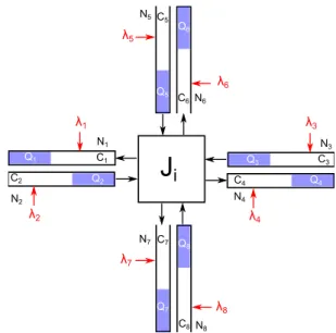
i λ1 λ2 λ5 λ6 λ4 λ3 λ7 λ8 N5 C1 C2Fig. 2. A junction with 4 incoming nodes and 4 outgoing nodes which corresponds to the intersection depicted in Figure 3.
junction which consists of set of links. Junctions (Ji)i∈J
are supposed to form a partition of links. For every junction J, I(J) and O(J) denote respectively the inputs and the outputs of J. Inputs (resp. outputs) of junction J are nodes N such that there exists a link L ∈ J pointing from (resp. to) N . The reader should consider the introduction of junctions in the model as an overlay of the queuing network model. For the sake of simplicity, we do not represent links in the queuing network representation of Figure 2.
Every server maintains an internal queue for every in-put/output, and server work enables to transfer vehicles from an input to an output of the junction. The internal queue at node Na is a vector Qa and Qab(t) denotes
the number of vehicles in the queue of node Na
enter-ing Nb upon leaving Na. The aggregated queue length
Qa(t) =
P
bQab(t) denotes the total number of vehicles
at node Na considering all possible routings after exiting
Na. In this paper, queues are supposed to have infinite
capacities: there is no blocking (see Gregoire et al. (2013a) for an adaptation of back-pressure traffic signal control in the context of finite capacities).
At every time slot t, servers work, resulting in vehicles transfers. Under phase-based control, the transmission rate offered by servers are set by activating a given signal phase pi at each junction Ji from a predefined finite set of
feasible phases Pi at every time slot t. Let P = Qi∈J Pi
denote the set of feasible global phases. Each global phase p = (pi)i∈J ∈ P results in a different service matrix
µ(p) where µab(p) represents the transmission rate offered
by servers to transfer vehicles from Na to Nb in a time
slot when phase p is activated. The transmission rate is assumed to be binary, µab(p) ∈ {0, sab}: it is zero or it
equals the saturation rate sab. Only the vehicles which
are at a node at the beginning of time slot t can be transferred from that node to another node during slot t. Figure 3 depicts the 4 typical phases of a 4 inputs/4 outputs junction.
N1 N2 N3 N4 N5N6 N7 N8 N1 N2 N3 N4 N5N6 N7N8 N1 N2 N3 N4 N5N6 N7N8 N1 N2 N3 N4 N5N6 N7N8 (a) (b) (c) (d)
Fig. 3. A typical set of feasible phases at a junction. For example, supposing that service rates equal 0 or 1, the non zero service rates for phase (a) are µ31, µ36, µ24
and µ27
Exogenous arrivals occur at every node of the network. Let Aa(t) denote the number of vehicles that exogenously
arrive at node Na during slot t. The arrival process Aa(t)
is assumed to be rate convergent with long-term arrival rate λa ≥ 0. When a quantity of vehicles arrives at node
Na ∈ I(Ji) during slot t, exogenously and endogenously, it
is split and added into queues Qab, b ∈ O(Ji). The routing
process is exogenous and assumed to be rate convergent with ratios rab with Pbrab ≤ 1 (see the supplementary
material Gregoire et al. (2013b) for more details). Exits are modelled by assuming that the routing matrix is non-conservative. 1 −Pbrab represents the exit rate of
vehicles entering node Na, it is the ratio of vehicles directly
removed from the network when entering node Na, i.e.
not added to any queue Qab. Note that the only variable
that is controlled is the activated phase at every time slot t, denoted by p(t), and yielding a service matrix µ(p(t)) during slot t.
3. BP* CONTROLLER 3.1 The controller
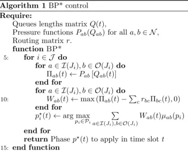
In the following, we expose BP* signal control. It is an ex-tension of the algorithm proposed in Varaiya (2009) where internal/exit links are not differentiated, because exits may occur at any link of the network. It is quite equivalent to the back-pressure controller of Wongpiromsarn et al. (2012), assuming the nodes carry direction information. Loosely speaking, the idea of back-pressure control is to compute pressure at every node based on node occupancy and to open flows which have a high upstream pressure and a low downstream pressure, like opening a tap. Algorithm 1 defines BP* control. At every junction i, for each phase p ∈ Pi, the weighted sum Pa,bWab(t)µab(p)
is computed. Wab(t), the weight associated to transfers
from Na to Nb, is the difference between the upstream
Algorithm 1BP* control Require:
Queues lengths matrix Q(t),
Pressure functions Pab(Qab) for all a, b ∈ N ,
Routing matrix r. functionBP* 5: fori ∈ J do
fora ∈ I(Ji), b ∈ O(Ji) do
Πab(t) ← Pab[Qab(t)]
end for
fora ∈ I(Ji), b ∈ O(Ji) do
10: Wab(t) ← max (Πab(t) −P crbcΠbc(t), 0) end for p⋆ i(t) ← arg max pi∈Pi P a∈I(Ji),b∈O(Ji) Wab(t)µab(pi) end for
returnPhase p⋆(t) to apply in time slot t
15: end function
pressure Πab(t) and the weighted downstream pressure
P
crbcΠbc(t). BP* consists of selecting the phase that
maximizes the weighted sum. Moreover, we assume that in case of equality the selected phase p∗(t) always satisfies µab(p∗(t)) = 0 if Wab(t) = 0.
3.2 Optimal stability
The following theorem states that under linear pressure functions with strictly positive slope, BP* as defined by Algorithm 1 is optimal in terms of stability, i.e. stabilizes the network for all arrivals rates that can be stabilized considering all possible control strategies. It is an exten-sion of the results of Varaiya (2009), because vehicles can enter/exit the network at any node, there is no distinction between exit nodes and internal nodes. Moreover, in con-trast with Varaiya (2009); Wongpiromsarn et al. (2012), pressure functions are just assumed to be linear with strictly positive slope in this paper: Pab(Qab) = θabQab,
θab> 0.
Theorem 1. (Back-pressure optimality). Assuming that pressure functions are linear with strictly positive slopes, BP* as defined by Algorithm 1 is stability-optimal. Proof. Due to space limitations, the full proof is not pro-vided in this paper and is available in the supplementary material Gregoire et al. (2013b). Stability is proved using the Lyapunov function V (t) = V(Q(t)) =Pa,bθabQab(t)2.
The existence of B, η > 0 such that:
E{V (t + 1) − V (t)|Q(t)} ≤ B − ηX
a,b
Qab(t), (1)
enables to conclude stability for the queuing network using the sufficient condition proved in Neely (2003).
4. BP CONTROLLER 4.1 The controller
Back-pressure control proposed in Section 3 requires com-plete knowledge of the queues lengths matrix Q(t) and the routing rates. For our application, a complete knowledge of Q(t) is not realistic because dedicated lanes for turning
vehicles are only from the proximity of the junction. Far-ther, all vehicles are gathered and the controller does not have access to the direction of every vehicle in the absence of vehicle-to-infrastructure communications. That is why we propose in the present paper a controller that uses only the aggregated queues lengths Qa(t) =
P
bQab(t),
i.e. a queue length without direction information. It is defined by Algorithm 2. It computes the phase to ap-ply at every time slot without requiring neither routing rates nor complete knowledge of queues lengths matrix Q(t) and takes as inputs the aggregated queues lengths Qa(t) =PbQab(t). However, it still requires vehicle
de-tectors variables dab(t) ∈ [0, 1] defined below:
dab(t) = min(Qab(t)/sab, 1) (2)
The variable dab(t) can be measured by loop detectors
positioned at dedicated lanes. Algorithm 2BP control Require:
Queues lengths Qa(t),
Pressure functions Pa(Qa),
Loop detectors variables dab(t).
functionBP 5: fori ∈ J do
fora ∈ I(Ji) ∪ O(Ji) do
Πa(t) ← Pa[Qa(t)]
end for
fora ∈ I(Ji), b ∈ O(Ji) do
10: Wab(t) ← dab(t) max (Πa(t) − Πb(t), 0) end for p⋆ i(t) ← arg max pi∈Pi P a∈I(Ji),b∈O(Ji) Wab(t)µab(pi) end for
returnPhase p⋆(t) to apply in time slot t
15: end function
Algorithm 2 defines BP control. Note that for transfers from Nato Nb, the upstream pressure is now Πa(t) and the
downstream pressure is Πb(t): individual queue pressures
Πab(t) are not required. Moreover, the difference between
the upstream pressure and the downstream pressure is multiplied by dab(t) to form Wab(t). Hence, if at time slot
t, there is no vehicle at Na going to Nb, the weight Wab(t)
associated to transfers from Na to Nb vanishes.
4.2 Behaviour of the Lyapunov drift under heavy load conditions
Let us consider the Lyapunov function V(Q) and its evolution through time V (t) defined below:
V (t) = V(Q(t)) =X a θaQa(t)2= X a θa( X b Qab(t))2 (3) Let us define heavy load conditions at time slot t as states of the network such that if the right-of-way is given to any individual queue, it can be emptied at saturation flow, i.e. there are enough vehicles in the individual queue to ensure saturation:
∀a, b ∈ N , Qab(t) ≥ sab (4)
The following theorem proves that under heavy load con-ditions the Lyapunov drift respects the sufficient condition for network stability if λ + ǫ ∈ Λr, for sufficiently large ǫ.
Theorem 2. (Lyapunov drift under heavy load conditions). Assume λ + ǫ ∈ Λr, BP control as defined in Algorithm
2 is applied and the network is in heavy load conditions, then there exists B, η > 0 such that :
E{V (t + 1) − V (t) | Q(t)} ≤ B − ηX
a
Qa(t) (5)
for sufficiently large ǫ.
Proof. Due to space limitations, the full proof is not pro-vided in this paper and is available in the supplementary material Gregoire et al. (2013b).
The above theorem tends to indicate that the network should have good stability properties because the condi-tion for stability is verified in heavy load condicondi-tions for λ sufficiently interior to the capacity region. Unfortunately it does not enable to conclude that the network is stable in a significant part of the capacity region. Indeed, heavy load conditions can not be guaranteed at all time, and when an individual queue Qabis below the saturation flow sab, it is
a constraint for the emptying of Qa, that can unstabilize
the queuing network. Hence, the characterization of the stability region of the queuing network under BP control with the modelling assumptions presented in Section 2 is still a challenging problem. That is why we propose to implement the two back-pressure controllers and to compare their behaviour. The results of the simulations are presented in the next section.
5. SIMULATIONS 5.1 The simulation platform
The model and the algorithms presented in this paper have been implemented into a simulator coded in Java. It simulates a grid network and every junction of the grid has 4 inputs, 4 outputs, and 4 feasible phases as depicted in Figure 3. The height and the width are parameters. Every individual flow allowed by phases of Figure 3 equals 10 (it is the saturation rate). Vehicles are generated at each node Na at an arrival rate λa that can be set as desired.
The arrival process generates individual arrivals as well as batches of 10 vehicles. The routing ratios are fixed at the beginning of the simulation.
5.2 Behaviour of the two back-pressure controllers Simulations have been carried out for a 21×21 square grid network (see Figure 4). First of all, we present simulations results in the case of a network that has been configured with the same arrival rates and routing rates at every node of the network.
Simulation results for a particular network and particular arrival/routing rates The numerical results of Figure 5 correspond to the following parameters. Turn left probabil-ity when a vehicle enters a node: 0.2; turn right probabilprobabil-ity
Fig. 4. The 21 × 21 grid network used for the presented simulations.
when a vehicle enters a node: 0.2; go straight probability when a vehicle enters a node: 0.5; exit probability when a vehicle enters a node: 0.1; probability of a batch: 0.05; pressure functions Pa(Qa) = Qa and Pab(Qab) = Qab
(θa = θab= 1); vehicles are generated at every node with
the same arrival rate λ > 0 that can be set as desired at the beginning of the simulation.
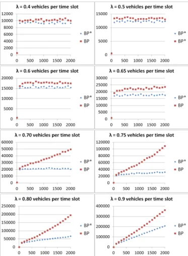
Experiments are carried out at height different arrival rates: λ = 0.4, 0.5, 0.6, 0.65, 0.7, 0.75, 0.8 and 0.9 vehicles per time slot. Figure 5 depicts the global queue of the network over time, i.e. PaQa(t) = Pa,bQab(t), for the
height arrival rates, under BP* control and under BP control. One can observe in Figure 5 that under BP* control, the queuing network is stabilized for λ ≤ 0.7 and gets unstable from λ = 0.75. Under BP control, it is stabilized for λ ≤ 0.65 and gets unstable from λ = 0.7. First of all, it proves that as expected, BP control is not stability-optimal. However, in the particular setting of this experiment, (uniform arrivals/routing rates and grid network), the performance of BP and BP* are very close, and the optimality gap is around 0.05/0.7 ≃ 10%, i.e. a performance of 90%.
However, such a uniform network is not realistic and the results of the next paragraph try to evaluate the performance of BP with regards to BP* with less specific routing/arrival parameters.
Evaluation of BP with regards to BP* on several samples of parameters In the following simulations, the rout-ing/arrival process parameters are not uniform over nodes any more. 10 samples of parameters have been generated. For each sample, the routing/arrival rates are generated as follows. For each direction (straight, left, right), (uni-formly) random values between 0 and 1 are generated, say ys, yl, yr; a (uniformly) random value between 0 and
0.1 is generated for exits, say yω; and the routing rates
are set by normalization of the generated real values, i.e. for the left direction for example, the routing rate is yl/(ys+ yl + yr+ yω). The arrivals rates are set by
generating a (uniformly) random value between 0 and 1 for every node, say λ0
a. At the beginning of the simulation,
a parametrizable scaling value x enables to fix the actual arrival rate of the current simulation: λa = xλ0a, where x
has the same value over nodes. The value of 0.1 for the scale of exits is quite arbitrary and, loosely speaking, fixes
Fig. 5. Evolution of the global queue of the network over time for height arrival rates. Comparison of the behaviour of the network under BP/BP* control. the averaged number of travelled nodes before exiting the network.
Note that the routing rates and the values λ0
a are fixed
for a given sample. However, the value of λa depends on
the value of x set at the beginning of the simulation. The parameter x enables to define a performance for BP with regards to BP* for a given sample. We let x vary and we observe the maximum value of x such that the network is stable under BP versus BP* (say x∗max for BP* and xBPmax
for BP). We define the performance of BP with regards to BP*, or more shortly the performance of BP (because BP* is optimal), as follows:
performance(BP) = xBPmax/x ∗
max (6)
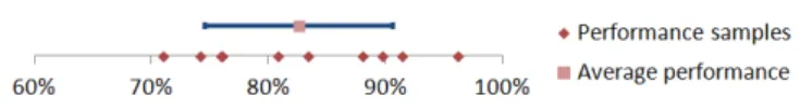
As for previously presented simulations, the probability of a batch is 0.05 and the pressure functions are linear with slope 1. Figure 6 depicts the performance obtained for the 10 samples, the average performance and the standard deviation. The average performance is around 80%, i.e. the optimality gap is about 20%. The simulation results prove that the performance of BP is affected by the rout-ing/arrival rates. Hence, the distribution (over samples) of the performance would be different for a different distribu-tion of routing/arrival rates. Nevertheless, in the particular setting of the experiment, the average optimality gap of 20% seems again a low price to pay with regards to the
much more realistic assumptions on the measurements available to compute the control.
Fig. 6. Performance distribution for ten samples. The point above the axis represents the average performance over samples and the horizontal bar is the standard deviation.
However, these promising results can not be extended to any kind of network of intersections and further simula-tions with a more general structure of network should be carried out to confirm the closeness of performance. We are currently implementing our algorithms in a traffic simulator in order to test the performance of BP control with real traffic data of the city of Singapore.
6. CONCLUSION AND PERSPECTIVES The simulation results of this paper prove that BP is not optimal but tend to indicate that it stabilizes the queuing network in a significant part of the capacity region. The benefits of BP originate from the more realistic assumptions on queues measurements. Computing the phase to apply only requires aggregated queues lengths estimation that can be provided by cameras, and loop detectors at dedicated lanes. The optimality gap, around 20% in the particular setting of the experiments, seems a low price to pay for the benefits of relaxed assumptions on the available measurements. However, simulations have been conducted in a grid network, which is a particular structure, and with synthetic data which can strongly differ from real traffic data. To confirm the closeness of performance, simulations should be carried out in a more advanced traffic network simulator.
Finally, the emergence of vehicle-to-infrastructure commu-nications opens avenues to enhance traffic signal control. The traffic signal controllers can have access, in particular, to the destination node of every vehicle. As a result, back-pressure control with a multiple-commodity queuing net-work model, as proposed in Neely (2003) in the context of wireless communication networks, should be investigated.
ACKNOWLEDGEMENTS
This work was supported in part by the Singapore Na-tional Research Foundation through the Future Urban Mo-bility Interdisciplinary Research Group at the Singapore-MIT Alliance for Research and Technology.
REFERENCES
Cascetta, E., Gallo, M., and Montella, B. (2006). Models and algorithms for the optimization of signal settings on urban networks with stochastic assignment models. Annals of Operations Research, 144(1), 301–328. Diakaki, C., Papageorgiou, M., and Aboudolas, K. (2002).
A multivariable regulator approach to traffic-responsive network-wide signal control. Control Engineering Prac-tice, 10(2), 183–195.
Gartner, N.H. (1983). Opac: A demand-responsive strat-egy for traffic signal control. Transportation Research Record, (906).
Gartner, N.H., Little, J.D., and Gabbay, H. (1975). Opti-mization of traffic signal settings by mixed-integer linear programming part i: The network coordination problem. Transportation Science, 9(4), 321–343.
Gregoire, J., Frazzoli, E., de La Fortelle, A., and Wong-piromsarn, T. (2013a). Capacity-aware back-pressure traffic signal control. arXiv preprint arXiv:1309.6484. Gregoire, J., Frazzoli, E., de La Fortelle, A., and
Wongpiromsarn, T. (2013b). Supplementary mate-rial to: Back-pressure traffic signal control with un-known routing rates. hal preprint hal-00905063. URL http://hal.archives-ouvertes.fr/hal-00905063. Henry, J.J., Farges, J.L., and Tuffal, J. (1984). The prodyn
real time traffic algorithm. In Proceedings of the 4th IFAC/IFORS Conference on Control in Transportation Systems,.
Hunt, P., Robertson, D., Bretherton, R., and Royle, M. (1982). The scoot on-line traffic signal optimisation technique. Traffic Engineering & Control, 23(4). Lowrie, P. (1990). Scats, sydney co-ordinated adaptive
traffic system: A traffic responsive method of controlling urban traffic. Technical report.
Miller, A.J. (1963). Settings for fixed-cycle traffic signals. Operations Research, 373–386.
Mirchandani, P. and Head, L. (2001). A real-time traf-fic signal control system: architecture, algorithms, and analysis. Transportation Research Part C: Emerging Technologies, 9(6), 415–432.
Neely, M.J. (2003). Dynamic power allocation and routing for satellite and wireless networks with time varying channels. Ph.D. thesis, LIDS, Massachusetts Institute of Technology.
Papageorgiou, M., Diakaki, C., Dinopoulou, V., Kotsialos, A., and Wang, Y. (2003). Review of road traffic control strategies. Proceedings of the IEEE, 91(12), 2043–2067. Shepherd, S. (1992). A review of traffic signal control.
Technical report.
Tassiulas, L. and Ephremides, A. (1992). Stability prop-erties of constrained queueing systems and scheduling policies for maximum throughput in multihop radio networks. IEEE Transactions on Automatic Control, 37(12), 1936–1948.
Varaiya, P. (2009). A universal feedback control policy for arbitrary networks of signalized intersections. Technical report.
Varaiya, P. (2013). The max-pressure controller for arbi-trary networks of signalized intersections. In Advances in Dynamic Network Modeling in Complex Transporta-tion Systems, 27–66. Springer.
Wongpiromsarn, T., Uthaicharoenpong, T., Wang, Y., Frazzoli, E., and Wang, D. (2012). Distributed traffic signal control for maximum network throughput. In Proceedings of the 15th international IEEE conference on intelligent transportation systems, 588–595.