Habitat variability and the individual variability of
juvenile Atlantic salmon (Salmo salar)
(La variabilité de l’habitat et du comportement
individuel du saumon Atlantique juvénile (Salmo salar))
par Mathieu Roy
Département de géographie Faculté des arts et sciences
Thèse présentée à la Faculté des études supérieures et postdoctorales en vue de l’obtention du grade de Philosophiæ Doctor (Ph. D.)
en géographie
Juillet 2012
Faculté des études supérieures et postdoctorales
Cette thèse intitulée :
Habitat variability and the individual behaviour of juvenile Atlantic salmon (Salmo salar) (La variabilité de l’habitat et du comportement individuel du saumon Atlantique juvénile)
(Salmo salar)
Présentée par : Mathieu Roy
a été évaluée par un jury composé des personnes suivantes :
Jeffrey Cardille, président-rapporteur André G. Roy, directeur de recherche
James W. Grant, Codirecteur Lael Parrott, membre du jury Jordan Rosenfeld, examinateur externe Jacques Brodeur, représentant du doyen de la FES
Résumé
La variabilité spatiale et temporelle de l’écoulement en rivière contribue à créer une mosaïque d’habitat dynamique qui soutient la diversité écologique. Une des questions fondamentales en écohydraulique est de déterminer quelles sont les échelles spatiales et temporelles de variation de l’habitat les plus importantes pour les organismes à divers stades de vie. L’objectif général de la thèse consiste à examiner les liens entre la variabilité de l’habitat et le comportement du saumon Atlantique juvénile. Plus spécifiquement, trois thèmes sont abordés : la turbulence en tant que variable d’habitat du poisson, les échelles spatiales et temporelles de sélection de l’habitat et la variabilité individuelle du comportement du poisson. À l’aide de données empiriques détaillées et d’analyses statistiques variées, nos objectifs étaient de 1) quantifier les liens causaux entre les variables d’habitat du poisson « usuelles » et les propriétés turbulentes à échelles multiples; 2) tester l’utilisation d’un chenal portatif pour analyser l’effet des propriétés turbulentes sur les probabilités de capture de proie et du comportement alimentaire des saumons juvéniles; 3) analyser les échelles spatiales et temporelles de sélection de l’habitat dans un tronçon l’été et l’automne; 4) examiner la variation individuelle saisonnière et journalière des patrons d’activité, d’utilisation de l’habitat et de leur interaction; 5) investiguer la variation individuelle du comportement spatial en relation aux fluctuations environnementales.
La thèse procure une caractérisation détaillée de la turbulence dans les mouilles et les seuils et montre que la capacité des variables d’habitat du poisson usuelles à expliquer les propriétés turbulentes est relativement basse, surtout dans les petites échelles, mais varie de façon importante entre les unités morphologiques. D’un point de vue pratique, ce niveau de complexité suggère que la turbulence devrait être considérée comme une variable écologique distincte. Dans une deuxième expérience, en utilisant un chenal portatif in situ, nous n’avons pas confirmé de façon concluante, ni écarté l’effet de la turbulence sur la probabilité de capture des proies, mais avons observé une sélection préférentielle de localisations où la turbulence était relativement faible. La sélection d’habitats de faible turbulence a aussi été observée en conditions naturelles dans une étude basée sur des observations pour laquelle 66 poissons ont été marqués à l’aide de transpondeurs passifs et suivis pendant trois mois dans un tronçon de rivière à l’aide d’un réseau d’antennes enfouies dans le lit.
La sélection de l’habitat était dépendante de l’échelle d’observation. Les poissons étaient associés aux profondeurs modérées à micro-échelle, mais aussi à des profondeurs plus élevées à l’échelle des patchs. De plus, l’étendue d’habitats utilisés a augmenté de façon asymptotique avec l’échelle temporelle. L’échelle d’une heure a été considérée comme optimale pour décrire l’habitat utilisé dans une journée et l’échelle de trois jours pour décrire l’habitat utilisé dans un mois.
Le suivi individuel a révélé une forte variabilité inter-individuelle des patrons d’activité, certains individus étant principalement nocturnes alors que d’autres ont fréquemment changé de patrons d’activité. Les changements de patrons d’activité étaient liés aux variables environnementales, mais aussi à l’utilisation de l’habitat des individus, ce qui pourrait signifier que l’utilisation d’habitats suboptimaux engendre la nécessité d’augmenter l’activité diurne, quand l’apport alimentaire et le risque de prédation sont plus élevés. La variabilité inter-individuelle élevée a aussi été observée dans le comportement spatial. La plupart des poissons ont présenté une faible mobilité la plupart des jours, mais ont occasionnellement effectué des mouvements de forte amplitude. En fait, la variabilité inter-individuelle a compté pour seulement 12-17% de la variabilité totale de la mobilité des poissons. Ces résultats questionnent la prémisse que la population soit composée de fractions d’individus sédentaires et mobiles. La variation individuelle journalière suggère que la mobilité est une réponse à des changements des conditions plutôt qu’à un trait de comportement individuel.
Mots-clés : rivière, habitats, saumon, comportement, écoulement, échelles, turbulence, mobilité des poissons, cycles d’activité, utilisation de l’habitat.
Abstract
Spatiotemporal flow variability contributes to create a dynamic habitat mosaic sustaining ecological diversity. One of the most important topics in ecohydraulic research is to identify the relevant scales of flow variability affecting organisms at different life stages. The general objective of the thesis is to examine the links between habitat variability and the behaviour of juvenile Atlantic salmon. More specifically, three themes are addressed: turbulence as a fish habitat variable, the spatial and temporal scales of habitat selection and individual variability in fish behaviour. Through detailed field measurements incorporating a variety of sampling techniques and statistical analyses our objectives were to: 1) Quantify the causal links between standard habitat variables and flow turbulence at multiple scales; 2) Test a new in situ portable flume to analyse the effect of turbulent flow properties on the prey capture probability and foraging behaviour of juvenile Atlantic salmon; 3) Analyse the spatial and temporal scale dependence of fish-habitat associations within a reach during the summer and autumn; 4) Examine individual variation of seasonal and daily activity patterns and habitat use and their interaction; 5) Investigate the individual variation in seasonal daily movement behaviour in relation to environmental fluctuations.
The thesis provides a detailed characterization of turbulence in pools and riffles and showed that the capacity of ‘standard’ fish habitat variables to explain turbulent properties was relatively low, especially at smaller spatial scales, but varied greatly between the units. From a practical point of view, this level of complexity suggested that turbulence should be considered as a ‘distinct’ ecological variable within this range of spatial scales. In a second experiment, using an in situ portable flume and underwater videotaping of fish, we did not conclusively confirm or rule out the effect of turbulence on prey capture probability, but observed a preferential selection of locations where flow velocity was downward and turbulence intensity was lower. The selection of lower turbulence habitat was also observed in natural habitat conditions in an observational field study, in which 66 PIT-tagged fish were tracked for three months in a river reach using a high resolution network of antennas buried in the bed.
Juvenile salmon habitat selection was dependant on the scale of observations. Fish were associated with moderate depth micro-scale habitats, but also with higher depth patch-scale habitats. Furthermore, the range of habitat used by individuals increased asymptotically with the temporal scale. The scale of one hour was considered as optimal to describe the range of habitats used in a day and three days optimal to describe the range of habitat used in a month.
Individual tracking revealed high inter-individual variability in activity patterns, as some individuals were predominantly nocturnal whereas others frequently changed their daily activity pattern. Changes in activity patterns were linked to environmental fluctuations, but also to individual habitat use patterns, which might signify that lower quality habitats require fish to increase daytime activity when food intake and the risk of predation are both high. High inter-individual variability was also observed in the fish movement behaviour. It appeared that most fish exhibited low mobility on most days, but also showed occasional bouts of high mobility. Between-individual variability accounted for only 12-17% of the variability in the mobility data. These results challenge the assumption of a population composed of a sedentary and mobile fraction. Individual variation on a daily basis suggested that movement behaviour is a response to changing environmental conditions rather than an individual behavioural trait.
Keywords : river, habitats, juvenile salmon, behaviour, flow, scales, turbulence, fish mobility, activity patterns, habitat use.
Table of contents
Résumé ... v
Abstract ... vii
Table of contents ... ix
List of tables ... xiv
List of figures ... xvi
Remerciements ... xxviii
Chapitre 1: Introduction ... 1
Chapitre 2: Background ... 7
2.1. Juvenile Atlantic salmon ecology and habitat selection ... 8
2.1.1. Atlantic salmon life cycle... 9
2.1.2. Juvenile salmon foraging behaviour ... 10
2.1.3. Juvenile salmon habitat use and habitat selection ... 12
2.1.4. Behaviour ... 15
2.2. The scales of habitat variability in streams and rivers ... 18
2.2.1. The scales of bed morphology ... 20
2.2.2. The scales of flow variability ... 21
2.2.3. Small-scale river hydraulic variability ... 24
2.3. The effect of habitat on juvenile Atlantic salmon growth and survival ... 31
2.3.1. Metabolic activity costs... 32
2.3.2. Prey availability and distribution ... 36
2.3.3. Efficiency at catching drifting prey... 37
2.3.4. Predation risk ... 41
2.4. Habitat variability and daily activity patterns ... 41
2.5. Habitat variability and habitat selection and mobility ... 50
Chapitre 3: Objectives and methodological approach ... 57
3.1. Problem statement and methodology ... 57
3.1.1. Turbulence as a fish habitat variable ... 58
3.1.2. Spatial and temporal scales of habitat selection ... 60
3.1.3. Individual variability of behaviour... 61
3.3. General methodology ...62
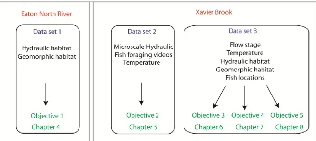
3.3.1. Data set 1: The relationships between ‘standard’ habitat variables and turbulent properties in pools and riffles. ...67
3.3.2. Data set 2: The effect of turbulent flow properties on prey detection and capture probability of juvenile salmon ...68
3.3.3. Data set 3: Individual fish positions and detailed habitat characterization of a reach ...71
3.4. Linking paragraph ...83
Chapitre 4: The relations between ‘standard’ fluvial habitat variables and turbulent flow at multiple scales in morphological units of a gravel-bed river ...85
4.1. Abstract ...85
4.2. Introduction ...86
4.3. Materials and methods ...91
4.3.1. Study site ...91
4.3.2. Field measurements...92
4.3.3. Velocity time series quality check ...93
4.3.4. Habitat variables ...94
4.3.5. Morphological units ...98
4.3.6. Turbulent flow spatial scale partitioning: PCNM analysis ...98
4.4. Results ...104
4.5. Discussion ...109
4.5.1. Spatial scale partitioning of turbulent flow variables ...109
4.5.2. The link between ‘standard’ habitat variables and turbulence at multiple scales ...113
4.6. Linking paragraph ...117
Chapitre 5: The effect of flow properties on the capture probability of juvenile Atlantic salmon in a portable flume ...119
5.1. Introduction ...119
5.2. Materials and methods ...121
5.2.1. Experimental protocol ...125
5.2.2. Flow characterization and flow treatments ...128
5.3. Results ... 131
5.3.1. Effect of flow manipulation on fish foraging ... 132
5.3.2. Flow manipulation ... 134
5.3.3. Preferential focal positions within the flume ... 137
5.4. Discussion ... 142
5.5. Linking paragraph ... 147
Chapitre 6: Spatiotemporal scales of habitat selection of juvenile Atlantic salmon ... 149
6.1. Abstract ... 149
6.2. Introduction ... 149
6.3. Materials and methods ... 154
6.3.1. Study site ... 154
6.3.2. Flatbed antenna grid ... 155
6.3.3. Habitat survey ... 156
6.3.4. Fish capture and tagging ... 158
6.3.5. Data analysis ... 158
6.3.6. Habitat selection analyses ... 159
6.4. Results ... 162
6.4.1. Habitat description ... 162
6.4.2. Fish recordings ... 166
6.4.3. Spatial scales of habitat selection ... 168
6.4.4. Temporal scales of habitat selection ... 172
6.5. Discussion ... 176
6.6. Linking paragraph ... 183
Chapitre 7: Individual variability of wild juvenile Atlantic salmon: effect of flow stage, temperature and habitat use ... 185
7.1. Abstract ... 185
7.2. Introduction ... 185
7.3. Materials and methods ... 188
7.3.1. Study site ... 188
7.3.2. Fish tracking system ... 188
7.3.3. Fish tagging ... 189
7.3.4. Habitat survey ... 190
7.4. Results ...195
7.4.1. Fish recordings ...195
7.4.2. Diel and seasonal activity pattern ...196
7.4.3. Daily activity patterns vs. flow stage and temperature ...199
7.4.4. Diel and seasonal habitat use patterns...200
7.4.5. Diel habitat use vs. activity patterns ...203
7.5. Discussion ...203
7.5.1. Diel and seasonal activity patterns ...203
7.5.2. Individual variability of parr activity ...205
7.5.3. Activity vs. flow and temperature ...206
7.5.4. Seasonal and diel habitat use patterns ...206
7.5.5. Activity patterns and habitat use patterns ...207
7.6. Linking paragraph ...209
Chapitre 8: Individual variability in the movement behaviour of juvenile Atlantic salmon ...211
8.1. Abstract ...211
8.2. Introduction ...211
8.3. Materials and methods ...215
8.3.1. Study site ...215
8.3.2. Fish tracking system...215
8.3.3. Fish capture and tagging ...216
8.3.4. Habitat characterization ...217
8.3.5. Data analysis ...220
8.4. Results ...222
8.4.1. Fish tracking ...222
8.4.2. Behavioural types ...222
8.4.3. Individual variability in behaviour ...226
8.4.4. Temporal variability ...228
8.5. Discussion ...230
Chapitre 9: Discussion and general conclusion ...235
9.1. Summary of key findings ...235
9.3. Turbulence as an important fish habitat variable ... 239
9.4. Scales of habitat selection ... 241
9.5. Individual variability of fish behaviour ... 242
9.6. Concluding remarks ... 243
List of tables
Table 2.1 Habitat use values reported in the literature for Atlantic salmon during the fry stage and parr stage (Armstrong et al. (2003)). ...13 Table 2.2 Field studies examining activity patterns of juvenile salmonids showing
differences between the summer and the winter and between young of the year (YOY) and older juveniles (PYoY). Day, Night and both indicate a predominance of nocturnal, diurnal activity and no particular activity pattern. * Survey carried out during the day only. (I) Individualy tagged ...44 Table 2.3 Laboratory studies examining the effect of various factors on the diel patterns of
juvenile salmonids. Day, Night and both indicate a predominance of nocturnal, diurnal activity and no particular activity pattern. (+) or (-) indicates the direction of the main effect on activity pattern. *Twilight activity unchanged. ...45 Table 4.1 Morphometric characteristics of the units and discharge at the time of flow
velocity sampling. D50 : median size of B-axis (Wolman, 1954). ...92 Table 4.2 All variables of the study in three categories: spatial variables, standard habitat
variables and turbulence variables. Velocity measurements were taken 10 cm above the bed. Spatial average and standard deviations are presented. ...95 Table 4.3 Classification of PCNM variables (PCNMs). Number of variables in each spatial
scales. The physical scale ranges were subjectively set, based on the half periods of the
PCNMs. ...103
Table 4.4 Classification of PCNM variables (PCNMs). Number of variables in each spatial scales. The physical scale ranges were subjectively set, based on the half periods of the
PCNMs. ...106
Table 5.1 Spatially averaged statistics of downstream velocity (U), Reynolds shear stress (τ) and turbulent kinetic energy (TKE) per flow treatment ...129 Table 5.2 Mixed models testing effect of flow treatment on four fish foraging variables. 132 Table 6.1. Class ranges used to compute habitat associations of four variables: Y: water
depth, k: bed roughness, U: downstream flow velocity and TKE: turbulent kinetic energy. Classes were divided evenly over the range of values measured at a stage of approximately 17 cm. ...161
Table 6.2 Mixed model test for day/night period fixed effects. U: mean flow velocity, TKE: turbulent kinetic energy, Y: flow depth, K, bed roughness. ... 173 Table 6.3 Mixed model test for summer/autumn fixed effects for smaller scales (5 min to 24
h) and larger scales (2 to 24 days). ... 174 Table 6.4 Homogeneity of slopes test (GLM ancova). ... 176 Table 8.1 Pearson correlation coefficients of mobility variables versus axis scores from an
ordination of daily fish spatial behaviour in the study reach and proportion of total variance expressed by the two first ordination axes (n=681). ... 224 Table 8.2. Frequency of occurrence (n) and mean (range) of the four mobility variables for
each behavioural type pooled for all individuals. ... 224 Table 8.3 Geometric mean, total sum of squares, and within- and between-individual
variation in four mobility variables and principle component 1 for 24 juvenile Atlantic salmon parr monitored for 6-97 days (619 observations). ... 227
List of figures
Figure 2.1 Schematic representation of how competition and different physical habitat variables affect growth (blue) and predation risk (green) of juvenile Atlantic salmon. Topics of each section of this chapter are identified (red). ...8 Figure 2.2 Atlantic salmon life cycle. See text. (Source: Atlantic salmon federation
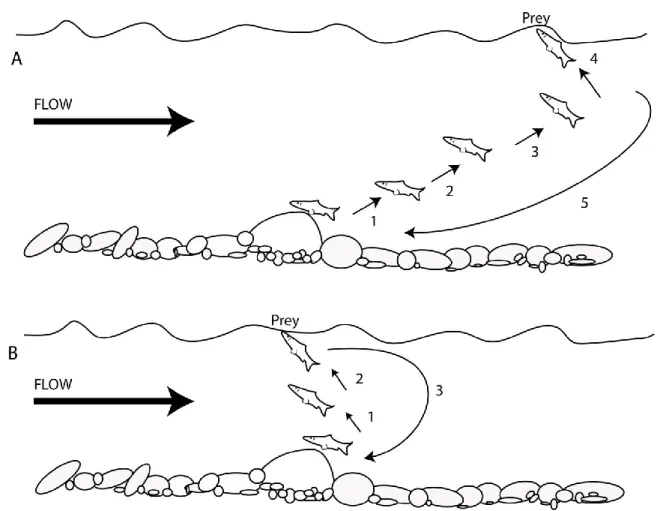
www.asf.ca) ...9 Figure 2.3 Atlantic salmon parr. Art by J.O. Pennanen. Approximately life size. ...10 Figure 2.4 Juvenile salmon surface drift feeding: A) passive indirect. B) Direct. Modified
from Stradmeyer and Thorpe, (1987). ...11 Figure 2.5 Schematic representation of space use of a central place forager. The central
stations are represented by a fish. Solid circles and arrows reprensent foraging or aggressive acts whereas arrows with dashed lines represent shift between stations (Steingrimmson and Grant, 2008). ...17 Figure 2.6 Functional classification of river habitats based on spatiotemporal hierarchy
(Maddock, 1999, after Frissell et al. 1986; Petts, 1984). ...19 Figure 2.7 Hierarchical dynamics of river habitats. Each line represents a landscape scale
divided into patches at different spatial scales. The arrows represent the processes that create interactions between the patches at the same scale and between the scales (Poole, 2002). ...19 Figure 2.8 Schematic representation of a A) temporal and B) spatial velocity power
spectrum in a gravel-bed river. Wo abd W and are channel width and channel depth respectively,H is mean flow depth, Z is distance from the bed and Δ is roughness size (Nikora, 2006). ...23 Figure 2.9 Example of an instantaneous flow velocity time series recorded with an ADV for
a period of 1000 s at a frequency of 25 Hz. u (upper) represents downstream velocity fluctuations, v represents the lateral component and w the vertical component...24 Figure 2.10 Schematic representations of the three types of turbulent flow structures in a
straight section of a gravel-bed river. Vertical exaggeration: 3. Legend: Ejection: burst/ sweep cycle. Echappement : vortex shedding, structure à grande échelle : Large scale flow structure (Buffin-Bélanger et al. 2000) ...25
Figure 2.11 Six flow zones related to the presence of a pebble cluster in a gravel-bed river. Vortex shedding results from the interaction between the recirculation zone and the streamwise flow (Buffin-Bélanger et Roy, 1998). ... 27 Figure 2.12 Snapshot representation of the spatial organisation of the succession of high
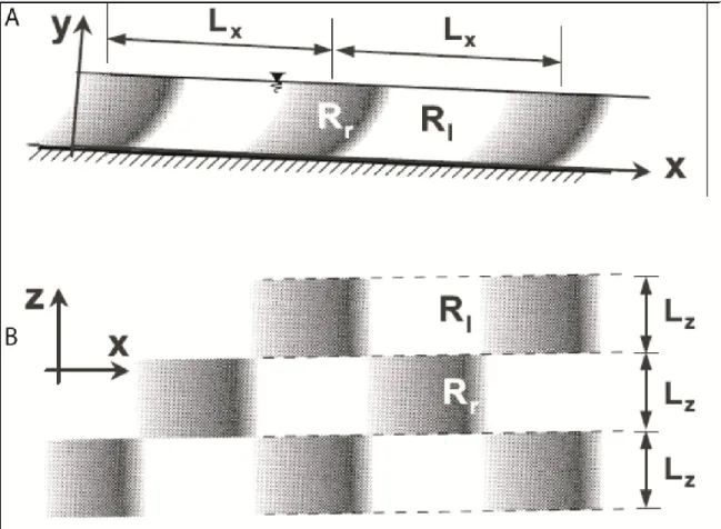
and low-speed wedges. Lx: Length, Lz: Width, Ri:low speed, Rr: high speed. A Side view of the water column. B. Plan view of the river survace (Yalin, 1992). ... 28 Figure 2.13 Conceptual diagram illustrating the levels of internal heterogeneity identified in
glide, riffle and pool biotopes in terms of variation in hydraulic parameters spatially, with relative depth of the measurement and with flow stage (Harvey and Clifford, 2009) ... 30 Figure 2.14 Time series illustrating that axial red muscle activity differs between trout
swimming in free stream flow versus trout holding station behind a cylinder. Circles denote electrode positions with no (open), intermediate (orange), or high (red) muscle activity. (A) A propagating wave of muscle activity for a trout swimming in the free stream. (B) Muscle activity for a trout behind a D-section cylinder with estimated locations of a clockwise vortex (Liao et al., 2003) ... 33 Figure 2.15 Energetic cost values of juvenile Atlantic salmon under four flow conditions
combining (U) and turbulent intensity (RMS). Empty bars represent the energetic costs under low turbulence (5 cm/s) black bars reprensent high turbulence conditions (8 cm/s). Vertical lines represent standard errors (Enders et al. 2003) ... 34 Figure 2.16 The critical swimming speed (open bars) and speed of first spill (hatched bars)
varied across flow treatments. The bars represent the mean while the whiskers represent ±2 s.e.m. Spills (defined as head rotations followed by downstream body translation) were not observed for fish swimming in the control, small cylinder or medium cylinder array flow treatments. SV, MV, LV – small, medium and large vertical; SH, MH, LH – small, medium and large horizontal. (Tritico and Cotel, 2010) ... 35 Figure 2.17 Top view of prey detection location for coho and steelhead at five different
mean flow velocity. Data are pooled (N= 5 fish) for each species. Each circle represent a prey capture. Water flows from the top to the bottom of the figure. Solid lines are mean prey detection angles with 0o upstream of fish and 180o downstream (Piccolo et al. 2008a). ... 38
Figure 2.18 Proportion of time used by the fish for feeding movements in relation to a) mean flow velocity and b) standard deviation of mean flow velocity (i.e. turbulence). Measurements were taken during two sampling period 1 (empty) and 2 (full). The curves (only the data from sampling 2 were considered. (Enders et al. 2005b) ...39 Figure 2.19 The mean (±SE) prey capture probabilities of drift-feeding juvenile brown trout
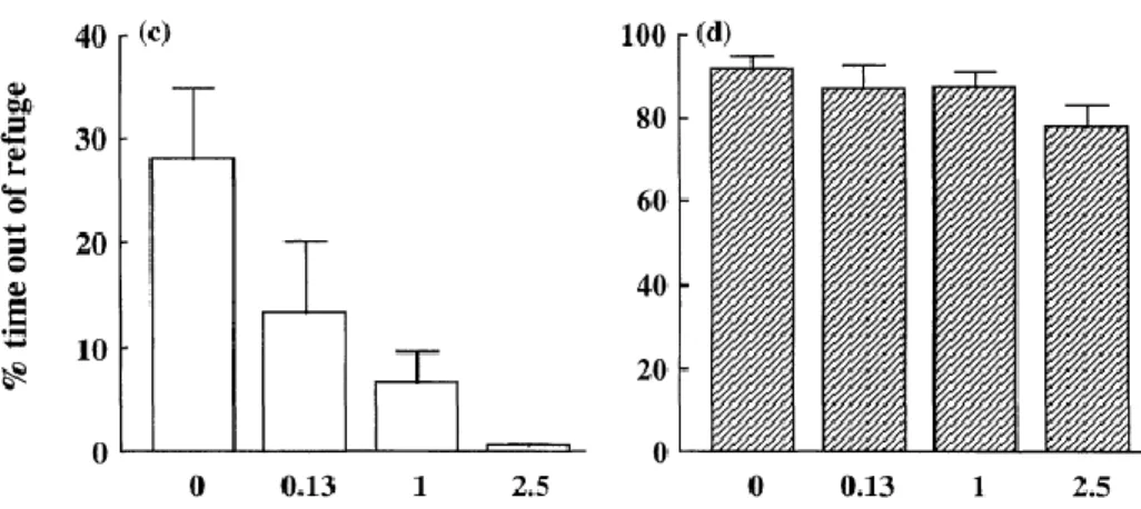
foraging on chironomid larvae at different temperatures (Watz and Piccolo, 2011). ...40 Figure 2.20 Diel activity patterns of juvenile salmon (n=12) in relation to food availability.
Mean (+SE) % of time out of refuge during (left) each day and (right) each night. Food availability expressed as percentage of the wet weight of the fish provided per 24h. (Metcalfe et al. 1999). ...48 Figure 2.21 Fish position in the experimental flume (Black circles) at a discharge of a)
0.030 m3·s-1 and b) 0.111 m3·s-1. Ellipses represents 65% fish presence confidence interval for each discharge treatment. Flow is from left to right (Smith et al. 2005). ..53 Figure 2.22 Relation between Turbulent kinetic energy (TKE) and fish density in a flume
experiment in which juvenile rainbow trout were exposed to different discharges and covers. Closed circles, open circles and inverted closed triangles represent no cover, moderate cover, and full cover, respectively for a discharge of 0.06 m3/s. Closed diamonds, open diamonds and closed triangles represent no cover, moderate cover, and full cover for a discharge of 0.06 m3/s. (Smith et al. 2006) ...54 Figure 3.1 Functional framework within which each of the thesis chapters addresses
specific aspects of juvenile salmon ecology. Physical habitat variables and competition affect the tradeoff between growth and predation risk through components of the energy budget. In turn, behaviour interacts with this tradeoff in order to maximize fitness. Chapter 4: The relations between standard habitat variables and turbulent properties. Chapter 5: The effect of turbulence on the ability at catching prey. Chapter 6: Multiscale habitat selection. Chapter 7 Individual variability in activity patterns and habitat use. Chapter 8: Individual variability in mobility. Interactions between physical habitat variables not shown. ...58 Figure 3.2 Data sets contents (rounded rectangles), obtained at two study sites (rectangles),
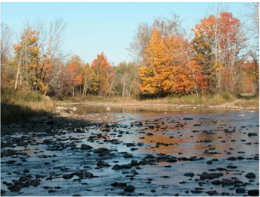
Figure 3.3 Location of the study sites in Southern Québec. Study site 1, Eaton North River is located in the Eastern Townships. Study site 2, Xavier Brook is located at the border between the Saguenay and the Côte Nord region. ... 64 Figure 3.4 Range of scales covered by sampling protocol adopted for each objective. White
bar represent physical habitat sampling and black bars fish sampling. Left side of bars are delimited by grain size (sampling frequency) and right side by extent/duration. “X” indicate the scales of the study (i.e. the window at which the data were averaged). For Objective 3, the temporal scale of minutes represent the duration of sampled velocity measurements. We assumed velocity to remain relatively constant during the study period, as periods of high flow events were removed from the analysis, which explains the lack of correspondence between the fish and the habitat sampling scales for Objective 3. ... 65 Figure 3.5 Study site 1. Eaton North river. Picture taken in August at low flow. ... 67 Figure 3.6 Portable flume installed in the ‘open’ doors position in Xavier Brook, Saguenay
in the summer 2009. Superimposed aluminum graduated frame holds acoustic Doppler velocimeters. ... 69 Figure 3.7 Underwater view of the observation section from camera side. Flow from right
to left. ... 70 Figure 3.8 Study site, Xavier Brook, where a flatbed antenna grid buried in the river bed
was installed. Red spots indicate antenna, suns indicate solar panel and rectangle the location of the controller. Contours illustrate bathymetry at median flow during the summer and autumn 2008. ... 71 Figure 3.9 Schematic diagram of the electronic system. Round and rod antennas (A) are
connected in groups of five to a tuning capacitor unit (T), while rectangular antennas have their own tuning units, which are in turn connected to a multiplexer (M). The multiplexer (M) is linked to the Aquartis controller (AC) containing an Aquartis controller (C), a TIRIS reader (R) and a datalogger (L). The multiplexer and the controller are both connected to a DC converter (Reg) linked to the batteries (B) and solar panels (S). The multiplexer, controller, DC converter and batteries are housed inside a shelter (dotted box). Arrows indicate the flux of information (Johnston et al. 2009) ... 72
Figure 3.10 Reach of Xavier brook where the network of antennas was installed. Study site delimited by red lines. Yellow arrows indicate flow direction. Picture was taken in June at high flow. ...73 Figure 3.11 Network of antennas, as built by Johnston et al. (2009), with locations of the
round antennas (black circles), rectangle antennas (lines) and rod antennas (cross). Arrow indicates flow direction. For the study included in this thesis, the round antennas downstream and in the side channel, the rectangle and the rod antennas were not used. ...74 Figure 3.12 Passive integrated transponder (22mm) ...76 Figure 3.13 Tagging a juvenile Atlantic salmon with a passive integrated transponder.
Closing incision with surgical bound while irrigating gills with water. ...76 Figure 3.14 Definition of components of sampling design. Grain size, interval, extent and
scale. Sampling units are represented as squares and the scale is defined as the area over which values are averaged (Legendre and Legendre, 1998). ...77 Figure 4.1 Color plots of Depth (Y), Mean streamwise flow velocity (U) and turbulent
kinetic energy (TKE) for the four morphohygraulic units Riffle 1 (R1), Riffle 2 (R2), Pool1 (P1) and Pool 2 (P2). Flow velocity was sampled every 25 cm on a regular sampling grid (points). ...100 Figure 4.2 Schematic diagram of Principal component of neighbour matrices (PCNM)
methodology. Step 1: From the spatial coordinates, a matrix of the Euclidian links between the samples was built. Step 2: The distance matrix was truncated at a distance (0.25 m). Step 3: A matrix of eigenvectors was obtained by Principal coordinates analysis of the truncated matrix. Step 4: All positive eigenvectors (PCNMs) were mapped and grouped in spatial scales. The figure presents six examples of PCNMs constructed from the coordinates of Pool 2, selected from each of the spatial scales. XXL: 3-4 m, XL: 2.5-3 m, L: 1.5-2.5 m, M: 1-1.5 m, F: 0.5-1 m, VF: 0.25-0.5 m. The size of the circles is proportional to the magnitude of the PCNMs values. Step 5: Each group of PCNMs associated to a specific scale were used as explanatory variables in canonical analysis (RDA) to explain the variability of turbulent flow variables. Modified from Borcard et al. (2004) ...101 Figure 4.3 The values in rectangles express the total variance explained by all scales
spatial model (XXL: 3-4 m, XL: 2.5-3 m, L: 1.5-2.5 m, M: 1-1.5 m, F: 0.5-1 m, VF: 0.25-0.5 m). ... 105 Figure 4.4 Fractions of explained variance (adjusted R2) for each turbulent flow variable
per spatial scale. PCNMs models: XXL: 3-4 m, XL: 2.5-3 m, L: 1.5-2.5 m, M: 1-1.5 m, F: 0.5-1 m, VF: 0.25-0.5 m. ... 107 Figure 4.5 Fraction of variance (adjusted R2) of ‘scaled turbulence’ explained by habitat
variables (Y: depth (m), U: mean streamwise velocity (cm/s), k: bed roughness index (m)). ‘Scaled turbulence’ represents the first (λ1) and second (λ2) canonical axis of each spatial scale (PCNM models). ... 108 Figure 5.1 a) Plan view of portable flume. Dashed lines represent the positions of wings in
open positions. Camera is held by a support underwater. “O” represents the location of food delivery at mid water column height. X defines the location of a continuously recording ADV. b) Side view of the portable flume with wings closed. For the experiment, width was adjusted to 0.75 m. Removable nets were installed at both ends of the observation section (shaded rectangles). Transversal bars (red) are attached in order to strengthen the flume structure. ... 122 Figure 5.2 Added flow obstacle formed with standard American size bricks (203 x 102 x 57
mm) used to generate turbulence at the entrance of the observation section. ... 123 Figure 5.3 Portable flume installed in Xavier Brook. Camera and velocity probes were
wired to a computer on the bank. Four Acoustic Doppler velocimeters (ADVs) were used to characterize hydraulics within the observation section. ADVs were removed during feeding trials. ... 124 Figure 5.4 Underwater view of the observation section from beside the video camera. Flow
is from right to left. ... 124 Figure 5.5 Four flow treatments carried out in the portable flume: Low velocity Turbulence
1 (wings parallel); Low velocity turbulence 2 (wings parallel with obstacle); High velocity turbulence 3 (wings opened); and, High velocity turbulence 4 (wings opened with obstacle). Flow is from right to left. ... 126 Figure 5.6 Bathymetry contour map (cm) in the observation section. ... 127 Figure 5.7 A) Feeding trials per individual, for which fish were inactive and never started
feeding (fish showed low interest in feeding and performed fewer than 5 feeding excursions) and trials in which individuals were actively feeding. B) Frequency of successful trials (i.e. fish actively feeding) per treatment. ... 131
Figure 5.8 Boxplot of A) prey capture probability, B) aborted prey probability, C) average attack time of prey drifting at 10-25 cm and D) proportion of time resting on the substrate per flow treatment. LVT1: low speed low turbulence, LVT2: low speed high turbulence, HVT3: high speed low turbulence, HVH4: high speed high turbulence. 133 Figure 5.9 Proportion of attacks at low (0-10 cm), medium (10-25 cm) and high (25-40 cm)
height per treatment. ...134 Figure 5.10 Maps of streamwise velocity (cm/s) A) close to the bottom (5 cm above the
bed) B) at mean column velocity (0.4Y) C) and at 0.6Y (25 cm above the bed) for the four flow treatments. ...135 Figure 5.11 Maps of Reynolds shear stress (N·m-2 X10⁻¹) A) close to the bottom (5 cm
above the bed) B) at mean column velocity (0.4Y) C) and at 0.6Y (25 cm above the bed) for the four flow treatments. ...136 Figure 5.12 Maps of bottom downstream flow velocity. (Center) Relative frequency maps
of fish locations (datum =individuals). Flow is from left to right. (Right) Relative frequency of available and used focal mean flow velocity and associated preference index. Positive and negative values illustrate preference and avoidance respectively ...138 Figure 5.13 (Left) Maps of bottom vertical velocity (W). (Center) Maps of longitudinal
Integral time scale (ITSU) at 0.4Y. Flow is from left to right. (Right) Relative frequency of available and used focal vertical velocity (positive values =upward, negative = downward) and associated preference index. Positive and negative values illustrate preference and avoidance respectively. ...139 Figure 5.14 (Left) Maps of bottom Reynolds shear stress. (Center) Relative frequency maps
of fish locations (datum =individuals). Flow is from left to right. (Right) Relative frequency of available and used focal Reynolds shear stress and associated preference index. Positive and negative values illustrate preference and avoidance respectively. ...140 Figure 5.15 (Left) Maps of bottom turbulent kinetic energy (TKE). (Center) (Left) Maps of
TKE at 0.4Y. Flow is from left to right. (Right) Relative frequency of available and used focal TKE and associated preference index. Positive and negative values illustrate preference and avoidance respectively. ...141
Figure 6.1 The study reach, delineated by the white bars , on Xavier Brook, Saguenay, Qc, Canada (location shown by star on inserted map). Bed morphology was characterized by a clear riffle-pool sequence. Maximum bankful width is approximately 35 m. .. 155 Figure 6.2 Time series of water level and water temperature. Gray shading indicates
periods during which river stage was 20 cm over the minimum base level observed during the study period. Vertical dashed line denotes the 12oC diurnal activity suppression threshold defining a warmer summer period and a colder autumn period. Stars indicate the two fish tagging sessions and numbers the flow measurement sessions. ... 163 Figure 6.3 Maps of depth (Y), bed roughness (k) (heterogeneity of bed elevations, see text),
mean downstream velocity (U) sampled at 10 cm above the bed at base flow and turbulent kinetic energy (TKE). Dots represent the sampling locations. ... 165 Figure 6.4 Cumulative curve functions of physical habitat availability F(x) in the study
reach. Y: flow depth, K: bed roughness, U: flow velocity, TKE: turbulent kinetic energy. ... 166 Figure 6.5 Maps of A)Depth (stage:15 cm) B) proportional circles representing the number
of different tagged individuals detected at each antenna over the entire study period C) the frequency of fish detections observed. Frequency of fish detections was estimated from time decimated data (i.e. only one location per hour was kept at a single antenna location, see text). Flow is from left to right. ... 167 Figure 6.6 Fish-habitat associations of juvenile Atlantic salmon over a range of spatial
scales averaged over 98 days for four physical habitat variables Y: depth, k: bed roughness, U: downstream flow velocity and TKE: turbulent kinetic energy. Lines at zero represent null association, closed dots represent a significant negative association whereas open dots represent significant positive associations (M-W test α=0.05). Spatial scales are defined as micro at 0.2 m radius, patch scale at 1.25 m radius and meso scale at 5 m. Unnamed scales show intermediate states. ... 169 Figure 6.7 Average proportion of total depth (Y), bed roughness (k), mean flow velocity (U)
and turbulent kinetic energy (TKE) availability used by fish as a function of temporal scales ranging from a) 5 minutes to 24 days and b) 5 minutes to 6h. ... 172 Figure 6.8 Average proportion of total flow depth (Y), bed roughness (k), mean flow
velocity (U) and turbulent kinetic energy (TKE) availability used by fish as a function of temporal scales ranging from 5 minutes to 24 days represented on a log axis. Dots
represent average range used during the summer and stars average proportions of range used during the autumn. ...174 Figure 6.9 Average proportion of the range of used flow depth (Y), bed roughness (k), mean
flow velocity (U) and turbulent kinetic energy (TKE) availability used by fish as a function of temporal scales ranging from 5 minutes to 24 days represented on a log axis. ...175 Figure 7.1 Flatbed antenna grid buried in the bed of a reach of Xavier Brook. 144 antennas
are displayed in transects (dots), connected to a controller and multiplexer on the bank (rectangle) powered by solar panels (suns). Contours illustrate bathymetry at median flow during the study period. ...188 Figure 7.2 Time series of water level and water temperature. Gray shading indicates periods
during which river stage was 20 cm over the minimum base level observed during the study period. The vertical dashed line denotes 12oC, defining a warmer summer period and a colder autumn period. Asterisks indicate fish tagging sessions and numbers the days of flow measurement. ...191 Figure 7.3 Average probability of fish presence per hour during the summer (stars, N=25)
and autumn (open circles, N=14). Horizontal line shows average periods of daylight during summer and autumn. Quadratic logistic regression models of probability of fish presence as a function of hours during the (a) summer and (b) autumn. Solid lines indicate significant curves, whereas dashed lines non-significant curves. ...197 Figure 7.4 Number of days each fish was present in the reach subdivided into diel activity
pattern adopted by each individual in the (a) summer and (b) autumn. ...199 Figure 7.5 Mean + SE activity (i.e. relative frequency of detection) during (stars) the entire
day (24 h), (diamonds) crepuscular, (circles) night and (square) day periods of Atlantic salmon parr in relation to a) water temperature and flow stage above minimum recorded for a period of three months in the summer and autumn. Each datum was the mean activity for each marked fish at each temperature and flow stage interval. For each increasing temperature category, n = 3, 6, 14, 14, 16, 18, 22, 26, 17 and for flow category n= 17, 27, 25, 25, 20, 12, 12. ...200 Figure 7.6 Average (a) flow velocity and (b) depth used by Atlantic salmon parr in the
summer (stars) and autumn (open circles) per hour. Quadratic regressions of individual average (c) flow velocity and (d) use (c) per hour during the summer (n=25)
(significant relationship: solid, non significant: dashed) and (e) and (f) are the same relationships for the autumn period (n=13). ... 202 Figure 8.1 Water temperature (upper curve) and stage (lower curve) recorded from 24 July
to 30 October 2008. The vertical dashed line divides the study into summer and autumn periods based on a threshold of 12oC. The horizontal dashed line shows the flow stage matching bankfull discharge. *indicates the two fish tagging sessions. .. 218 Figure 8.2 Principal component analysis (PCA) on 50 Atlantic salmon parr daily mobility
variables (N=681) during 97 days. Each dot represents the mobility of an individual on a particular day. Open circles show individual average values for the 24 fish that remained in the reach for six days or more. Polygons delineate behavioural types (stationary, sedentary, floater and wanderer) discriminated by a cluster analysis (K-means) on the daily mobility data: Number of sites, Distance travelled (m), Number of movements and Extent (m). ... 223 Figure 8.3 Typical daily mobility corresponding to four behavioural types. Examples were
selected based on the closest average PCA1 and PCA2 scores for each type: 1-
Stationary: 0 movement (Day 26, Fish 15); 2- Sedentary: 3 movements, 4 sites (Day
61, Fish 50), 3- Floater: 37 movements, 5 sites (Day 32, Fish 37), 4) Wanderer 14 movements, 11 sites (Day 61, Fish 66). Contour shows depth at an estimated discharge of 0.4 m3/s (flow stage: 15 cm). ... 225 Figure 8.4 A) Number of days Atlantic salmon parr stayed in the reach subdivided by
behavioural type. Dashed line indicates the fish that stayed more than 6 days. B) Proportion of days fish showed each of the behavioural types. Most individuals exhibited all types of behaviour during the study period. ... 226 Figure 8.5 Time series of the number of individuals tracked on the study site decomposed
by behavioural types, from 24 July to 30 Oct 2008. ... 228 Figure 8.6 Proportion of fish behaviour exhibited on a daily basis by all individuals in
relation to flow stage: low (0-10 cm, n= 34days), median (10-15, n=34 days), high (15-20 cm, n=13 days), very high (>20 cm, n=16 days). ... 229 Figure 8.7. A) Daily averaged flow depth used per behaviour types pooled for all fish
(unequal number of days per fish). B) Daily averaged depth used, each line representing averages per behaviour types per individual. Five individuals (bold lines) exhibited a relatively higher depth used while adopting floater behaviour. ... 230
If the only tool you have is a Kraken, every problem looks like an excuse to release it.
Remerciements
C’est sur les berges de la rivière Patapédia, il y a belle lurette, que tout a commencé. Alors que j’étais un jeune étudiant en soif d’apprendre, André Roy m’a fait confiance et m’a confié le mandat d’assister une équipe belgoquébécoise de géomorphologues fluviaux et de biologistes. Par la suite, année après année, André m’a toujours fortement soutenu et encouragé. Si aujourd’hui je termine un doctorat, c’est en grande partie grâce à lui. Il a su me transmettre sa passion pour la recherche sur les rivières. Grâce à ses cascades d’idées il et son leadership exceptionnel, il a su entrainer dans son sillon une grande équipe de gens créatifs qui forment presque l’ensemble de la relève au Québec. Un grand merci pour tout André.
At the beginning of the PhD, I met Jim Grant. I was granted the privilege to benefit from Jim’s advices and powerful ecological knowledge. Jim, thanks for your kind and generous help, the meetings saving me from running in circles, the academic support and the detailed revisions.
J’aimerais aussi remercier Normand Bergeron, qui m’a offert l’opportunité de prendre le relais au Ruisseau Xavier, sans quoi cette thèse aurait été toute autre. Je lui suis aussi reconaissant pour m’avoir ouvert les portes de la station de recherche du CIRSA. Merci à Patrica Johnston pour son aide précieuse, pour m’avoir montré à marquer des poissons et pour son amitié. Je remercie aussi Francis Bérubé et Marc-André Pouliot pour leur contribution au développement du Kraken et pour être venus affronter les voraces mouches noires du printemps pour mettre le système en marche. Un merci particulier à Claude Gibeault et Laurence Chaput-Desrochers, qui ont passé plusieurs semaines au fond des bois, gardant leur enthousiasme malgré la lourdeur de certaines expériences et les longues journées. Merci aussi à tous les autres qui m’ont aidé sur le terrain, André Boivin, Nancy Martel, Julie Thérien, René Roy et Marie-Eve Roy, Francis Gagnon, Christine Rozon, Annie Cassista. Je remercie aussi Martin Lambert et Jean-François Myre, pour leur professionnalisme et leur aide précieuse dans le développement et la construction du chenal portatif.
Merci à tous les membres de la Chaire de recherche en dynamique fluviale. Je remercie particulièrement mon amie Geneviève Marquis avec qui j’ai partagé le sentier des longues études graduées. Merci pour l’aide généreuse dans mes débuts avec Matlab, l’aide sur le terrain, avec les instruments, pour les innombrables discussions et pour le soutien dans les moments plus difficiles du doctorat. Merci aussi à Geneviève Ali pour sa présence fort agréable et pour représenter un idéal de talent et de persévérance. Je remercie aussi Jamie Luce pour sa générosité, ses conseils et ses encouragements. Merci aux nombreux autres pour leur soutien à un moment ou un autre dans mon parcours, Hélène Lamarre, Claudine Boyer, Patrick Verhaar, Michèle Tremblay, Mathilde Peloquin-Guay, Laurence Chaput-Desrochers et Éric Hallot. Je souligne aussi l’apport de mon comité doctoral, Lael Parrot et Jeffrey Cardille, particulièrement au début de mon cheminement.
Je désire souligner l’appui des organismes pour le financement de mon projet de recherche, le Conseil de recherche national en science et génie (CRSNG), le Fonds québécois de la recherche sur la nature et les technologies (FQRNT), Géoïde, le Fonds canadien pour l’innovation (FCI), la Chaire de recherche du Canada en dynamique fluviale, la Faculté des études supérieures, la Fondation Bombardier et GEC3.
Enfin, merci à mes proches, mes amis et ma famille qui m’ont encouragé tout au long du parcours. Merci à Magali pour le soutien et la complicité pendant mon examen de synthèse, alors qu’elle prenait les bouchées doubles pour terminer sa thèse. Merci à mes parents pour m’avoir transmis leur curiosité et leur amour de la nature ainsi que pour leur intérêt pour mon cheminement. Enfin, je ne remercierai jamais assez ma douce moitié, Marie-Eve, pour sa patience et son indéfectible soutien et pour les compromis qu’ont nécessité l’accomplissement de ce doctorat.
Chapitre 1: Introduction
Habitat selection is a key process governing the distribution patterns of animals. The study of habitat selection by organisms dates back to the beginning of the century (Grinnel, 1917; Lack, 1933). Since then, the question of how and why animals select a particular habitat has been of great interest to ecologists, as it provides important information on the preferences of a species for a range of environmental variables and their habitat requirements (Rosenfeld, 2003). Such information can be used as a framework to predict animal density and abundance relative to habitat availability (Bovee, 1986).
For juvenile salmonids in rivers, the patchy distribution of individuals and density-dependent growth suggest that the availability of suitable habitat is a limiting factor (Grant and Kramer, 1990). To complete its life cycle, a fish needs to survive and grow, which often depends on its ability to locate the most suitable habitats (Finstad et al. 2011). Fast growth depends on a positive energy budget, whereas high survival depends on minimizing the risk of predation. As the safest habitats do not always provide the highest growth potential, growth and avoiding predators are often viewed as a tradeoff (Metcalfe et al. 1999).
River flow is highly variable in space and time. This heterogeneity contributes to the creation of a dynamic mosaic that sustains ecological diversity in rivers (Statzner, 1981). Physical habitat is mainly characterized by the interactions between flow and bed morphology over a range of scales. Spatial scales range from micro particles to large channel morphology features (e.g. riffles and pools) and temporal scales range from flow turbulent fluctuations to seasonal floods (Biggs et al., 2005; Nikora, 2007). Many rivers are
relatively hostile environments for most life, as high energetic costs are required to withstand the strong turbulent flows (Church, 2007). Stream-dwellers benefit from morphological adaptations (e.g. streamlined shapes, low-resistance surfaces) and plasticity in behaviour (e.g. mobility, activity patterns), to deal with strong flows and varying environmental conditions. Such flexibility in behaviour may also allow individuals to improve their chance of survival by balancing the tradeoff between susceptibility to predators and metabolic demands (Fraser et al. 1995).
Despite the great interest in how animals select habitats in the face of spatiotemporal habitat variability, much work remains to be done to understand how behaviour is matched to environmental fluctuations. As an example, recent field studies provide contrasting results on how fish react to fluctuations in velocity (i.e. turbulence), discharge and temperature. With the emergence of methods allowing to track individual fish at a high temporal frequency, a common result among studies is the high variability in behaviour among individuals (Okland et al. 2004; Ovidio et al. 2007; Breau et al. 2007; Heggenes et al. 2007). Because foraging decisions depend on tradeoffs experienced at the individual level, behaviour will likely vary among individuals rather than being strictly determined by large scale environmental variables such as flow stage or temperature (Bradford and Higgins, 2001). However, few studies have explicitly addressed the temporal within-individual variation in behaviour as opposed to describing general trends for groups of individuals.
The general objective of this thesis is to examine individual fish behaviour in relation to habitat variability, with a particular emphasis on the small-scale flow variability
(i.e. turbulence), as there is accumulating evidence that turbulent flow properties influence fish habitat selection (Smith et al. 2005; Smith et al. 2006; Cotel et al. 2007).
Wild Atlantic salmon parr (Salmo salar L.) was selected as a study species, because of its growing status as a model species for examining fundamental relationships between animals and their environment (Findstad et al. 2011). Furthermore, despite its long-standing cultural and economic importance, Atlantic salmon populations are declining over large portions of its range due to the loss and degradation of fluvial habitats (Parrish, et al., 1998). This alarming situation has generated a need for a better understanding of how wild Atlantic salmon interact with habitat during their freshwater life stage. Ultimately, this knowledge will help to provide management tools to assess potential impacts of stream restoration projects. Through innovative fish tracking and habitat sampling techniques, this thesis is an attempt to advance current knowledge of how habitat and, more specifically, flow spatial and temporal variability at the scale of turbulence and flow stage influence the individual behaviour of Atlantic salmon parr.
The thesis comprises eight chapters. An overview of the existing literature on juvenile salmonids behaviour in relation to habitat over a range of spatial and temporal scales is presented in Chapter 2. This literature review presents and discusses the scales of habitat variability in rivers and several aspects of fish behaviour: habitat selection, foraging, diel activity patterns and mobility. This chapter provides a broad context to understand the relevance of the objectives and results of this thesis. In Chapter 3, the objectives are stated and the general methodology is presented, as the main challenges related to data acquisition and analyses are discussed. The main results of this thesis are found in chapters 4 to 8.
Chapter 4, 6, 7 and 8 are written in journal article format for submission to internationally recognized research journals while Chapter 5 is written in the form of a classic thesis chapter.
In Chapter 4, we quantify the relationships between ‘standard’ fish microhabitat variables and turbulent flow properties in morphological units (i.e. pools and riffles) at multiple scales using a novel statistical technique. We show that the spatial coherence of turbulent flow properties is higher in pools than in riffles. However, the capability of standard habitat variables to predict turbulent properties was low, and variable among units of the same morphological type. Therefore, from a practical point of view, turbulence should be considered as a distinct fish microhabitat variable. This article is now published in River Research and Applications.
In Chapter 5, we examine the effect of velocity and turbulent flow pattern on the foraging behaviour of Atlantic salmon parr using an in situ portable flume. This study combines experimental and field-based approaches in order to develop a new methodology for the study of the foraging behaviour of fish. The relation between turbulent flow properties and behavioural measures were examined: time spent near the river bed; capture and attack time; and, capture probability, as well as preferential focal positions across turbulent flow treatments.
The results presented in Chapter 6, 7 and 8 are based on the use of a large array of antennas buried in the bed of a river reach to monitor the position of Atlantic salmon parr tagged with passive integrated transponders (PIT) over a period of three months from the
summer to autumn seasons. To our knowledge, this system provided one of the most extensive spatial and temporal resolutions of fish tracking ever accomplished, allowing us to examine the individual variability of habitat selection, diel activity patterns and movements in a natural river.
In Chapter 6, we examine the spatial and temporal scales of habitat selection of parr. The results reveal the importance of an intermediate spatial (patch scale) and temporal scale (1 hour, 3 days). We show that scale-dependent habitat selection is more important for mean flow velocity and depth than for bed roughness and turbulence.
In Chapter 7, individual patterns of diel activity and habitat use were examined. Results show a predominantly nocturnal and crepuscular activity pattern. However, a fraction of the fish showed a high temporal variability in activity patterns: some days being diurnal; some days being nocturnal; and, other days being active both day and night. This article has been submitted to Canadian Journal of Fisheries and Applications.
In Chapter 8, we quantified individual patterns of parr daily mobility. We found that within-individual variability in daily movement accounted between 84 and 87% of the mobility variability. These results challenge the assumption of a population composed of a sedentary and of a mobile fraction. Individual variation on a daily basis suggested that fish movements respond to changing environmental and biotic conditions rather than being an individual behavioural trait. This article has been submitted to Canadian Journal of
Finally, Chapter 9 discusses the key findings, outlines the general contribution of the thesis, and proposes research pathways for future studies.
Chapitre 2: Background
Rivers are heterogeneous and complex environments. The interactions between flow and the river bed result in a wide range of flow depths and velocity. Stream-dwellers benefit from such heterogeneity, as it provides for various life functions such as feeding, resting and sheltering. For juvenile salmonids, behaviour is flexible, allowing individuals to select particular habitats and to adapt to temporal changes in environmental conditions (Slobodkin and Rapoport, 1974). Herein, we broadly define behaviour as every action made by organisms in response to their environment, thus including the preferential selection of a particular habitat over another one (Wooton, 1990).
Fish behaviour is governed by a range of factors that are interdependent (Armstrong et al., 2003) and interacting over a range of spatial scales (Roy et al., 2010). This chapter reviews the literature focusing on how physical habitat influences the tradeoff between growth (g) and predation risk (µ) and how it affects in turn juvenile salmon behaviour in terms of habitat selection, activity and mobility patterns (
Figure 2.1). Despite the importance of intra- and inter-specific competition on salmonid ecology and habitat selection (Nislow et al., 2011), a full treatment of this biotic issues is beyond the scope of this thesis and this review. Nevertheless, the role of some biotic habitat factors is discussed, as physical habitat effects on fish are often mediated through biotic habitat.
The review is composed of six sections (
Figure 2.1). The first section provides a brief overview of juvenile Atlantic salmon ecology, including foraging behaviour and habitat selection. The second section describes the range
of spatial and temporal scales of physical habitat in rivers. The third section reviews the various effects of habitat on the components of fish energy budget and on predation risk over a range of scales.
Figure 2.1 Schematic representation of how competition and different physical habitat variables affect growth (blue) and predation risk (green) of juvenile Atlantic salmon. Topics of each section of this chapter are identified (red).
The fourth and fifth sections will address the question of the effect of flow variability and activity patterns on habitat selection and on mobility respectively.
2.1.1. Atlantic salmon life cycle
Atlantic salmon (Salmo salar L.) is an anadromous species. Individuals spend a part of their life in the ocean and come to rivers and streams to reproduce (Figure 2.2). In the late fall, during the spawning season, female lay their eggs in redds, in the substrate where they stay for the winter. In early spring, the eggs hatch and the alevins feed on a nutrient rich yolk sac during the first weeks of their life. After about four weeks, the fish emerge from the substrate and move to shallow, low-velocity habitats, called nursery areas (Armstrong et al., 2003).
Figure 2.2 Atlantic salmon life cycle. See text. (Source: Atlantic salmon federation www.asf.ca)
By the end of the year, they will grow to become parr. At this stage, they are easily recognizable by their vertical dark spots and their pattern of red dots that is unique to each
individual (Figure 2.3). The juveniles grow in the river for a period of two to three years. This period can occasionally extend to up to five years. At the end of this period, parr undergo morphological changes called smoltification in preparation for a life in saline water. After one to three years in the ocean, mature salmon will return to spawn in their natal river. As opposed to Pacific salmon, a significant portion of individuals survive after
Figure 2.3 Atlantic salmon parr. Art by J.O. Pennanen. Approximately life size.
spawning and can reproduce more than once (Bernatchez and Giroux, 1991). In this thesis, we are interested in the parr life stage, as it corresponds to a freshwater life stage during which the fish actively forages.
2.1.2. Juvenile salmon foraging behaviour
During the first years of their life, juvenile Atlantic salmon spend most of their time foraging in order to maximize their growth. When they are not foraging, they shelter in the interstices of the substrate to avoid predation (Armstrong et al., 2003; Finstad et al., 2011). Juvenile salmonids are visual foragers (Hughes and Dill, 1990). The majority of their diet comes from drifting macroinvertebrate (Metcalfe et al., 1997), but they can also feed on benthic organisms, especially at low light levels or when drifting prey are not abundant (Nislow et al., 1998; Amundsen et al., 2000). Parr frequently exhibit a fidelity to a specific rearing micro-habitat, often referred to as a ‘home rock’, ‘home stone’, ‘feeding station’ or
‘foraging station’. Their feeding behaviour involves performing ‘attacks’ on prey as they drift on the water surface or in the water column, or simply by a head-jerk movement when the drifting prey is close by. After each foraging movement, parr tend to come back to their home rock to “sit and wait” for the next prey (Stradmeyer and Thorpe, 1987; Figure 2.4). Like most of the sit-and-wait predators, they must visually detect their prey and have a finite detection range (Piccolo et al., 2008a). While they sit on their home rock, parr deploy their pectoral fins to maintain a position that minimizes their swimming energy expenditures (Kalleberg, 1958).
Figure 2.4 Juvenile salmon surface drift feeding: A) passive indirect. B) Direct. Modified from Stradmeyer and Thorpe, (1987).
The fins act as hydrofoils generating a negative lift. Typically, parr contact the substrate with the tips of their extended pectoral fins while upstream at an angle of 10 to 15 degrees (Arnold, 1991). This oblique posture decreases parr reaction time when initiating feeding movements. At higher velocities, to prevent dislodgement, the angle decreases and the dorsal fin retracts to reduce drag. The presence of negative velocity (countercurrent) on the lee of the home rock also helps to reduce the cost of maintaining position (Facey and Grossman, 1992). However, despite this morphological adaptation, maintaining posture may imply significant energy costs (Webb, 2002).
2.1.3. Juvenile salmon habitat use and habitat selection
Numerous studies have detailed the habitat use and habitat selection of Atlantic salmon parr in relation to physical habitat variables (e.g. Rimmer et al., 1984; Degraaf and Bain, 1986; Heggenes et al., 1990). Early studies described parr rearing mesohabitat as a riffle area with a gravel or cobble substrate (Symons and Heland, 1975). It has been reported, however, that parr are also observed in less typical habitats including pools (Saunders and Gee, 1964), ponds and lakes (Erkinaro and Gibson, 1997) and slow moving, often weedy areas.
Most often, juvenile salmonid habitat selection is characterized at the microhabitat scale through snorkelling observations or electrofishing. The method consists in measuring habitat features at the precise location of a fish caught by electrofishing or observed by snorkelling and comparing them to random values of ‘available’ habitat. Physical habitat is routinely characterized using three variables: streamwise flow velocity (U), flow depth (Y) and substrate size (D). Flow velocity is generally either sampled at a depth of 0.6Y or close
to the bed at the focal point (snout velocity). Parr habitat preference varies considerably among studies (Table 2.1). For example, Symons and Heland (1978) observed a preference of parr for a narrow range of velocities (50-65 cm s-1) whereas Heggenes et al (1990) estimated a much wider range of preference (10-65 cm s-1). Such differences highlight the importance of indirect biotic factors interacting with habitat selection, such as fish density and food availability (Finstad et al., 2011).
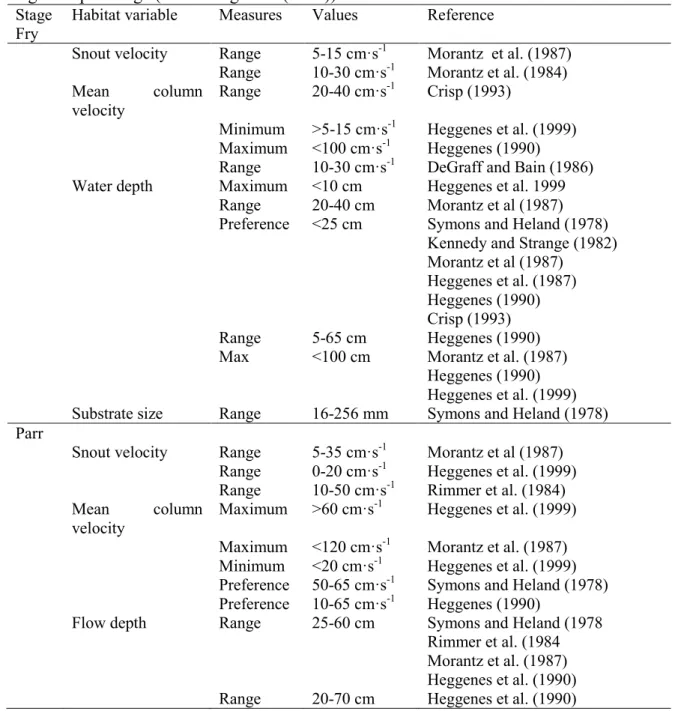
Table 2.1 Habitat use values reported in the literature for Atlantic salmon during the fry stage and parr stage (Armstrong et al. (2003)).
Stage Habitat variable Measures Values Reference Fry
Snout velocity Range 5-15 cm·s-1 Morantz et al. (1987)
Range 10-30 cm·s-1 Morantz et al. (1984)
Mean column velocity
Range 20-40 cm·s-1 Crisp (1993)
Minimum >5-15 cm·s-1 Heggenes et al. (1999) Maximum <100 cm·s-1 Heggenes (1990)
Range 10-30 cm·s-1 DeGraff and Bain (1986) Water depth Maximum <10 cm Heggenes et al. 1999
Range 20-40 cm Morantz et al (1987) Preference <25 cm Symons and Heland (1978)
Kennedy and Strange (1982) Morantz et al (1987)
Heggenes et al. (1987) Heggenes (1990) Crisp (1993) Range 5-65 cm Heggenes (1990) Max <100 cm Morantz et al. (1987)
Heggenes (1990) Heggenes et al. (1999) Substrate size Range 16-256 mm Symons and Heland (1978) Parr
Snout velocity Range 5-35 cm·s-1 Morantz et al (1987)
Range 0-20 cm·s-1 Heggenes et al. (1999)
Range 10-50 cm·s-1 Rimmer et al. (1984)
Mean column velocity
Maximum >60 cm·s-1 Heggenes et al. (1999)
Maximum <120 cm·s-1 Morantz et al. (1987)
Minimum <20 cm·s-1 Heggenes et al. (1999)
Preference 50-65 cm·s-1 Symons and Heland (1978)
Preference 10-65 cm·s-1 Heggenes (1990)
Flow depth Range 25-60 cm Symons and Heland (1978 Rimmer et al. (1984 Morantz et al. (1987) Heggenes et al. (1990) Range 20-70 cm Heggenes et al. (1990)
Substrate Range 64-512+ mm Symons and Heland (1978) Heggenes (1990)
Heggenes et al. (1999)
As these factors vary from site to site, the transferability of habitat preference curves among sites is difficult (Maki-Petays et al., 2002).
Flow velocity is an important factor of habitat selection, as it generates a tradeoff between drifting prey availability and energy costs related to swimming (Fausch and White, 1981; Fausch, 1984; Heggenes et al., 1999). Therefore, in order to maximize energy intake and minimize energy expenditures, parr should select micro habitats where velocity is moderate, yet close to fast currents. Generally, moderate-velocity hydraulic refuges are provided by bed roughness elements, such as protruding boulders. In general, young-of-the-year fish tend to use lower velocity habitats than parr (1+ and older) (Table 2.1), presumably because of their lower capability of catching prey in fast currents (Nislow et al., 1999).
Substrate composition, another important habitat feature, is closely linked to bed roughness, as larger particles are more likely to protrude than smaller particles. Besides affecting the availability of low velocity areas, bed composition also influences the availability of shelter from predation. Hence, parr tend to prefer habitats where the bed is mainly composed of clasts in the cobble to boulder class (64-512 mm) (Heggenes et al., 1999). As parr become larger, they tend to use larger sized rocks as rearing habitats (Mitchell et al., 1998). This preference could also be partly due to an increase in spatial flow heterogeneity providing a greater density of varied habitat types (resting, feeding, sheltering). Recently, it was also shown that the addition of large cobble and boulders could