HAL Id: hal-00130277
https://hal.archives-ouvertes.fr/hal-00130277
Preprint submitted on 10 Feb 2007HAL is a multi-disciplinary open access
archive for the deposit and dissemination of sci-entific research documents, whether they are pub-lished or not. The documents may come from teaching and research institutions in France or abroad, or from public or private research centers.
L’archive ouverte pluridisciplinaire HAL, est destinée au dépôt et à la diffusion de documents scientifiques de niveau recherche, publiés ou non, émanant des établissements d’enseignement et de recherche français ou étrangers, des laboratoires publics ou privés.
Supervised Reconstruction of Biological Networks with
Local Models
Kevin Bleakley, Gérard Biau, Jean-Philippe Vert
To cite this version:
Kevin Bleakley, Gérard Biau, Jean-Philippe Vert. Supervised Reconstruction of Biological Networks with Local Models. 2007. �hal-00130277�
Supervised Reconstruction of Biological
Networks with Local Models
Kevin Bleakleya,1 , G´erard Biaua and Jean-Philippe Vertb
aInstitut de Math´ematiques et de Mod´elisation de Montpellier
UMR CNRS 5149, Equipe de Probabilit´es et Statistique Universit´e Montpellier II, CC 051
Place Eug`ene Bataillon, 34095 Montpellier Cedex 5, France
bCentre for Computational Biology
Ecole des Mines de Paris 35 rue Saint-Honor´e
77305 Fontainebleau Cedex, France
biau,[email protected] [email protected]
Abstract
Inference and reconstruction of biological networks from heterogeneous data is currently an active research subject with several important applications in systems biology. The problem has been attacked from many different points of view with varying degrees of success. In particular predicting new edges with a reasonable false discovery rate is highly demanded for practical applications, but remains extremely challenging due to the sparsity of the networks of interest. While most previous approaches based on the partial knowledge of the network to be inferred build global models to predict new edges over the network, we introduce here a novel method which predicts whether there is an edge from a newly added vertex to each of the vertices of a known network using local models. This involves learning individually a certain subnetwork associated with each vertex of the known network, then using the discovered classification rule associated with only that vertex to predict the edge to the new vertex. Excellent experimental results are shown in the case of metabolic and protein-protein interaction network reconstruction from a variety of genomic data.
1
Introduction
A network, or graph G is an object consisting of a set of vertices (nodes/points) V and a set of edges (lines/links) E that join various vertices in V to other vertices in V . In this paper we only considered undirected graphs with no self-loops, although generalizations to directed graphs are possible. This kind of object is omnipresent in the world around us, such as for example the internet, road networks, electrical networks and social interaction networks. Similarly, various biological systems and processes in the cell can be modelled as graphs upon choosing suitable vertices and edges. The elucidation, analysis and simulation of biological networks has become a major research focus in systems biology.
For example, to discover functional behaviour in the cell, it is of critical interest to know the protein network describing which proteins are functionally related to or interact with other proteins. This can be represented as a network with proteins as vertices, and edges that pass between functionally related or interacting proteins. These networks are, as well as intricate, largely unknown, and even many known networks are to some extent incomplete, with missing proteins and unknown interactions. Experimental discovery of these networks remains a difficult, time consuming and expensive task even with today’s technology, so new complementary methods are being used to try to determine these networks in silico. Given a partially known network, we may try to predict which interactions are missing, which interactions already noted are possibly incorrect, or even whether a new unknown protein should be in the network in a certain place.
One particular example of a protein network is the metabolic network, which can be represented as a graph with enzymes as vertices. Enzymes catalyze chemical reactions, and an edge between two enzymes means that two enzymes catalyze two successive reactions. Figure 1 shows part of one such network, the aminosugars metabolic network, which can be extracted from the KEGG database [10]. Each box represents an enzyme (in the KEGG database it can be clicked on to find information on the enzyme) and each circle represents a chemical compound (which can also be clicked on to provide information about the chemical compound). If two enzymes are separated by one chemical compound, we say they are functionally related.
Recently, there has been considerable interest in the in silico reconstruction of protein networks using a variety of available genomic data. The reason this can be attempted is because there now exist large sets of pertinent biological information about the known enzymes, such as gene expression data, phylogenetic data and location data of enzymes in the cell. The challenge is to use this (copious and often noisy) information in an intelligent way to predict potentially new relationships. Various methods have been suggested to attack network inference problems, such as for protein interaction networks [8], gene regulatory networks [5] and metabolic networks [9]. These methods often use Bayesian [5] or Petri networks [3] or the prediction of edges between “similar” vertices [15, 17]. In fact, most of these methods base their predictions on prior knowledge about which edges should be present for a given set of vertices. This prior knowledge might be based on a model of conditional dependence in the case of Bayesian networks, or the assumption that edges should connect similar vertices.
In the present paper however, as initially suggested by [26], we express the reconstruction task as a supervised learning problem. Often we know the vertices and part of the network, and we would like to use this information to predict the rest of the network. More precisely, given a known (incomplete) graph and information about its vertices, we want to predict the unknown part of the graph. This framework has attracted some attention recently due to its generality and lack of hypotheses regarding the network to be completed or the data available. For example, kernel canonical correlation analysis [26, 27] and kernel metric learning [24] have been proposed to map the genes or proteins onto Euclidean spaces where connected vertices are close to each others; [21] and [11] have expressed the problem as that of filling missing entries in a matrix using an auxiliary matrix, and proposed an algorithm based on information geometry; [1] have formulated it as a classical binary supervised classification problem and solved it with a support vector machine (SVM) based on a specific kernel for edges; [2] tested k-nearest neighbor and SVM classifiers, and provided theoretical justification for the approach. In spite of the important effort devoted to the design of new algorithms, the accuracy of predictions remains questionable. In particular, as the networks of interest are usually sparse, the number of non-interacting pairs far exceeds the number of interacting pairs, and for practical applications one needs predicted edges with a small false discovery rate. As we will see in the experiments, this is far from being the case.
Figure 1: Part of the aminosugars metabolic network, which can be extracted from the KEGG database [10].
All the aforementioned approaches share in common the idea to build a unique model that can be applied to predict whether an edge exists between a new vertex and all existing vertices available during training. Although convenient, this choice might have unwanted consequences: for example, in the approaches of [26, 27] and [24], two nodes close to each other on the known network will tend to have the same predicted neighbors among new vertices; in the approach of [1], two nodes with similar genomic data will have similar predicted neighbors, although they might be in very different places in the training network. Although in some cases such properties might be wanted, the underlying hypothesis (e.g., the fact that genes close to each other on the graph or with similar genomic data are likely to have similar neighbors) are usually not justified nor supported by experimental evidences.
In order to relax these constraints we investigate in the present paper the possibility to build local models to predict the presence or absence of edges with new vertices. More precisely we propose to learn individually a certain subnetwork associated with each vertex of the known network, then use the discovered classification rule associated with only that vertex to predict the edge to the new vertex. Although the price to pay to estimate many local models is that less data is available to train each model, we show on benchmark experiments involving the reconstruction of the metabolic and protein-protein interaction networks that this approach gives in many cases better results than other state-of-the-art methods, validating the approach. Moreover, being a simple collection of pattern recognition problems (one associated to each vertex in the known network) the method is conceptually simple, can in theory be used when one is only interested in the neighborhood of one or a few genes (e.g., for particular pathway elucidation), easily generalizes to the prediction of directed edges, and importantly can straightforwardly take full advantage of the existence of powerful pattern recognition algorithms, such as support vector machines (SVM), which provide a convenient framework to learn from several heterogeneous data sets. In particular we show that a simple scheme for data integration with SVM applied to the integration of various genomic data for the prediction of edges in the metabolic and protein-protein interaction networks provides huge improvements in the performance of the prediction, compared to the use of individual
Figure 2: The supervised learning problem we consider consists in guessing the edges (in dotted line) between vertices in the training set (represented by the 6 circles in the left-hand side of this figure) and vertices in the test set (represented by the 3 circles in the right-hand side of the figure). Edges between vertices in the training sets are known in advance.
genomic datasets. In our benchmark experiment, we estimate that the first predicted edges in the metabolic network from the integration of gene expression profiles, protein cellular localization and phylogenetic profiles, are correct at a false discovery rate level below 10% (i.e., that 90% of the predicted edges are correct), and that we can retrieve about 45% of all correct edges at a FDR level below 50%. While all other methods tested hardly fall below a FDR of 70% for their first prediction, this paves the way for practical use of the predictions, e.g., to experimentally validate the predicted edges.
The paper is structured as follows. In Section 2 we introduce a new method of supervised classification for graphs. In Section 3 we introduce two benchmark data sets and in Section 4 we test the new method and several other state-of-the-art methods on these two data sets. The results are discussed further in Section 5.
2
Methods
2.1
The problem of supervised graph prediction
We consider the problem of predicting new edges in a partially known gene or protein network using side information about the vertices. More precisely we consider the following framework. We assume that a set V of genes or proteins is given, each of them being characterized by genomic data, e.g., expression levels across different experiments or phylogenetic profiles. For the sake of clarity let us assume for the moment that the data can be represented by a real-valued vector, i.e., the gene i is represented by the vector Xi ∈ Rd. We further assume that the restriction of the
graph to a subset V1 of the vertices is known, i.e., that all pairwise edges between two vertices in V1
are observed. The problem consists in predicting the edges between vertices in V1 and vertices in
V2 = V \V1. We call V1 the training set of vertices, and V2 the test set. This framework is illustrated
in Figure 2. Many problems in systems biology can be formulated within this framework, e.g., finding new genes regulated by a transcription factor or finding missing enzymes in a metabolic pathway. We do not consider here the problem of inferring edges between two vertices in the test set, although this could also be of interest for certain applications, because some of the methods we test (in particular the one we propose) do not allow this.
+1
−1
?
?
?
+1
−1
−1
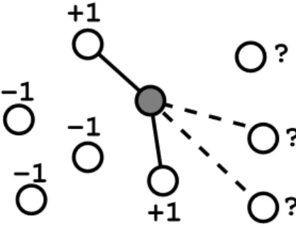
Figure 3: The subgraph of the graph pictured in Figure 2 related to a particular vertex v of the training set (shaded in the picture) induces a {−1, +1}−labelling of the other vertices in the training set, ‘+1’ indicates a vertex directly connected to v and ‘−1’ a vertex not directly connected to v. A classification rule can then be chosen based on this labelling. An edge is predicted from a vertex u in the test set to v if the classification rule predicts a label of +1 for the point u. Ideally, in this picture, we would expect the classification rule to predict a label −1 to the topmost vertex of the test set, and +1 to the two other test vertices, in order to correctly predict the actual edges between v and the nodes in the test set (in dotted line). For clarity, edges between other vertices are not shown.
2.2
Graph inference with local models
We propose to solve the graph inference problem by training several local models to predict new edges linking new vertices with vertices at different positions in the known network. More precisely, we consider first each vertex in the training set v ∈ V1independently. Obviously, every other vertex
in the training set u ∈ V1 is either connected or not connected to the vertex v by an edge. The
crucial idea is thus to take every other vertex u ∈ V1 and give it a label Yu ∈ {−1, +1}, +1 if there
is an edge from v to u, −1 if there is not. We then let a machine learning algorithm for pattern recognition learn a function fv that can assign a label −1 or +1 to any new vertex, in particular
those in the test set V2. Edges are then predicted between v and the vertices in V2 that are given
the label +1. This process is illustrated in Figure 3, and repeated for every vertex v ∈ V1to obtain
a prediction for all candidate edges between vertices in the training set and vertices in the test set.
This means we have transformed the graph inference problem into the following: for each vertex v in the training set, learn/choose the best classification rule with respect to predicting the vertices connected to v, where the interpretation of best is entirely free to be chosen by the user, as is the type of classification rule. Once we have learned a rule for every v of the training set, we have essentially learned the whole graph restricted to V1, piece by piece, with one model to
describe the local subnetwork around each edge. Next, given a new vertex u not in the training set, we predict whether there is an edge or not between it and each of the vertices in the training set by letting each classification rule predict whether it is a neighbor or not of the corresponding vertex in the training set.
2.3
SVM and kernels
In this paper we investigate the use of support vector machines as local classifiers. SVM are known to provide state-of-the-art performance in many applications [23, 18], in particular in computational biology [19]. Given genomic data about the vertices, each local SVM learns from the labels of the training set a real-valued function that assigns a continuous score to each candidate
vertex. Although the {−1, +1} prediction is usually obtained by simply taking the sign of this score, the value of the score itself contains some form of confidence in the prediction. Larger scores correspond to more confident predictions. Moreover, the scores output by different SVM can be compared to each other, because scores larger than 1 in absolute value typically correspond to confident predictions for all SVM (indeed, values larger than 1 are not considered better than 1 itself in the training procedure of SVM, due to the particular loss function used). As a result, we propose to rank all candidate edges between vertices in the test set and vertices in the training set by the value of the SVM prediction.
Another advantage of SVM is that it can handle vectorial as well as non-vectorial data to represent genomic data by use of the so-called kernel trick [23]. This means that instead of encoding the genomic information about a gene or protein v as a vector Xv, an SVM only needs
the definition of a positive semi-definite kernel K(u, v) between any two vertices derived from genomic information. Many particular kernels for genomic data have been developed for various applications in the recent years [19], and our approach can therefore fully take advantage of these results to learn the structures of local network around each vertex from a variety of genomic data. We used the simpleSVM (v.2.31) SVM implementation [14] freely available for the MATLAB environment. We used a balanced penalization in the case of positive and negative training sets of different sizes. The C regularization parameter was optimized over the grid {1, 10, 100, 1000} by 5-fold cross-validation over the training set.
2.4
Other graph inference methods
We compare the performance of our local approach to several other methods proposed recently to solve the graph inference problems, which we briefly recall in this section. All methods assume that the genomic data has been transformed into a positive semi-definite matrix K of pairwise similarities between all vertices in V , using some kernels discussed in Section 3.
• Direct approach [26]. The known graph on the training set is ignored, and edges are simply predicted between “similar” vertices. The similarity is assumed to be encoded in the kernel matrix K, therefore the candidate edges are ranked in decreasing order of the kernel value. • Kernel canonical correlation analysis (kCCA) [26]. The vertices are mapped to a Euclidean
space and the direct approach is then applied in the Euclidean space. In order to define the mapping, the known network on the training set is first transformed into a positive semi-definite matrix over the genes in the training set, typically using the diffusion kernel [12]. This process can be thought of as embedding the training graph into a Euclidean space. Correlated directions are then looked for between the space where the graph is embedded, on the one hand, and the space defined by the genomic data, on the other hand, by CCA analysis. The projections onto the first d canonical directions in the space defined by the genomic data is precisely the mapping to a Euclidean space which is performed before applying the direct approach. The algorithm depends on two parameters, the number of canonical directions d, and a regularization parameter λ. Following the best results reported by [26] we fix d = 20 and λ = 0.01.
• Kernel metric learning (kML) [24]. A new metric between genes is learned before applying the direct approach with respect to the new metric. The new metric, which depends on the genomic data, is explicitly optimized to improve the agreement between the metric and the training graph, i.e., to make connected vertices closer and not connected pairs further from
each other. The resulting algorithm can be thought of as an interpolation between principal component analysis in the space of genomic data, on the one hand, and embedding of the training graph in a Euclidean space, on the other hand. This algorithm, like kernel CCA, depends on a regularization parameter λ and a dimension of projection d, that we chose equal to 2 and 20 respectively, following the best results reported by [24].
• Matrix completion with em [21, 11]. The problem is regarded as that of filling missing entries in the adjacency matrix of the graph given a complete matrix as side information, i.e., the kernel matrix derived from genomic data. The entries are filled to minimize the information geometric distance with the resulting complete matrix and a spectral variant of the side information matrix. The minimization has a closed-form solution and this algorithm is parameter-free.
• Pairwise SVM [1]. The problem is viewed as a single pattern recognition problem: that of classifying pairs of genes as “interacting” or “not interacting”, using the training graph as a set of training edges with known labels. Note that a major difference with our local approach is that the goal is here to label edges, while our goal is to label vertices. As a result, while we can directly use the kernel matrix to train the local SVM, the pairwise SVM approach requires the definition of a kernel between edges. This kernel between a pair of genes (u, v) and another pair (w, t) is defined by [1] to be:
Kpair((u, v), (w, t)) = K(u, w)K(w, t) + K(u, t)K(v, w) ,
where K is the kernel between individual genes or proteins. Another difference between the pairwise SVM and the local SVM approaches is that if there are n vertices in the training set, the former must train a SVM over n(n − 1)/2 training points (all pairs of distinct vertices in the training set), while the later must train n SVM over n − 1 training points (the vertices in the training set). As SVM complexity and memory requirements scale at least quadratically with respect to the number of training points, the pairwise SVM trained on all training pairs scales at least in O(n4), and raises practical issues in terms of memory
storage and convergence time that we were not able to solve on current desktop machines. Instead of considering all training pairs for the pairwise SVM, we therefore followed [1] and only randomly sub-sampled a set of n negative pairs among all negative pairs, to obtain a balanced training set of size 2n.
2.5
Experimental protocol
In order to compare the performance of the different methods we perform systematic experiments simulating the process of network inference from genomic data on known biological networks. Each experiment is a full 5-fold cross-validation experiment, where at each fold, 80% of the proteins are considered as training vertices, while the remaining 20% are considered as test proteins. The methods are trained on the training proteins only, and for the local SVM and the pairwise SVM methods the C parameter of the SVM is also tuned using the training set only. Each method must then rank the possible interactions between proteins in the test set and proteins in the training set from the most likely to the less likely.
The quality of the ranking is assessed using two criteria. First, as in previous studies, we com-pute the ROC curve of true positives as a function of false positives when the threshold to predict interactions from the ranking varies. The area under the ROC curve (AUC) is used to summarize
the ROC curve. Although widely used in classification, the AUC criterion is not relevant for practical applications in our case because there are many more negative than positive examples. What matters in practice is that, among the best-ranked predictions that could potentially be experimentally tested, a sufficient quantity of true positives is present. One way to quantify this is to look at the false discovery rate (FDR), that is, the ratio of false positive among all positive predictions. In order to estimate how the FDR varies with the quantity of positive predictions, we compute the curve of FDR as a function of the percentage of true positive among all positives. The area under the FDR curve (AUF) provides a quantitative assessment of how small the average FDR is. Ideally, a method with perfect classification would have an AUC of 1 and an AUF of 0; a random classifier would have an AUC of 0.5 and an AUF close to 1 (more precisely, an AUF equal to the proportion of not connected pairs among all pairs).
3
Data
We assess the performance of our method and compare it to a variety of other methods using two benchmark biological networks. First we consider the problem of inferring the metabolic gene network of the yeast S. cerevisiae with the enzymes represented as vertices, and an edge between two enzymes when the two enzymes catalyze successive reactions. This dataset, proposed by [27], consists of 668 vertices (enzymes) and 2782 edges (functional relationships) and was extracted from the KEGG database [10]. Second, we test the different methods on the problem of inferring protein-protein interactions on a dataset provided by [25]. As in [11] we only kept high confidence interactions supported by several experiments which, after removal of proteins without interaction, resulted in a total of 2438 edges among 984 proteins.
In order to predict edges in these networks we used various genomic datasets collected in the original publications where the benchmarks were proposed. Following [27], to infer the metabolic network we used first expression data measured by [4] and [20] on 157 experiments, second we used a vector of 23 bits representing the localization of the enzymes (found or not found) in 23 locations in the cell determined experimentally [6], and last the phylogenetic profiles of the enzymes as vectors of 145 bits denoting the presence or absence of the enzyme in 145 fully sequenced genomes [10]. Regarding the reconstruction of the protein-protein interaction network, we follow [11] and use, in addition to gene expression, protein localization and phylogenetic profiles, yeast two-hybrid data obtained from [7] and [22].
All methods tested below require that the data be first processed and transformed into positive semi-definite matrices of similarities between genes. We performed this operation as described in [27] and [11]. Each matrix, in particular, is constant equal to 1 on the diagonal. This transforma-tion of data into similarity matrices, or kernel matrices, not only enables the use of the algorithms for network inference, but also provide a convenient framework for heterogeneous data integra-tion. Indeed, for each network we also created an integrated kernel, which is simply obtained by summing the kernels corresponding to each dataset. For example, in the case of the metabolic network, we define:
Kint = Kexp+ Kloc+ Kphy,
where Kexp is the kernel derived from expression data, Kloc the kernel derived from cellular
local-ization data, and Kphy the kernel derived from phylogenetic profiles. Adding kernels corresponding
to different data is a simple and powerful method to integrate heterogeneous data in a predictive model [16, 26].
(A) 0 0.2 0.4 0.6 0.8 1 0 0.2 0.4 0.6 0.8 1
Ratio of false positives
Ratio of true positives
Direct kML kCCA em local Pkernel (B) 0 0.2 0.4 0.6 0.8 1 0 0.2 0.4 0.6 0.8 1
Ratio of true positives
False discovery rate
Direct kML kCCA em local Pkernel
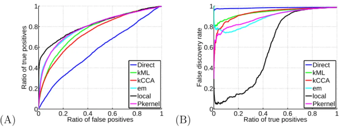
Figure 4: Performance of different methods for the reconstruction of the metabolic gene network from heterogeneous genomic datasets using the integrated kernel. (A) The ROC curves of the six methods, and (B) the FDR curve for the six methods. On this benchmark experiment, the local SVM method (“local”) can predict close to 45% of the correct edges with a false discovery rate smaller than 50%.
4
Results
We compared systematically all methods on both benchmark experiments. Results are summarized in Tables 1 and 2. We see in Table 1 that in terms of AUC, the local model performs on average as well as all of the non-Direct methods. In particular however, the local kernel gives the best AUC for the metabolic network integrated kernel, and gives a comparable result to the other methods for the protein-protein interaction integrated kernel. However, more importantly for practical applications, Table 2 shows the remarkable performance of the local method using the integrated kernel in terms of the FDR curve. This gain is further illustrated in Figure 6 for the metabolic network, and in Figure 7 for the protein-protein interaction network. Whilst indeed for each data set considered separately (“exp”, “loc” or “phy”), there is nothing particularly striking about the local method as compared to the others, the fact of summing these three data set’s kernels results in being able to correctly predict up to a total of 45% of the positive examples whilst maintaining an extremely small false discovery rate, as shown in Figure 4(B). This can incidentally be seen already in Figure 4(A) with the steep ascent of the local method’s ROC curve close to the origin. This is a surprisingly strong result. Perhaps for the first time for this metabolic network, an in silico method is powerful enough to have direct practical applications for biologists. Given an enzyme which is either newly discovered or for which the directly related enzymes are still undetermined, it follows that we can predict 45% of its directly related enzymes, for example 10 enzymes, and only make on average 10 mistaken other predictions. This is a magnitude of order time-saving with respect to having to consider literally hundreds of possibly related enzymes.
Figure 5(B) shows a similar result for the protein-protein interaction network, in that the local method using the integrated kernel significantly outperforms the other methods in terms of keeping a low false discovery rate with respect to the ratio of true positives, though this effect is less powerful than for the metabolic network. Indeed, as before, this result can be noticed directly via Figure 5(A) with the steep ascent of the local method ROC curve with respect to the other curves close to the origin.
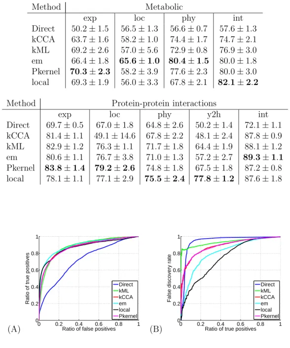
Table 1: Network reconstruction performance in terms of AUC. For each method (“Di-rect”: direct method; “kCCA”: kernel canonical correlation analysis method; “kML”: kernel met-ric learning method; “em”: em projection method; “Pkernel”: tensor product pairwise kernel with SVM; “local”: local models with SVM), we show the area under the ROC curve (AUC) estimated by 5-fold cross-validation on the reconstruction of the metabolic gene network and the protein-protein interaction network from different datasets (“exp”: expression data; “loc”: cellular localization; “phy”: phylogenetic profile; “int”: integration of the individual datasets).
Method Metabolic
exp loc phy int
Direct 50.2 ± 1.5 56.5 ± 1.3 56.6 ± 0.7 57.6 ± 1.3 kCCA 63.7 ± 1.6 58.2 ± 1.0 74.4 ± 1.7 74.7 ± 2.1 kML 69.2 ± 2.6 57.0 ± 5.6 72.9 ± 0.8 76.9 ± 3.0 em 66.4 ± 1.8 65.6 ± 1.0 80.4 ± 1.5 80.0 ± 1.8 Pkernel 70.3 ± 2.3 58.2 ± 3.9 77.6 ± 2.3 80.0 ± 3.0 local 69.3 ± 1.9 56.0 ± 3.3 67.8 ± 2.1 82.1 ± 2.2
Method Protein-protein interactions
exp loc phy y2h int
Direct 69.7 ± 0.5 67.0 ± 1.8 64.8 ± 2.6 50.2 ± 1.4 72.1 ± 1.1 kCCA 81.4 ± 1.1 49.1 ± 14.6 67.8 ± 2.2 48.1 ± 2.4 87.8 ± 0.9 kML 82.9 ± 1.2 76.3 ± 1.1 71.7 ± 1.8 64.4 ± 1.9 88.1 ± 1.2 em 80.6 ± 1.1 76.7 ± 3.8 71.0 ± 1.3 57.2 ± 2.7 89.3 ± 1.1 Pkernel 83.8 ± 1.4 79.2 ± 2.6 74.8 ± 1.8 67.5 ± 1.8 87.2 ± 0.8 local 78.1 ± 1.1 77.1 ± 2.9 75.5 ± 2.4 77.8 ± 1.2 87.6 ± 1.8 (A) 0 0.2 0.4 0.6 0.8 1 0 0.2 0.4 0.6 0.8 1
Ratio of false positives
Ratio of true positives
Direct kML kCCA em local Pkernel (B) 0 0.2 0.4 0.6 0.8 1 0 0.2 0.4 0.6 0.8 1
Ratio of true positives
False discovery rate
Direct kML kCCA em local Pkernel
Figure 5: Performance of different methods for the reconstruction of the protein-protein interaction network from heterogeneous genomic datasets using the integrated kernel. (A) The ROC curves of the six methods, and (B) the FDR curve for the six methods.
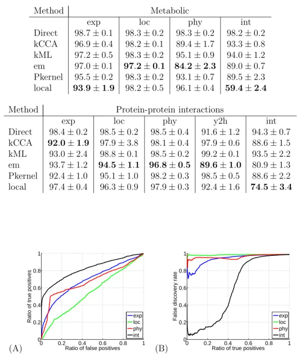
Table 2: Network reconstruction performance in terms of FDR. This table shows the performance of each method on each benchmark experiment in terms of area under the FDR curve.
Method Metabolic
exp loc phy int
Direct 98.7 ± 0.1 98.3 ± 0.2 98.3 ± 0.2 98.2 ± 0.2 kCCA 96.9 ± 0.4 98.2 ± 0.1 89.4 ± 1.7 93.3 ± 0.8 kML 97.2 ± 0.5 98.3 ± 0.2 95.1 ± 0.9 94.0 ± 1.2 em 97.0 ± 0.1 97.2 ± 0.1 84.2 ± 2.3 89.0 ± 0.7 Pkernel 95.5 ± 0.2 98.3 ± 0.2 93.1 ± 0.7 89.5 ± 2.3 local 93.9 ± 1.9 98.2 ± 0.5 96.1 ± 0.4 59.4 ± 2.4
Method Protein-protein interactions
exp loc phy y2h int
Direct 98.4 ± 0.2 98.5 ± 0.2 98.5 ± 0.4 91.6 ± 1.2 94.3 ± 0.7 kCCA 92.0 ± 1.9 97.9 ± 3.8 98.1 ± 0.4 97.9 ± 0.6 88.6 ± 1.5 kML 93.0 ± 2.4 98.8 ± 0.1 98.5 ± 0.2 99.2 ± 0.1 93.5 ± 2.2 em 93.7 ± 1.2 94.5 ± 1.1 96.8 ± 0.5 89.6 ± 1.0 80.9 ± 1.3 Pkernel 92.4 ± 1.0 95.1 ± 1.0 98.2 ± 0.3 98.5 ± 0.5 88.6 ± 2.2 local 97.4 ± 0.4 96.3 ± 0.9 97.9 ± 0.3 92.4 ± 1.6 74.5 ± 3.4 (A) 0 0.2 0.4 0.6 0.8 1 0 0.2 0.4 0.6 0.8 1
Ratio of false positives
Ratio of true positives
exp loc phy int (B) 0 0.2 0.4 0.6 0.8 1 0 0.2 0.4 0.6 0.8 1
Ratio of true positives
False discovery rate exp
loc phy int
Figure 6: Performance of the local SVM method with various datasets for the re-construction of the metabolic network. (A) The ROC curves, and (B) the FDR curves. Each curve corresponds to one dataset: “exp” = expression data, “loc”=cellular localization data, “phy”=phylogenetic profiles, “int”=integration of all data by summing the corresponding kernels. We note the dramatic improvement resulting from the integration of all data over each data taken individually.
(A) 0 0.2 0.4 0.6 0.8 1 0 0.2 0.4 0.6 0.8 1
Ratio of false positives
Ratio of true positives
exp loc phy y2h int (B) 0 0.2 0.4 0.6 0.8 1 0 0.2 0.4 0.6 0.8 1
Ratio of true positives
False discovery rate
exp loc phy y2h int
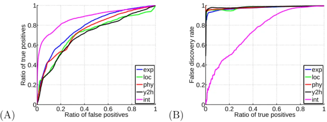
Figure 7: Performance of the local SVM method with various datasets for the recon-struction of the protein-protein interaction network. (A) The ROC curves, and (B) the FDR curves. Each curve corresponds to one dataset. “exp”, “loc”, “phy” and “y2h” correspond respectively to gene expression, cellular localization, phylogenetic profiles, and yeast 2-hybrid data. “int” corresponds to the integration of all data.
5
Discussion
We have proposed a conceptually simple approach for supervised graph reconstruction, based on learning independent local models to predict which new vertices are connected to each node in the training set. Immediately we can perceive some advantages and disadvantages of this method. In terms of advantages, this algorithm leaves the user entirely free to choose a class of classification rules and the criteria used for choosing a specific rule from that class. This means that any useful prior knowledge can be implemented into the classification task. However here, in order to more easily directly compare results, we used the kernels created in [27] and [11]. Therefore, there is indeed strong potential that the local method could perform even better given more pertinent kernel matrices.
We note also that the local method potentially has a de-noising capacity in that a classification rule is specifically used for each vertex of the graph G, so no effects from choosing the “averagely best rule” over the whole graph are encountered. This means that an optimum performance of the combined set of chosen rules is achieved over the whole graph, which is not necessarily the case for a global method. Furthermore, it is easy to envision an extension where the graph G is only partially known, that is, when instead of knowing whether or not there is an edge between every pair of vertices, we only know this for some pairs of vertices but not all. By using the parts of the graph we do know to select rules, vertex by vertex, with this method, we can then apply these rules to predict the existence or absence of the unknown edges between these same vertices of the graph G.
Another potential advantage of the local approach is that it straightforwardly extends to the inference of directed graphs, that are more natural representations of regulatory or signaling path-ways than undirected graphs, in particular. Indeed one could proceed by training two SVM for each node, one to identify the vertices pointed by and the other to identify the vertices pointing to the local node. Combined with the fact that the training of a local SVM only requires a descrip-tion of the local subnetworks suggest a variety of promising applicadescrip-tions, e.g., the identificadescrip-tion of genes regulated by a transcription factor of interest.
Specifically, if we instead have two new vertices Xk1 and Xk2, we cannot immediately predict
whether there is an edge between them. However, if the number of new vertices is small with respect to the number of vertices of G, this is not such a large problem in terms of the percentage of the whole graph (G plus the new vertices and edges) we can predict. In any case, possible solutions include (for biological graphs) experimentally verifying the existence or absence of the remaining edges in vivo, or (for any type of graph) relating one of two new vertices to the closest vertex Xi of G (under some metric) and then stealing the classification rule related to Xi. The
development of this type of solution is beyond the scope of the present paper, and will depend in particular on the class of classification rules implemented by the user.
We emphasise again that data integration via the simple addition of different kernels had a remarkable effect on improving the performance of the local method. Whilst this kind of improve-ment has been seen before to a small extent, in the present case the results were startling. Further improvement might be possible by replacing the simple sum of kernels by, e.g., weighted sums, building on recent works an the problem of learning from multiple kernels [13].
Taking into account the strong performance of the local method with the integrated kernel, as seen in the FDR curves, especially for the metabolic network, it now seems possible that these results can be directly applied to real present biological problems such as finding missing enzymes or predicting new pathways. In the metabolic network for example, there are more than 220 000 pairs of enzymes for which no direct functional relationship is known. It would seem very likely that some of these are in fact directly related enzymes, yet have never been experimentally found to be such. Using the local method results, it would therefore seem like a good strategy to take pairs of enzymes which were very strongly predicted to be directly related, but for which no direct relationship is yet known, and to test if they are related by lab experiments. We intend to proceed with an explicit enumeration of these predictions and experimental validation in future work.
Due to these improved developments in prediction accuracy for at least up to 50% of the true positively labelled examples (which is furthermore remarkable in the sense that the number of negative examples vastly outweighs the number of postive examples), we wonder whether the FDR curve is not a more pertinent performance measure than the AUC value for extremely unbalanced (positive versus negative examples) problems. Indeed, what is at present critical in ROC curves is the behaviour of the curve close to the origin, rather than precisely the AUC value. For the present benchmark data sets (which are extremely unbalanced), as the goal is indeed practical biological applications, an ROC curve which rises steeply close to the origin but then performs poorly far from the origin is in a sense better than an ROC curve which does exactly the opposite, even if this curve has a higher AUC value. We suggest that in future work on such unbalanced problems, the FDR curve must also play an important role in the evaluation of new methods, and not only the AUC value.
Acknowledgement
We thank T. Kato and Y. Yamanishi for making their data public. We also thank G. Loosli and A. Rakotomamonjy for help with the use of simpleSVM. K. B. is the recipient of a doctoral grant from the Minist`ere de l’Education Nationale, de l’Enseignement Sup´erieur et de la Recherche (MENESR) Universit´e Montpellier II. G. B. is supported by the Institut de Math´ematiques et de Mod´elisation de Montpellier (Universit´e Montpellier II, UMR CNRS 5149). J.-P. V. is supported by National Institute of Health award NHGRI R33 HG003070, by the French Ministry for Research and New Technologies grant ACI-IMPBIO-2004-47, and by the EC contract ESBIC-D
(LSHG-CT-2005-518192).
References
[1] A. Ben-Hur and W. S. Noble. Kernel methods for predicting protein-protein interactions. Bioinformatics, 21(Suppl. 1):i38–i46, Jun 2005.
[2] G. Biau and K. Bleakley. Statistical inference on graphs. Statistics and Decisions, 24(2):209– 232, 2006.
[3] A. Doi, H. Matsuno, M. Nagasaki, and S. Miyano. Hybrid Petri net representation of gene regulatory network. In Proceedings of the Pacific Symposium on Biocomputing, volume 5, pages 341–352, 2000.
[4] M. B. Eisen, P. T. Spellman, P. O. Brown, and D. Botstein. Cluster analysis and display of genome-wide expression patterns. Proc. Natl. Acad. Sci. USA, 95:14863–14868, Dec 1998. [5] N. Friedman, M. Linial, I. Nachman, and D. Pe’er. Using Bayesian networks to analyze
expression data. J. Comput. Biol., 7(3-4):601–620, 2000.
[6] W.-K. Huh, J. V. Falvo, L. C. Gerke, A. S. Carroll, R. W. Howson, J. S. Weissman, and E. K. O’Shea. Global analysis of protein localization in budding yeast. Nature, 425(6959):686–691, Oct 2003.
[7] T. Ito, T. Chiba, R. Ozawa, M. Yoshida, M. Hattori, and Y. Sakaki. A comprehensive two-hybrid analysis to explore the yeast protein interactome. Proc. Natl. Acad. Sci. USA, 98(8):4569–4574, 2001.
[8] R. Jansen, H. Yu, D. Greenbaum, Y. Kluger, N. J. Krogan, S. Chung, A. Emili, M. Snyder, J. F. Greenblatt, and M. Gerstein. A Bayesian networks approach for predicting protein-protein interactions from genomic data. Science, 302(5644):449–453, 2003.
[9] M. Kanehisa. Prediction of higher order functional networks from genomic data. Pharma-cogenomics, 2(4):373–385, 2001.
[10] M. Kanehisa, S. Goto, S. Kawashima, Y. Okuno, and M. Hattori. The KEGG resource for deciphering the genome. Nucleic Acids Res., 32(Database issue):D277–80, Jan 2004.
[11] T. Kato, K. Tsuda, and K. Asai. Selective integration of multiple biological data for supervised network inference. Bioinformatics, 21(10):2488–2495, May 2005.
[12] R. I. Kondor and J. Lafferty. Diffusion Kernels on Graphs and Other Discrete Input. In ICML 2002, 2002.
[13] G. R. G. Lanckriet, T. De Bie, N. Cristianini, M. I. Jordan, and W. S. Noble. A statistical framework for genomic data fusion. Bioinformatics, 20(16):2626–2635, 2004.
[14] G. Loosli. Simplesvm toolbox. Available at http://asi.insa-rouen.fr/ gloosli/simpleSVM.html, 2006.
[15] E.M. Marcotte, M. Pellegrini, H.-L. Ng, D.W. Rice, T.O. Yeates, and D. Eisenberg. Detecting Protein Function and Protein-Protein Interactions from Genome Sequences. Science, 285:751– 753, 1999.
[16] P. Pavlidis, J. Weston, J. Cai, and W.S. Noble. Learning Gene Functional Classifications from Multiple Data Types. J. Comput. Biol., 9(2):401–411, 2002.
[17] F. Pazos and A. Valencia. Similarity of phylogenetic trees as indicator of protein-protein interaction. Protein Eng., 9(14):609–614, 2001.
[18] B. Sch¨olkopf and A. J. Smola. Learning with Kernels: Support Vector Machines, Regulariza-tion, OptimizaRegulariza-tion, and Beyond. MIT Press, Cambridge, MA, 2002.
[19] B. Sch¨olkopf, K. Tsuda, and J.-P. Vert. Kernel Methods in Computational Biology. MIT Press, 2004.
[20] P. T. Spellman, G. Sherlock, M. Q. Zhang, V. R. Iyer, K. Anders, M. B. Eisen, P. O. Brown, D. Botstein, and B. Futcher. Comprehensive identification of cell cycle-regulated cenes of the yeast Saccharomyces cerevisiae by microarray hybridization. Mol. Biol. Cell, 9:3273–3297, 1998.
[21] K. Tsuda, S. Akaho, and K. Asai. The em algorithm for kernel matrix completion with auxiliary data. J. Mach. Learn. Res., 4:67–81, 2003.
[22] Peter Uetz, Loic Giot, Gerard Cagney, Traci A. Mansfield, Richard S. Judson, James R. Knight, Daniel Lockshon, Vaibhav Narayan, Maithreyan Srinivasan, Pascale Pochart, Alia Qureshi-Emili, Ying Li, Brian Godwin, Diana Conover, Theodore Kalbfleish, Govindan Vi-jayadamodar, Meijia Yang, Mark Johnston, Stanley Fields, and Jonathan M. Rothberg. A comprehensive analysis of protein-protein interactions in Saccharomyces cerevisiae. Nature, 403:623–627, 2000.
[23] V. N. Vapnik. Statistical Learning Theory. Wiley, New-York, 1998.
[24] J.-P. Vert and Y. Yamanishi. Supervised graph inference. In Lawrence K. Saul, Yair Weiss, and L´eon Bottou, editors, Adv. Neural Inform. Process. Syst., volume 17, pages 1433–1440. MIT Press, Cambridge, MA, 2005.
[25] C. von Mering, R. Krause, B. Snel, M. Cornell, S. G. Oliver, S. Fields, and P. Bork. Compara-tive assessment of large-scale data sets of protein-protein interactions. Nature, 417(6887):399– 403, May 2002.
[26] Y. Yamanishi, J.-P. Vert, and M. Kanehisa. Protein network inference from multiple genomic data: a supervised approach. Bioinformatics, 20:i363–i370, 2004.
[27] Y. Yamanishi, J.-P. Vert, and M. Kanehisa. Supervised enzyme network inference from the integration of genomic data and chemical information. Bioinformatics, 21:i468–i477, 2005.
![Figure 1: Part of the aminosugars metabolic network, which can be extracted from the KEGG database [10].](https://thumb-eu.123doks.com/thumbv2/123doknet/8223379.276461/4.918.284.636.81.430/figure-aminosugars-metabolic-network-extracted-kegg-database.webp)