HAL Id: hal-00666143
https://hal.archives-ouvertes.fr/hal-00666143
Submitted on 3 Feb 2012
HAL is a multi-disciplinary open access
archive for the deposit and dissemination of
sci-entific research documents, whether they are
pub-lished or not. The documents may come from
teaching and research institutions in France or
abroad, or from public or private research centers.
L’archive ouverte pluridisciplinaire HAL, est
destinée au dépôt et à la diffusion de documents
scientifiques de niveau recherche, publiés ou non,
émanant des établissements d’enseignement et de
recherche français ou étrangers, des laboratoires
publics ou privés.
images
Tarik Filali Ansary, Jean-Philippe Vandeborre, Mohamed Daoudi
To cite this version:
Tarik Filali Ansary, Jean-Philippe Vandeborre, Mohamed Daoudi. A framework for 3D CAD models
retrieval from 2D images. Annals of Telecommunications - annales des télécommunications, Springer,
2005, 60 (11-12), pp.1337-1359. �hal-00666143�
from 2D images.
Un cadre pour l’indexation de modèles 3D
CAO à partir d’images 2D.
Tarik Filali Ansary, Jean-Philippe Vandeborre, Mohamed Daoudi
Equipe FOX-MIIRE − LIFL (UMR USTL-CNRS 8022)
GET / INT / ENIC Télécom Lille 1, rue G. Marconi, cité scientifique
59658 Villeneuve d’Ascq cedex, France
{filali, vandeborre, daoudi}@enic.fr
RÉSUMÉ. La gestion de grandes bases de données de modèles tridimensionnels (utilisés dans des applications de CAO, de visualisation, des jeux, etc.) est un domaine très important. La capacité de caractériser et rechercher facilement des modèles est une question clé pour les concepteurs et les utilisateurs finaux. Deux approches principales existent : la recherche par l’exemple d'un modèle tridimensionnel, et la recherche par une vue 2D ou des photos. Dans cet article, nous présentons un cadre pour la caractérisation d'un modèle 3D par un ensemble de vues (appelées vues caractéristiques), et un processus d'indexation de ces mo-dèles avec une approche probabiliste bayésienne en utilisant les vues caractéristiques. Le système est indépendant du descripteur utilisé pour l'indexation. Nous illustrons nos résultats en utilisant différents descripteurs sur une collection de modèles tridimensionnels fournis par le constructeur automobile Renault. Nous présentons également nos résultats sur l’indexa-tion de modèle 3D à partir de photos.
ABSTRACT. The management of big databases of three-dimensional models (used in CAD applications, visualisation, games, etc.) is a very important domain. The ability to characterise and easily retrieve models is a key issue for the designers and the final users. In this frame, two main approaches exist: search by example of a three-dimensional model, and search by a 2D view or photos. In this paper, we present a novel framework for the characterisation of a 3D model by a set of views (called characteristic views), and an indexing process of these models with a Bayesian probabilistic approach using the characteristic views. The framework is independent from the descriptor used for the indexing. We illustrate our results using different descriptors on a collection of three-dimensional models supplied by the car manufacturer Renault. We also present our results on retrieval of 3D models from a single photo.
MOTS-CLÉS : modèles 3D, vues caractéristiques, indexation, photos.
I. Introduction
The use of three-dimensional images and models databases through the Internet is growing both in number and in size. The development of modelling tools, 3D scanners, 3D graphic accelerated hardware, Web3D and so on, is enabling access to three-dimensional materials of high quality. In recent years, many systems have been proposed for efficient information retrieval from digital collections of images and videos.
The SEMANTIC-3D1 project aims the exploration of techniques and tools preliminary to the realisation of new services for the exploitation of 3D contents through the Web. New techniques of compression, indexing and watermarking of 3D data will be developed and implemented in a industrial prototype application: a communication and information system (consultation, remote support) between the authors (originators of machine elements), users (car technician) and a central server of 3D data. The compressed 3D data exchanges adapt to the rate of transmission and the capacity of the terminals used.
These exchanges are ensured with a format of data standardised with functionalities of visualisation and 3D animation. The exchanges are done on existing networks (internal network for the authors, wireless networks for the technicians).
In SEMANTIC-3D project, our research group focuses on the indexing and retrieval of 3D data. The solutions proposed so far to support retrieval of such data are not always effective in application contexts where the information is intrinsically three-dimensional. A similarity metric has to be defined to compute a visual similarity between two 3D models, given their descriptions. Two families of methods for 3D models retrieval exist: 3D/3D (direct model analysis) and 2D/3D (3D model analysis from its 2D views or photos) retrieval.
For example, Vandeborre et al. [1] propose to use full three-dimensional information. The 3D objects are represented as mesh surfaces and 3D shape descriptors are used. The results obtained show the limitation of the approach when the mesh is not regular. This kind of approach is not robust in terms of shape representation.
Sundar et al. [2] intend to encode a 3D object in the form of a skeletal graph. They use graph matching techniques to match the skeletons and, consequently, to compare the 3D objects. They also suggest that this skeletal matching approach has the ability to achieve part-matching and helps in defining the queries instinctively.
In 2D/3D retrieval approach, two serious problems arise: how to characterise a 3D model with few 2D views, and how to use these views to retrieve the model from a 3D models collection.
Abbasi and Mokhtarian [3] propose a method that eliminates the similar views in the sense of a distance among CSS (Curvature Scale Space) from the outlines of these views. At last, the minimal number of views is selected with an optimisation algorithm.
1
Dorai and Jain [4] use, for each of the model in the collection, an algorithm to generate 320 views. Then, a hierarchical classification, based on a distance measure between curvatures histogram from the views, follows.
Mahmoudi and Daoudi [5] also suggest to use the CSS from the outlines of the 3D model extracted views. The CSS is then organised in a tree structure called
M-tree.
Chen and Stockman [6] as well as Yi and al. [7] propose a method based on a bayesian probabilistic approach. It means computing an a posteriori probability to recognise the model when a certain feature is observed. This probabilistic method gives good results, but the method was tested on a small collection of 20 models.
Chen et al. [8][9] defend the intuitive idea that two 3D models are similar if they also look similar from different angles. Therefore, they use 100 orthogonal projections of an object and encode them by Zernike moments and Fourier descriptors. They also point out that they obtain better results than other well-known descriptors as the MPEG-7 3D Shape Descriptor.
Ohbuchi and Nakazawa [10] propose a brute force appearance based method. The approach is based on the comparison of 42 depth images created from each model.
Costa and Shapiro [11] propose a Relational Indexing of Objects (RIO) recognition system. The performance on CAD database was very good with the exception of a few misdetection cases. However these results are given for a very small database (five 3D objects).
For a more complete state of the art, Tangelder and Veltkamp [12] gives a survey of recent methods for content based 3D shapes retrieval.
In this paper, we propose a framework for 3D models indexing based on 2D views. The goal of this framework is to provide a method for optimal selection of 2D views from a 3D model, and a probabilistic Bayesian method for 3D models indexing from these views. The framework is totally independent from the 2D view descriptor used, but the 2D view descriptors should provide some properties. The entire framework has been tested with three different 2D descriptors.
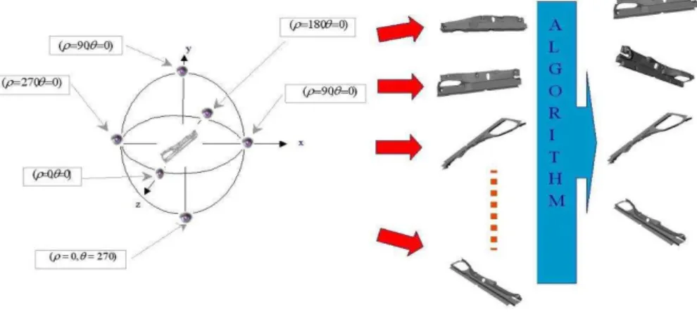
Figure 1 shows an overview of the system. The offline process of characteristic view selection and the online process of retrieval using bayesian approach.
This paper is organised in the following way. In section 2 and 3, we present the main principles of our framework for characteristic views selection and probabilistic 3D models indexing. In section 4, three different 2D view descriptors are explained in details. Finally, the results obtained from a collection of 3D models are presented for each 2D view descriptor showing the performances of our framework.
II. Characteristic views algorithm
In this paragraph, we present our algorithm for optimal characteristic views selection from a three-dimensional model.
Let Db = {M1, M2, …, MN} be a collection of N three-dimensional models. We
wish to represent each 3D model Mi by a set of 2D views that represent it the best.
To achieve this goal, we first generate an initial set of views from the 3D model, then we reduce it to the only views that characterise best the 3D model. This idea come from the fact that not all the views of 3D model got equal importance, there are views that contain more information than others.
Figure 2 shows an overview of the characteristic views selection process
Figure 2. Characteristic views selection process. Processus de choix des vues caractéristiques.
II.1. Generating the initial set of views
To generate the initial set of views for a model Mi of the collection, we create
2D views (projections) from multiple viewpoints. These viewpoints are equally spaced on the unit sphere. In our current implementation, there are 80 views. In fact, we scale each of our model that it can fit in a unit sphere and we translate it, that the origin coincide with the 3D model barycenter.
To select positions for the views, that must be equally spaced, we use a two units icosahedron centred on the origin. We subdivide the icosahedron once by using the Loop's subdivision scheme to obtain an 80 faceted polyhedron. Finally to generate the initial views we place the camera on each of the face-center of the polyhedron looking at the coordinate origin.
II.2. Discrimination of characteristic views
Let VM ={VM1,VM2,...,VMv} be the set of 2D views from the three-dimensional model M, where v is the total number of views.
Among this set of views, we have to select those that characterise effectively the three-dimensional model according to a feature of these views.
II.3. Selection of characteristic views
The next step is to reduce the set of views of a model M to a set that represents only the most important views. This set is called the set of characteristic views VcM.
A view
V
Mk is a characteristic view of a model M for a distance ε, if the distance between this view and all the other characteristic views of M is greater thanε. That is to say:
ε
>
∈
∀
⇔
∈
k M j M M M V Vc k M M jD
Vc
Vc
Vc
V
,
, With k M j M Vc VD
, the distance between the descriptor of the view
j M
V
and the descriptor ofVc
Mk .However, the choice of the distance threshold ε is important and depends on the complexity of the three-dimensional model. This information is not a priori known.
To solve the problem of determining the distance threshold ε, we adapted the previous algorithm by taking into account an interval of these distances from 0 to 1 with a step of 0.001. The final set of characteristic views is then the union of all the sets of characteristic views for every ε in ]0..1[.
It means that, we consider a view to be important if it belongs frequently to the sets of characteristic views for different ε. So the final set of characteristic views for a 3D model is then the set of views that are frequently considered as characteristic.
Figure 3. An example of characteristic views for a cube. Un exemple de vues caractéristiques pour un cube.
II.4 Properties of the views selection algorithm
To reduce the number of characteristic views, we filter this set of views in a way that for each model it verifies two criterions:
- Each view of the model M must be represented by at least one characteristic view for every threshold ε . This mean that, if we assume that our algorithm is a function
ℜ
between the initial set and the characteristic set, this functionℜ
must be an application associating to each element of VMat least oneelements of VcM: k M M j M
V
Vc
V
∈
∃
∀
,
such asℜ
(
V
Mj)
=
Vc
Mk- Now that we are sure that every initial view got a characteristic view representing it, we want our set to be composed with the minimum of characteristic views that respect the first property. This means that we do not want any redundant characteristic view.
Let
Vr
Mj be the set of views represented by the characteristic viewVc
Mj . A characteristic viewVc
Mj is redundant if there is a set of characteristic views for which the union of represented views includesVr
Mj .⊂
j MVr
k MVr
U
The following algorithm (see next page) summarizes the characteristic view selection process:
Characteristic views selection algorithm For
α
from 0 to 1 doSelect characteristic views for the threshold
ε
;
Reduce the views to the minimum necessary with respect to the property of representation ;
Save the characteristic view set ;
Done ;
For all views do
Compute how many times the view is selected as a characteristic view ;
Done ;
Select the most frequently chosen views as characteristic views.
III. Probabilistic approach for 3D indexing
Each model of the collection Db is represented by a set of characteristic views
}
Vc
,...,
Vc
,
{Vc
1 2 vˆ=
CV
, withvˆ
the number of characteristic views. To each characteristic view corresponds a set of represented views calledVr.Considering a 2D request view Q, we wish to find the model
M
i∈
D
b which one of its characteristic views is the closest to the request view Q. This model is the one that has the highest probabilityP(M ,Vcj /Q)M i
i
.
Let H be the set of all the possible hypotheses of correspondence between the request view Q and a model M,
H
=
{
h
1∨
h
2∨
...
∨
h
vˆ}
. A hypothesisk
h
means that the view k of the model is the view request Q. The sign∨
representslogic or operator. Let us note that if an hypothesis
h
k is true, all the other hypo-theses are false.) Q / Vc , M ( P j M i i can be expressed by P(M ,Vcj /H) M i i .
The closest model is the one that contains a view having the highest probability. Using the Bayes theorem, we have:
)
(
)
/
,
(
)
,
,
(
j i i M j M iH
Vc
P
H
Vc
M
P
M
M
P
i i=
(1))
(
)
/
,
(
)
,
,
(
M
H
Vc
P
M
Vc
H
P
H
P
i Mj j M i i=
i (2)From (1) and (2), we have:
)
(
)
(
)
/
,
(
)
/
,
(
H
P
M
P
M
Vc
H
P
H
Vc
M
P
i i j M j M i i i=
(3)We also have:
∑
= = v k i j M k i j M M P h Vc M Vc H P i i ˆ 1 ) / , ( ) / , ( (4)This probability will be equal to zero for every k different from j, because we assume that a view cannot look like to characteristic views at the same time (our algorithm for view selection would have detect it, and deleted one of the views). The sum
∑
= v k i j M k Vc M h P i ˆ 1 ) / ,( can be reduced to the only true hypothesis
)
/
,
(
h
jVc
MjM
iP
i .By integrating this remark to (4) , we obtain:
)
/
,
(
)
/
,
(
j i M j i j MM
P
h
Vc
M
Vc
H
P
i i=
and)
/
(
)
,
/
(
)
/
,
(
j i M i j M j i j M jVc
M
P
h
Vc
M
P
Vc
M
h
P
i i i=
(4’)From (3) and (4’), we obtain:
)
(
)
(
)
/
(
)
,
/
(
)
/
,
(
H
P
M
P
M
Vc
P
M
Vc
h
P
H
Vc
M
P
i i j M i j M j j M i i i i=
(5) We also have:)
(
)
/
(
)
,
/
(
)
,
,
(
)
(
1 ˆ 1 1 ˆ 1∑∑
∑∑
= = = ==
=
N i v j N i v j i i j M i j M j j M iV
P
h
Vc
M
P
Vc
M
P
M
M
H
P
H
P
i i i (6) Finally from (5) et (6), we get:∑∑
= ==
N i v j i i j M i j M j i i j M i j M j j M iM
P
M
Vc
P
M
Vc
h
P
M
P
M
Vc
P
M
Vc
h
P
H
Vc
M
P
i i i i i 1 ˆ 1)
(
)
/
(
)
,
/
(
)
(
)
/
(
)
,
/
(
)
/
,
(
With P(Mi) the probability to observe the model Mi.
∑
= − −=
N i Vc N Vc N Vc N Vc N i Mi i Me
e
M
P
1 ) ( ) ( ) ( ) ()
(
α α Where(
)
i MVc
N
is the number of characteristic views of the model Mi, andN(Vc) is the total number of characteristic views for the set of the models of the collection Db. α is a parameter to hold the effect of the probability P(Mi). The algorithm conception makes that, the greater the number of characteristic views of an object, the more it is complex. Indeed, simple object (e.g. a cube) can be at the root of more complex objects.
On the other hand:
(
)
(
)
∑
= − ⋅ ⋅ −−
−
=
N j Vr N Vr N Vr N Vr N i j M i M j Mi i M j Mi ie
e
M
Vc
P
1 ) ( ) ( ) ( ) ()
1
(
1
)
/
(
β ββ
β
Where ( ) j Mi VrN is the number of views represented by the characteristic view
j Mi
Vc
of the model Mi, and N(VrMi) is the total number of views represented by themodel Mi. Coefficient β is introduced to reduce the effect of the view probability. We use the values α =β= 1/100 which give the best results during our experiments. The greater is the number of represented views N(VrMij ) , the more the characteristic view VcMij is important and the best it represents the three-dimensional model. The value
(
/
,
i)
j M jVc
M
h
P
i is the probability that, knowing that we observe
the characteristic view j of the model
M
i , this view is the request view Q:∑
= − −=
N j Vc Q D Vc Q D i j M j j i M j i M ie
e
M
Vc
h
P
1 ) , ( ) , ()
,
/
(
With ( , ) j i M Vc QD the distance between the 2D descriptors of Q and of the
j Mi
Vc
characteristic view of the three-dimensional model Mi.IV. Shape descriptors used for a view
As mentioned before, the framework we describe in this paper is independent from the 2D descriptor used, but, to use a descriptor within our framework some properties are required. The descriptor used must be:
1) Invariance: the shape descriptors must be independent of the group of similarity transformation (the composition of a translation, a rotation and a scale factor).
2) Stability gives robustness under a small distortions caused by a noise and non-linear deformation of the object.
3) Simplicity and real time computation.
To test our framework with different types of descriptors, we implemented our system with three different descriptors that are well known as efficient methods for a global a shape representation:
1) the curvatures histogram [13]; 2) the Zernike moments [17];
IV.1. Curvatures histogram
The curvatures histogram is based on shape descriptor, named curvature index, introduced by Koenderink and Van Doorn [13]. This descriptor aims at providing an intrinsic shape descriptor of three-dimensional mesh-models. It exploits some local attributes of a three-dimensional surface. The curvature index is defined as a function of the two principal curvatures of the surface. This three-dimensional shape index was particularly used for the indexing process of fixed images [14], depth images [4], and three-dimensional models [1][15].
Computation of the curvatures histogram for a 2D view
To use this descriptor with our 2D views, a 2D view needs to be transformed in the following manner. First of all, the 2D view is converted into a gray-level image. The Z coordinate of the points is then equal to the gray-intensity of the considered pixel (x,y,I(x,y)) to obtain a three-dimensional surface in which every pixel is a point of the surface. Hence, the 2D view is equivalent to a three-dimensional terrain on which a 3D descriptor can be computed.
Let p be a point on the three-dimensional terrain. Let us denote by k1and k2the principal curvatures associated with the point p. The curvature index value at this point is defined as:
2 1 2 1 p k k k k arctan 2 I − + π = with k
1
≥k2
The curvature index value belongs to the interval [-1, +1] and is not defined for planar surfaces. The curvature histogram of a 2D view is then the histogram of the curvature values calculated over the entire three-dimensional terrain.
Figure 4 shows the curvatures histogram for a view of one of our 3D models.
Figure 4. Curvatures histogram of a 2D view. Histogramme de courbures d'une vue 2D .
Comparison of views described by the curvature histogram
Each view is then described with its curvatures histogram. To compare two views, it is enough to compare their respective histograms. There are several ways to compare distribution histograms: the Minkowski Ln norms,
Kolmogorov-Smirnov distance, Match distances, and many others. We choose to use the L1 norm
because of its simplicity and its accurate results.
)
(
)
,
(
1 2 1 2 1∫
+∞ ∞ −−
=
f
f
f
f
D
LThe calculation of the distance between the histograms of two views can be then considered as the distance between these views.
IV.2. Zernike moments
Zernike moments are complex orthogonal moments whose magnitude has rotational invariant property. Zernike moments are defined inside the unit circle, and the orthogonal radial polynomial
ℜ
nm(
P
)
is defined as:∑
− = − − − + − − = ℜ ( )/2 0 2 ! 2 ! 2 ! )! ( ) 1 ( ) ( m n s s n s nm p m n s m n s s n Pwhere n is a non-negative integer, and m is a non-zero integer subject to the following constraints:
n
−
m
is even andm
≤
n
. The (n,m) of the Zernike basis function,V
nm(
ρ
,
θ
)
, defined over the unit disk is:1 ), exp( ) ( ) , (
ρ
θ
=ℜ P jmθ
ρ
≤ Vnm nmThe Zernike moment of an image is then defined as:
)
,
(
)
,
(
1
*ρ
θ
ρ
θ
π
V
f
n
Z
disk unit nm nm∫∫
+
=
where
V
nm* is a complex conjugate ofV
nm. Zernike moments have the following properties: the magnitude of Zernike moment is rotational invariant; they are robust to noise and minor variations in shape; there is no information redundancy because the bases are orthogonal.An image can be better described by a small set of its Zernike moments than any other type of moments such as geometric moments, Legendre moments, rotational moments, and complex moments in terms of mean-square error; a relatively small set of Zernike moments can characterise the global shape of a pattern effectively, lower order moments represent the global shape of a pattern and higher order moments represent the detail.
The defined features on the Zernike moments are only rotation invariant. To obtain scale and translation invariance, the image is first subject to a normalisation process. The rotation invariant Zernike features are then extracted from the scale and translation normalised image. Scale invariance is accomplished by enlarging or reducing each shape such that its zeroth order moment m00 is set equal to a predetermined value β. Translation invariance is achieved by moving the origin to
the centroid before moment calculation. In summary, an image function f(x,y) can be normalised with respect to scale and translation by transforming it into g(x,y) where:
) / , / ( ) , (x y f x a x y a y g = + +
with
(
x
,
y
)
being the centroid of f(x,y) and00
/ m
a=
β
. Note that in the case of binary image m00is the total number of shape pixels in the image.To obtain translation invariance, it is necessary to know the centroid of the object in the image. In our system it is easy to achieve translation invariance, because we use binary images, the object in each image is assumed to be composed by black pixels and the background pixels are white.
In our current system, we extracted Zernike features starting from the second order moments. We extract up to twelfth order Zernike moments corresponding to 47 features. The detailed description of Zernike moments can be found in [16][19].
IV.3. Curvature Scale Space
Assuming that each image is described by its contour, the representation of image curves γ, which correspond to the contours of objects, are described as they appear in the image [17][18]. The curve γ is parameterised by the arc-length parameter. It is well known that there are different curve parameterisation to represent a given curve. The normalised arc-length parameterisation is generally used when the invariance under similarities of the descriptors is required. Let γ(u) be a parameterised curve by arc-length, which is defined by γ = {(x(u), y(u)| u ∈ [0,1]}. An evolved γσ version of γ {γσ | σ ≥ 0} can be computed. This is defined by:
γσ =
{
x(
u,σ) (
,y u,σ)
u∈[ ]
0,1}
where,( ) ( ) ( )
u
,
σ
=
x
u
*
g
u
,
σ
x
( ) ( ) ( )
u
,
σ
=
y
u
*
g
u
,
σ
y
with ∗ being the convolution operator and g(u,σ) a Gaussian width σ. It can be shown that curvature k on γσ is given by:
3/2 2 u 2 u u uu uu u
)
)
(u,
y
)
(u,
(x
)
(u,
y
)
(u,
x
-)
(u,
y
)
(u,
x
)
k(u,
σ
+
σ
σ
σ
σ
σ
=
σ
Thecurvature scale space (CSS) of the curve γ is defined as a solution to:
( )
u, 0 k σ =The curvature extrema and zeros are often used as breakpoints for segmenting the curve into sections corresponding to shape primitives. The zeros of curvature are points of inflection between positive and negative curvatures. Simply the breaking of every zero of curvature provides the simplest primitives, namely convex and concave sections. The curvature extrema characterise the shape of these sections.
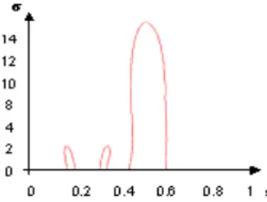
Figure 6 shows the CSS image corresponding to the contour of an image corresponding to a view of a 3D model (figure 5).
The X and Y axis respectively represent the normalised arc length (u) and the standard deviation (σ). Since now, we will use this representation. The small peaks on CSS represent noise in the contour. For each σ, we represented the values of the various arc length corresponding to the various zero crossing. On the Figure 4, we notice that for σ=12 the curve has 2 zero-crossing. So we can note that the number of inflection point decrease when non convex curve converges towards a convex curve.
The CSS representation has some properties as:
- The CSS representation is invariant under the similarity group (the composition of a translation, a rotation, and a scale factor).
- Completeness: This property ensures that two contours will have the same shape if and only if all their CSS are equal.
- Stability gives robustness under small distortions caused by quantisation. - Simplicity and real time computation. This property is very important in database applications.
Figure 5. Contour corresponding to a view of a 3D model from the collection. Contour correspondant à une vue d'un modèle 3D de la collection.
Figure 6. Curvature Scale Space corresponding to figure 5. Curvature Scale Space correspondant à la figure 5.
In order to compare the index based on CSS, we used the geodesic distance defined in [20]. Given two points (s1,σ1) and (s2,σ2), with σ1<σ2, their distance D can be defined in the following way:
(
) (
)
(
)
( )
( )
− + − + − = L s s D ϕ ϕσ ϕσ σ σ σ σ 2 1 2 1 1 2 2 2 1 1 1 1 1 1 log , , , where :(
)
(
(
2)
)
2 2 1 2 2 2 2 2 2 1 2 2 σ σ σ σ ϕ + + + − = L L Land
L
=
s
1−
s
2 is the Euclidean distance.V. Experiences and results
We implemented the algorithms, described in the previous sections, using C++ and the TGS OpenInventor.
To measure the performance, we classified the 760 models of our collection into 76 classes based on the judgement of the SEMANTIC project members (figure 7).
We used several different performance measures to objectively evaluate our method: the First Tier (FT), the Second Tier (ST), and Nearest Neighbor (NN) match percentages, as well as the recall-precision plot.
Recall and precision are well known in the literature of content-based search and retrieval. The recall and precision are defined as follows:
Recall = N/Q, Precision = N/A
With N the number of relevant models retrieved in the top A retrievals. Q is the number of relevant models in the collection, that are, the class number of models to which the query belongs to.
FT, ST, and NN percentages are defined as follows. Assume that the query belongs to the class C containing Q models. The FT percentage is the percentage of the models from the class C that appeared in the top (Q-1) matches.
The ST percentage is similar to FT, except that it is the percentage of the models from the class C the top 2(Q-1) matches. The NN percentage is the percentage of the cases in which the top matches are drawn from the class C.
We test the performance of our method with and without the use of the probabilistic approach. To produce results, we queried a random model from each class. Five random views were taken form every selected model. Results are the average of 70 queries.
As mentioned before, we used three different descriptors in our probabilistic framework.
V.1. Curvatures histogram
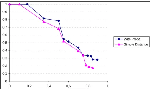
The main problem with the curvature histogram is its dependency on the light position. A small change in the lightening make changes in the curvature, that leads to a difference in the curvature histogram. In our tests, we are controlling the light position, but in real use conditions, this constraint can be very hard to obtain for the user. Table 1 shows performance in terms of the FT, ST, and NN. Figure 8 shows the recall precision plot, we can notice the contribution of the probabilistic approach to the improvement of the result. The results show that the curvatures histogram give accurate results in a controlled environment.
0 0,1 0,2 0,3 0,4 0,5 0,6 0,7 0,8 0,9 1 0 0,2 0,4 0,6 0,8 1 With Proba Simple Distance
Figure 8. Curvatures histogram overall recall precision. Courbe de rappel précision de l’histogramme de courbures.
Performance Methods
FT ST NN
With Proba 24.79 39.02 50.37 Simple Distance 24.98 35.2 49.11
Table I. Curvatures histogram retrieval performances. Performances de l’indexation avec l’histogramme de courbures.
Figure 9 and 10 show an example of querying using curvatures histogram with the probabilistic approach.
Figure 9. Request input is a random view of a model. La requête est une vue aléatoire d'un modèle.
Figure 10. Top 4 retrieved models from the collection with curvatures histogram. Les 4 premiers résultats retournés avecl’histogramme de courbures.
V.2. Zernike moments
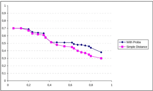
The mechanical parts in the collection contain holes so they can be fixed to other mechanical parts. Sometimes the positions and the dimensions of the holes can differentiate between two models from the same class. Zernike moments give global information about the edge image of the 2D view. Table 2 shows performance in terms of the FT, ST, and NN. Figure 11 shows the recall precision plot, we can notice again the contribution of the probabilistic approach to the improvement of the results. The results show that the Zernike Moments give the best results on our models collection.
Figure 12 and 13 show an example of querying using Zernike moments with the probabilistic approach.. 0 0 , 1 0 , 2 0 , 3 0 , 4 0 , 5 0 , 6 0 , 7 0 , 8 0 , 9 1 0 0 , 2 0 , 4 0 , 6 0 , 8 1 W it h P r o b a S im p le D is t a n c e
Figure 11. Zernike moments overall recall precision. Courbe de rappel précision des moments de Zernike.
Performance Methods
FT ST NN
With Proba 55.77 82.33 72.88 Simple Distance 51,68 70.13 65.27
Table II. Zernike moments retrieval performances. Performances de l’indexation avec les moments de Zernike.
Figure 12. Request input is a random view of a model. La requête est une vue aléatoire d'un modèle.
Figure 13. Top 4 retrieved models from the collection with Zernike moments. Les 4 premiers résultats retournés avec les moments de Zernike.
V.3. Curvature Scale Space (CSS)
As mentioned before, the collection used in the tests is provided by the car manufacturer Renault and is composed of mechanical parts. Most of the mechanical parts and due to industrial reasons do not have a curved shape. The main information in the CSS is the salient curves, which in the occurrence are rare in the shapes of the models. This particularity of our current collection explains the problem with the curvature scale space. In the cases where the model shape is curved, the recognition rate is very high, but in most 3D model from our collection, the shape is not much curved. Table 3 shows performance in terms of the FT, ST, and NN. Figure 14 shows the recall precision plot, we can notice again the contribution of the probabilistic approach to the improvement of the results. The results show that the Curvature Scale Space do not give accurate results on our models collection. 0 0,1 0,2 0,3 0,4 0,5 0,6 0,7 0,8 0,9 1 0 0,2 0,4 0,6 0,8 1 With Proba Simple Distance
Figure 14. Curvature Scale Space overall recall precision. Courbe de rappel précision des Curvature Scale Space (CSS).
Performance Methods
FT ST NN
With Proba 25.13 39.13 51.37 Simple Distance 24.98 35.1 49.278
Table III. Curvature Scale Space retrieval performances. Performances de l’indexation avec les Curvature Scale Space (CSS).
Figure 15 and 16 show an example of querying using Curvature Scale Space with the probabilistic approach. The request image is a model that gives good results with CSS due to the curves it contains.
Figure 15. Request input is a random view of a model. La requête est une vue aléatoire d'un modèle.
Figure 16. Top 4 retrieved models from the collection with Curvature Scale Space. Les 4 premiers résultats retournés avec les Curvature Scale Space.
V.4. Real photos tests
One of the main goals of the SEMANTIC-3D project is to provide car technicians a tool to retrieve mechanical parts references. The solution proposed is to retrieve objects that correspond the most to a photo of the mechanical part.
As mentioned before, our framework can accept many descriptors, but not all of them are suitable for the retrieval of 3D CAD models from a photo.
Curvatures Histogram?
The main problem with the curvature histogram is its dependency on the light position. A small change in the lightening make changes in the curvature, that leads to a difference in the curvature histogram. Not suitable!
Curvature Scale Space?
Most of the mechanical parts and due to industrial reasons do not have a curved shape. The main information in the CSS is the salient curves, which in the occurrence are rare in the shapes of the models. This particularity of our current collection explains the problem with the Curvature Scale Space. Not suitable!
Zernike Moments?
The mechanical parts in the collection contain holes so they can be fixed to other mechanical parts. Sometimes the positions and the dimensions of the holes can differentiate between two models from the same class. Zernike moments give global information about the edge image of the 2D view. These properties of the Zernike moments make it the most suitable for 3D model retrieval from photos.
During the rest of the paper and for our tests we used the Zernike moments descriptors for the reasons mentioned in the previous sections.
To use our algorithms presented in the previous sections on real photos, a pre-processing stage is needed. As the photos will be compared to views of the 3D models, we make a simple segmentation using a threshold. A more sophisticated segmentation can be used, but it is behind the scope of this paper. Then Zernike moments are calculated on the edge image made by the Canny filter.
Figure 17 shows a wheel from a Renault car. Figure 18 shows the 3D models results to this request using our retrieval system with their respective ranks.
Figure 17. A request photo representing a car wheel. Une photo requête représentant un volant de voiture.
Figure 18. Results for the car wheel photo (figure 17). Résultats pour le volant de voiture (figure 17).
Figures 19 shows a low resolution photo (200x200 pixels) of wheel from a Renault car. The figure 20 show the 3D models results to this request using our retrieval system with their respective rank.
Figure 19. A low resolution request photo representing a car wheel. Une photo basse résolution représentant un volant de voiture.
Figure 20. Results for the car wheel photo (figure 19). Résultats pour le volant de voiture (figure 19).
VI. Conclusion and future work
We have presented a new framework to extract characteristic views from a 3D model. The framework is independent from the descriptors used to describe the views. We have also proposed a bayesian probabilistic method for 3D models retrieval from a single random view.
Our algorithm for characteristic views extraction let us characterise a 3D model by a small number of views.
Our method is robust in terms of shape representations it accepts. The method can be used against topologically ill defined mesh-based models, e.g., polygon soup models. This is because the method is appearance based: practically any 3D model can be stored in the collection.
The evaluation experiments showed that our framework gives very satisfactory results with different descriptors. In the retrieval experiments, it performs significantly better when we use the probabilistic approach for retrieval.
Our preliminary results on real photos are satisfactory, but more sophisticated methods for segmentation and extraction from background must be used.
In the future, we plan to focus on real images, and also to adapt our framework to 3D/3D retrieval and test it on larger collection.
VII. Acknowledgements
This work has been supported by the French Research Ministry and the RNRT (Réseau National de Recherche en Télécommunications) within the framework of the SEMANTIC-3D National Project (http://www.semantic-3d.net).
VIII. Bibliography
[1] Vandeborre (J.P.), Couillet (V.) and Daoudi (M.), "A Practical Approach for 3D Model Indexing by combining Local and Global Invariants", 3D Data Processing Visualization and Transmission (3DPVT), pp. 644-647, Padova, Italy, june 2002.
[2] Sundar (H.), Silver (D.), Gagvani (N.) and Dickinson (S.), "Skeleton Based Shape Matching and Retrieval", IEEE proceedings of the Shape Modeling International 2003 (SMI'03).
[3] Abbasi (S.), and Mokhtarian (F.), "Affine-Similar Shape Retrieval: Application to Multi-View 3-D Object Recognition", IEEE Transactions on Image Processing, Volume 10, Number 1, pp. 131-139, 2001.
[4] Dorai (C.) and Jain (A.K.), "Shape Spectrum Based View Grouping and Matching of 3D Free-Form Objects", IEEE Transactions on Pattern Analysis and Machine Intelligence, Volume 19, Number 10, pp.1139-1146, 1997. [5] Mahmoudi (S.) et Daoudi (M.), "Une nouvelle méthode d'indexation 3D",
13ème Congrès Francophone de Reconnaissance des Formes et Intelligence Articifielle (RFIA2002), volume 1, pp. 19-27, Angers, France, 8-9 janvier 2002.
[6] Chen (J-L.) and Stockman (G.), "3D Free-Form Object Recognition Using Indexing by Contour Feature", Computer Vision and Image Understanding,
Volume 71, Number 3, pp.334-355, 1998.
[7] Yi (J.H.) and Chelberg (D.M.), "Model-Based 3D Object Recognition Using Bayesian Indexing", in Computer Vision and Image Understanding, Volume 69, Number 1, January, pp.87-105,1998.
[8] Chen (D.Y.), Tian (X.P), Shen (Y.T.) and Ouhyoung (M.), "On Visual Similarity Based 3D Model Retrieval", Eurographics 2003, Volume 22, Number 3.
[9] Chen (D.Y.) and Ouhyoung (M.), "A 3D Model Alignment and Retrieval System", Proceedings of International Computer Symposium, Workshop on Multimedia Technologies, Vol. 2, pp. 1436-1443, Hualien, Taiwan, Dec. 2002. [10] Ohbuchi (R.), Nakazawa (M.), Takei (T.), “Retrieving 3D Shapes Based On Their Appearance”, Proc. 5th ACM SIGMM Workshop on Multimedia Information Retrieval (MIR 2003), pp. 39-46, Berkeley, Californica, USA, November 2003.
[11] Costa (M.S.) and Shapiro (L.G.), "3D Object Recognition and Pose with relational indexing", Computer Vision and Image Understanding, Volume 79, pp. 364-407, 2000.
[12] Tangelder (J.W.H.), Veltkamp (R.C.), "A survey of content based 3D shape retrieval methods"; Shape Modeling International, 2004, Proceedings,7-9 june 2004 Pages:145-156
[13] Koenderink (J.J.) and Van Doorn (A.J.), "Surface shape and curvature scales",
Image and Vision Computing, Volume 10, Number 8, pp. 557-565, 1992. [14] Nastar (C.), "The image Shape Spectrum for Image Retrieval", INRIA
Technical Report number 3206, 1997.
[15] Zaharia (T.), Prêteux (F.), "Indexation de maillages 3D par descripteurs de forme", 13ème Congrès Francophone de Reconnaissance des Formes et Intelligence Artificielle (RFIA2002), volume 1, pp. 48-57, Angers, France, 8-9 janvier 2002.
[16] Kim (W.Y.), Kim (Y.S.), “A region-based shape descriptor using Zernike moments”, Signal Processing: Image Communication, Volume16, (2000), pp 95-100.
[17] Khotanzad (A.) and Hong (Y. H.), “Invariant image recognition by Zernike moments”, IEEE Transactions on Pattern Analysis and Machine Intelligence , Volume 12, No.5, May 1990.
[18] Daoudi (M.), Matusiak (S.), "Visual Image Retrieval by Multiscale Description of User Sketches", Journal of Visual Languages and computing, special issue on image database visual querying and retrieval, Volume 11,pp 287-301, 2000.
[19] Mokhtarian (F.) and Mackworth (A.K.), "Scale-Based Description and Recognition of Planar Curves and Two-Dimensional Shapes, IEEE Transactions on Pattern Analysis and Machine Intelligence, vol. 8, no. 1, pp. 34-43, 1986.
[20] Eberly (D. H.), "Geometric Methods for analysis of Ridges in N-Dimensional Images", PhD Thesis, University of North Carolina at Chapel Hill, 1994.