Computer-aided definition of sizing procedures and optimization problems of mechatronic systems

HAL Id: hal-01861795

https://hal.archives-ouvertes.fr/hal-01861795

HAL is a multi-disciplinary open access archive for the deposit and dissemination of sci-entific research documents, whether they are pub-lished or not. The documents may come from teaching and research institutions in France or abroad, or from public or private research centers.

L’archive ouverte pluridisciplinaire HAL, est destinée au dépôt et à la diffusion de documents scientifiques de niveau recherche, publiés ou non, émanant des établissements d’enseignement et de recherche français ou étrangers, des laboratoires publics ou privés.

Computer-aided definition of sizing procedures and

optimization problems of mechatronic systems

Aurelien Reysset, Marc Budinger, Jean-Charles Maré

To cite this version:

Aurelien Reysset, Marc Budinger, Jean-Charles Maré. Computer-aided definition of sizing procedures and optimization problems of mechatronic systems. Concurrent Engineering: Research and Applica-tions, SAGE PublicaApplica-tions, 2015, 23 (4), pp.320 - 332. �10.1177/1063293X15586063�. �hal-01861795�

Computer aided definition of sizing procedures and optimization problems of mechatronic systems Aurélien Reysset1_{, Marc Budinger}1 _{and Jean-Charles Maré}1

1 _{Toulouse University, INSA/UPS, Clément Ader Institute, Toulouse, France}

Abstract

This paper is dedicated to the generation of sizing procedures used during the preliminary optimal design of physical parts of mechatronic systems. The knowledge necessary to such design is composed of 2 layers: mechatronic system layer and component layer. Such knowledge can be represented by algebraic equations directly or by the use of meta-modelling techniques. Constraint networks and graphs theory are used here to represent and order the constraints and the links between those algebraic models in order to obtain a well-posed optimization problem. The selected or developed algorithms are finally illustrated with typical prob-lems of component selection.

Key words

Mechatronics, system design, optimized sizing procedure, graph theory, matching-ordering algorithm.

From models to optimal preliminary design of mechatronics systems

Preliminary design of mechatronic systems

A mechatronic system [1] expands the capabilities of conventional mechanical systems through the inte-gration of different technological areas around a power transmission part and an information processing part. The references [2] [3] highlight the fact that the design of such multi-domain systems requires different modelling layers as represented in Figure 1:

1. A mechatronic system layer, to take into account the functional and physical coupling between com-ponents. This level of modelling is usually done using 0D-1D models also called lumped parameter models represented by algebraic equations, ordinary differential equations (ODE) or differential alge-braic equations (DAE) [4]. During preliminary design, these models represent sizing scenarios. Meta-modelling techniques often enable to represent those models by algebraic equations for a quicker op-timization [5].

2. A specific domain/component layer, to describe the performance limits and parameters necessary in the previous layer, based on a geometric representation. The specific domain phenomena are generally represented through partial differential equations (PDE). This level of modelling can be achieved, for simplified geometries by using analytical models or, for complex 2D and 3D geometries, by using numerical approximations like the finite element method (FEM) for instance. During preliminary de-sign and optimization, this layer can be represented by analytical models, meta-models [6] or scaling laws [7].

Sizing procedure vs. optimization

Generally the engineering models enable to determine the opposite relationship to what is desired during sizing, i.e. calculate the performance of the system (which is required by the specification) from the char-acteristics of components (which sizing activities want to define). All representative models have to be manipulated in order to solve this inverse problem. There are essentially two types of solutions:

1. Selection or sizing procedures, judicious succession of calculations and tests which determine the main characteristics of components to select.

2. Optimization algorithms that minimize the difference between the desired and achieved performances by changing the main characteristics of components.

In this paper, the goal is to make joint use of these two approaches, sizing procedures and optimization, combined to mechatronic systems and components layers representation of knowledge. The next section will present a state-of-the-art overview of the different ways of representing a sizing procedure. We will focus on their generation by using simple graphical means or by using algorithms from graph theory. The different approaches and issues will finally be illustrated with simple but typical examples.

State of the art on Sizing procedure representations

The sizing procedure can be considered as a major part of the whole preliminary sizing process. When the problem is complex, the methods that represent all the interactions between components from various fields (mechanical, electrical, etc.), become valuable. This section focuses on representation methods.

Causal diagram

The causal diagram is a graphical tool representing the causal relationships between variables. It is in fact an oriented graph representing a calculation scheme. Examples of causal diagrams can be found in [8] or [9]. With a causal diagram, the couplings between the different entities may be difficult to visualize. An important problem is that of algebraic loops, which is named circular reference errors in spreadsheets, and is characterized by relations such as y=f(x) and x=g(y).

N² diagrams

The N² diagram formalism was introduced in the 70s by the system engineer Robert J. Lano [10]. N gives the number of entities considered. This diagram is a causal diagram where the graphical entities (blocks) and interactions (arrows) are dictated by an organization convention as shown in Figure 2a. The inputs of the blocks are represented by vertical arrows while the outputs must be horizontal arrows. This display provides a quick visual summary of the organization of the system studied. In particular, the couplings and algebraic loops between blocks are easily identifiable: for example, Figure 2 highlights coupling between block "2" and block "3".

DSM matrix

A Design Structure Matrix or Dependency Structure Matrix (DSM) is the adjacency matrix of a N² diagram (an example is given in Figure 2b). The DSM, as its name says is a matrix representing links or information exchanges which can be used at various levels: working group, system level [11], or component level fo-cussing on modularity analysis [12]. In this representation, a perfect straightforward sequence is represented by a lower triangular matrix, while the upper non-empty box represents a feedback design loop.

Graphs

Finally, a sizing procedure is quite similar to a constraint network [13] [14] [15], since sizing parameters represent variables, equalities and inequalities are viewed as constraints. Therefore, all the tools applied to the representation of constraints network and therefore graph theory can be applied. That is why various

algorithms applied to graph theory can be integrated to a global calculation ordering method. In the follow-ing sub-parts, different graphical representations will be used. Some of them represent how equations will match parameters; in this case both equations (square node) and non-determined parameters (circular node) are represented in a non-oriented graph. Let’s take the non-oriented, declarative equations:

 

 

A matching is generally represented in what is called a bi-partite graph, Figure 3a-b, with on one side all the equations nodes and on the other side all the non-determined parameters nodes. Once equations are oriented, i.e. one parameter is matched to the equation or calculated by the equation, the matching param-eter/equation can be represented by a double-column, Figure 3b, or the information flow can be represented by oriented arrows, Figure 3c. The set of equations can also be represented by a dependency matrix (Figure 3).

Sizing procedure definition

Objectives

This section deals with the representation of a set of design calculations and the scheduling of information flows into a sizing procedure. In order to have a well-posed sizing procedure, easy to use in any computing environment, it must be explicit without internal numerical solver. For a complex problem gathering nu-merous equations and constraints, it might be not obvious to find a proper explicit sequence (no singularity and no loop), which is why the problem must be adapted.

Next sections will present: the typical inputs and outputs of such procedure which will be used in an opti-mization problem, the proposed methodology and process, how to set up manually a sizing procedure using graphical tools, a computer implementation using algorithms from graph theory, and finally how to identify the main typical problems that can occur with illustrations on elementary examples.

Inputs and outputs of an optimization problem

Minimize the objective function: f(x)

Subject to equality/inequality constraints: h(x)=0, g(x)<0 Acting on the parameters vector in the range: xlow<x<xup

Where:

1. The goal is the objective function f;

2. Design alternatives are expressed by a set of values assigned to the design variables x within a design domain;

3. Constraints (h & g) limit the number of alternatives to those satisfying physical principles and design specifications.

The functions (f, g, h) can be explicit or implicit, algebraic or achieved by subroutines that solve systems of differential equations iteratively. The goal here is to define those functions within a sizing procedure. This sizing procedure should be preferably explicit and quick to evaluate.

Ordering methodology and process

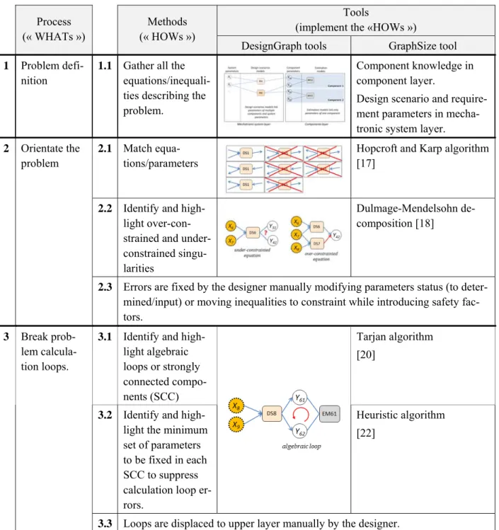
The equations ordering methodology is organized into 3 main steps summed-up in Table 1.

This global method helps to reveal additional design parameters and to structure the sizing procedure which can be used by an optimization algorithm.

This process of block lower triangulation may be applied to any type of knowledge represented by models. However, in the case of a mechatronic system, it is possible to distinguish two levels of knowledge:

1. A component layer that represents the specific domains knowledge for each component. This knowledge is represented by parameters (definition, integration, simulation, evaluation) and equations (estimation models) linking the parameters of only one component. Each set of equations and param-eters is component-independent and can thus be stored and reused in the form of a library.

specifications declined on all sizing scenarios. These models can link characteristics of multiple com-ponents from component layer freely.

“DesignGraph”: sizing procedure synthesis thanks to graphical manipulations

For design problems characterized by a reduced set of equations, a skilled designer will be able to order quickly and intuitively design constraints of his area of knowledge. However, it is also possible to graph-ically represent and order these equations. This graphical representation, here called "Design Graph", can be used as a teaching tool with students or as an analysis tool for an engineer in the case of new design scenarios or new technology.

The problem definition, Task 1 of Table 1, is achieved with a bipartite graph for each design layer as rep-resented in Figure 4a where:

1. The parameters are set at mechatronic system layer from requirements specifications (performances, constraints) and at components layer by listing the components of the architecture and their main char-acteristics.

2. The equations are then introduced to link the different parameters: at the mechatronic system layer level with equations representing design scenarios, at the components layer level with estimation mod-els.

At this point the relationships between the parameters and equations are represented as non-oriented edges. The orientation of the equations is the next step and corresponds to Task 2 from Table 1. The parameters with value imposed by the specifications are selected as inputs for the sizing procedure and can be removed from the matching process. Some parameters in the specification may take the form of outputs if the word-ing of the requirement defines them as an objective to minimize or maximize or as a maximum or minimum limit constraint to respect. Figure 4b summarizes the graphical notation that can be chosen to represent these parameters in a form approaching an influence diagram [16] in order to prepare the implementation of the optimization problem.

per calculation node (Figure 4c). If the same equation remains undetermined for several parameters (Figure 4d), some design assumptions have to be done by stating that some parameters are known. These new design parameters can be included in the optimization problem and their optimal value can be determined via the optimization algorithm. A preferred choice for these new design parameters is that of parameters participating in a large number of equations (such as gear reduction ratio) and values defined into a known range [min; max]. These assumptions allow to balance the number of equations available and the number of parameters to be determined by the calculation procedure. The first example of the last section illustrates this case of under-constrained problem.

If several equations of design scenarios have the same output, Figure 4d, the problem may be over-con-strained. Two solutions can be applied: by adding a safety factor and managing one of the equations as a constraint in the optimization problem or by giving the assignment to the most restrictive equation when direct comparison is possible. The second example of the last section illustrates this case of over-con-strained problem.

The treatment of possible algebraic loop is the last step and corresponds to Task 3 in Table 1. An algebraic loop can be typically found in the selection of a component involving the use of characteristics of this same component. This case is represented graphically by a loop involving a design scenario equation and an estimation model equation as shown in Figure 4d. Adding once again a new design parameter, such as an oversizing coefficient, and a constraint to be checked by the optimization algorithm makes the sizing pro-cedure explicit. The last example of the last section illustrates this case.

At the end of this graphical treatment, the final sequence of equations can be represented as an upper triangular N² diagram or as a lower triangular matrix (Figure 2) in order to check that the sequence of equations is explicit.

“GraphSize”: sizing procedure synthesis through algorithmic manipulations

In the case of the design of a multi-domain product characterized by a large set of equations, it may be difficult for an engineer to write and order manually the equations properly in order to establish an explicit

and straightforward design procedure. A computer tool, that can help him do so, then becomes valuable. Here, an in-house Matlab implementation of such software, that we have called "GraphSize", is presented. For the problem definition, Task 1 in Table 1, "GraphSize" represents the equations and parameters in both components and mechatronic system layers, defined in the previous two paragraphs. This decomposition facilitates the reuse of models through component libraries (Component layer) or sizing scenario libraries (Mechatronic system layer). The relations, called “rules”, may take the form of equalities or inequalities. The tool automatically lists the parameters from the equations. These rules can be declared in an equation section, and will then be analysed to be ordered, or in a constraint section, and will then be used as con-straints only by the optimization algorithm remaining out of the ordering process.

The problem is thus defined by a given number of non-oriented equalities/inequalities. Most of the time, optimal values are obtained for a solution around the constraint. For example, for a motor where the design driver is the coil maximum temperature Tmax, the designer may check that Tcoil≤Tmax, leading to an

over-sized solution. But if in addition to that inequality, the motor mass has to be minimized, the final result will tend to an equality Tcoil=Tmax. Therefore, at first, inequalities in the equations section will be considered as

equalities and only if the problem is over-constrained, some adaptation will be made adding over-sizing parameters and moving inequalities to the constraints section in order to decrease over-constraint order. So, having a problem of ‘n’ equations functions of ‘m’ unknown parameters, it will be first interesting to assign one output parameter to each equation in order to orient the problem. The orientation of the equations corresponds to Task 2 in Table 1.

This means that the equations will be transformed as follows:









f1 1, 2,..., 0 2  1' 1, 3,..., (3) To ensure that the assignment number is as high as possible, an augmenting path method will be applied. This method is based on the matching Hopcroft & Karp algorithm [17]. Before applying the H&K algo-rithm, a heuristic method is applied to match equations (rows) and parameters (columns). It consists in matching each equation to the first free column encountered that is linked to the row, repeating the principle

from first to last row. Then, if the matching is lower than the maximum possible assignment (lowest matrix dimension), H&K is applied to an assigned matrix. The algorithm presented in [17], consists in two steps: a breadth first search (BFS) and a depth first search (DFS), repeated till the assignment does not increase. It must be applied to a graph that is not disjoint (i.e. all the nodes are reachable by performing a DFS or BFS with a single starting node):

1. Generate the graph by applying a BFS starting from all currently free row nodes (equations) and stop-ping when a first free column node (parameter) is encountered. During this step, while descending the graph tree, a parameter node is linked to its matching equation node, while an equation is linked to the remaining parameters. During the BFS, dependency matrix crosses are replaced by level orders so as to identify the path orientation and simplify the following step.

2. Starting from a free column node, a DFS is applied crossing decreasing indices of the dependency matrix. Then, when an augmenting path is encountered, matching along the path is modified and the algorithm returns to step 1.

The next step will identify parts of the problem presenting under-constrained or over-constrained singular-ities [18]. Of course, if n≠m, the problem is singular, but we will see that n=m does not necessarily mean the problem is not singular. This step may help the designer to fix parameters as inputs and move inequal-ities from equations to constraints (handled by the optimization upper-layer).

When the equation orientation has been done, the dependency matrix, as shown in Figure 3, can be drafted, feedback loops and strongly connected components (SCC) will be extracted thanks to a Tarjan algorithm [19] [20]. And here comes the last step of the method (Task 3 of Table 1). For each SCC, a heuristic algorithm finds the minimal number of internal parameters to fix in order to determine all the other param-eters encountered in the SCC [21] [22]. Normally, these particular paramparam-eters are used as initial inputs to the numerical iteration loops, and then all other parameters are obtained and will lead to a new estimation of the inputs values, looping until the error between fixed and estimated value falls below an acceptable threshold. In our case, the SCC input parameters will be extracted at input level and defined within a range, then the value calculated within SCC will be compared to the input through an additional constraint handled

by the optimization layer. These problem solving choices were driven by the wish to use an independent solver generating a standard code which can be imported into as many calculation/optimization environ-ments as possible.

Typical problems

Global concepts were presented in previous parts. The idea is now to present a few examples to highlight the value of such methods especially regarding singularity and loop issues. The examples discussed here are deliberately simple to facilitate the demonstration but deal with each typical issue encountered in the implementation of sizing procedure. They are based on servo-hydrostatic (SHA) and electromechanical actuators (EMA) sizing (Figure 5).

Under-constrained singularity: hydraulic jack

The aim is to implement the selection procedure of a hydraulic servo-actuator (jack and servo-valve) to ensure a rated load F0 and a rated speed V0 for a useful stroke dx. The anchorage structure has a stiffness K

and does not tolerate effort higher than Fmax. The maximum flow rate Qmax (no-load flow) required by the

actuator should be minimized to reduce the mass of the hydraulic supply system.

The physical equations for such a system are summed up here and can be represented by using a DesignGraph, as shown in Figure 6.

net P S F_max  . ₍₄₎ 0 .F K dx C  ₍₅₎ 0 0 S.P F  (6) S Q V₀ ₀/ (7)





Equations (5) to (7) refer to jack component and link the total stroke C, piston area S and rated flow Q0 to

respectively nominal component flow and pressure drop features.

From the listed parameters, some will be determined as input by the customer’s specification document, F0,

V0, dx, Pnet and K; while others are objective, Qmax which must be minimized, or constraint, Fmax≤Fstructure

limited by maximum allowable load of the structure (optimization upper-layer). With these choices the problem is reduced to 6 equations - 8 parameters and is even undetermined.

The design graph allows to highlight the sub-constraints: calculation nodes 6 to 8 (Figure 6a-b) indeed require to assume that 2 parameters are known to allow the sequencing of computations. As dPnom may be

given as a test definition by the valve technology, it may be taken as input and P0 is easy to limit to a range

equal to [0; Pnet], so it will be taken as second input (variable). A new sequence of equations, given Figure

6c-d, fixes and solves under-constrained singularity.

An optimization problem with P0 as design parameter, Qmax as objective and Fmax as constraint is thus

ob-tained. The optimization enables to find a classical hydraulic design rule: the pressure P0 must be equal to

2/3 of Pnet in order to minimize Qmax.

Over-constrained singularity: rollers-screw

Here will be presented an over-constrained problem which is quite simple but which will allow to present the way to solve this kind of singularity. The objective is to select a roller screw subjected to two constraints: a static load Fmax and a dynamic load representing rolling fatigue FRMC.

The problem can be divided this time by using the two above-mentioned layers, beginning with the com-ponent layer and roller-screw scaling laws explained in [7].













Where F0 and Fd are respectively rollers-screw static and dynamic definition load, Ln the nut length and ms

the screw mass per unit length. A ‘ref’ index refers to reference component features. The screw total mass

s s

s m L

M  . (13)

Where the screw total length Ls comes from the mechatronic system layer equation:

b n

s C L L

L    ₍₁₄₎

It’s in fact the sum of the useful actuator stroke C, the nut length and the thrust bearing length Lb.

The last two equations are constraints expressed at mechatronic system layer and insuring proper use of the rollers-screw: max 0 F F  ₍₁₅₎ RMC d F F  (16)

As reference component data (ms,ref, F0,ref,…) and specifications (Fmax and FRMC) are available, and as thrust

bearing will be considered to be sized first, then the problem is in fact 7 equations with 6 undetermined parameters (Figure 7a).

The obtained matrix (Figure 7b) clearly highlights that one of the last 3 equations must be removed to obtain non-singular problem. To do so, one of the inequalities must be displaced to constraints, equation (16) for example.

Yet, without modifying the other equation (considered as: F0=Fmax), if fatigue is the sizing criteria, the

constraint will never be met. That is why a degree of freedom ‘kc’ must be introduced to the equation:

max

0 k .F

F  _c (17)

With kc a variable input here within the range [1; +∞]. Then the final result is the one presented in the

Figure 7c, where kc will represent an over-sizing coefficient to validate dynamic sizing.

Algebraic loop: brushless electric motor

The purpose of the last example is to highlight algebraic loop within a sizing procedure. To do so, a brush-less electric motor will be sized considering only the maximum transient torque it has to deliver T0. This

torque is calculated at mechatronic system layer as the sum of transient application load demand Tload and

w load Jd T

T₀  . (18)

Then, applying scaling laws of [7], the following equations of inertia and mass M are obtained using refer-ence properties:









As reference components such as torque and acceleration demands are determined, the problem is com-posed of 3 equations and 3 unknowns.

In Figure 8a-b, an algebraic loop appears since T0 and J computation are linked. To break the loop, an

oversizing coefficient km can be introduced to adapt equation (18) and reuse the original one as a constraint:

load mT k T₀ . ₍₂₁₎ w load Jd T T₀  . ₍₂₂₎

Another way to solve it, this time automatically with a heuristic program, is by fixing as input T0,f within

the range [Tload; 10.Tload]. Then, the algebraic loop does not exist anymore. Equation (18) is used as an

output estimator:

w load

e T Jd

T_0,   . ₍₂₃₎

The acceptance error criterion is described as a constraint: 



 _{f e}

e T T

T_{0, 0,} / _{0, (24)}

This new sizing procedure has no algebraic loop thanks to the introduction of a new design parameter and a new constraint for the optimization problem.

Conclusion

This paper has shown that preliminary design of mechatronic systems can be modeled by equations repre-sented into 2 layers, the mechatronics and the components layer, which enable storage of knowledge as libraries of non-oriented equations. Whenever a dynamic simulation representing the behavior of a key design indicator is needed, some effort can be done to replace it by an explicit meta-model formulation.

Anticipated simulation and modelling have two advantages: gathering knowledge and quickening the whole optimization. The optimization problem corresponding to the preliminary design is function of the sizing procedure definition which results of the ordering of the calculation steps. This paper has proposed graph-ical representation, based on graphs representation and algorithms that can be applied to highlight the dif-ferent problems the designer has to face (singularity, calculation loop) during the generation of this sizing procedure.

Finally the problem is formulated in an explicit way which can be implemented in as many solvers/optimi-zation tools as possible.

Funding

The research was carried out as part of a European Union funded 7th Framework Program project – ACTUATION 2015 (Modular Electro Mechanical Actuators for ACARE 2020 Aircraft and Helicopters) (grant number 284916).

Corresponding author:

Marc Budinger, INSA Toulouse, Clément Ader Institute, Toulouse, 31077, France. Email: marc.budinger@insa-toulouse.fr

References

[1] D. Auslander, «What is mechatronics?,» Mechatronics, IEEE/ASME Transactions on, vol. 1, n° %11, pp. 5-9, march 1996.

[2] H. Van der Auweraer, J. Anthonis, S. De Bruyne et J. Leurdian, «Virtual engineering at work: the challenges for designing mechatronic products,» Engineering with Computers, vol. 29, pp. pp. 389-408, 2013.

[3] P. Hehenberger, F. Poltschak, K. Zeman et W. Amrhein, «Hierarchical design models in the mechatronic product development process of synchronous machines,» Mechatronics, vol. 20, pp. pp. 864-875, 2010. [4] F. Cellier et J. Greifeneder, Continuous System Modeling, Springer, Éd., 1991.

[5] M. Budinger, A. Reysset, T. El Halabi, C. Vasiliu et J.-C. Maré, «Optimal preliminary design of electromechanical actuators,» Proceedings of the Institution of Mechanical Engineers, Part G: Journal of

Aerospace Engineering, vol. 228, n° %19, p. pp 159, 2014.

[6] M. Budinger, J.-C. Passieux, C. Gogu et A. Fraj, «Scaling-law-based metamodels for the sizing of mechatronic systems,» Mechatronics, n° %1doi: 10.1016/j.mechatronics.2013.11.012., 2014.

[7] M. Budinger, J. Liscouet, J. Mare et others, «Estimation models for the preliminary design of electromechanical actuators,» Proceedings of the Institution of Mechanical Engineers, Part G: Journal of

Aerospace Engineering, vol. 226, n° %13, pp. 243-259, 2012.

[8] Salome, 2014. [En ligne]. Available: www.salome-platform.org/about/yacs.

[9] S. Liscouet-Hanke et K. Huynh, «A Methodology for Systems Integration in Aircraft Conceptual Design – Estimation of Required Space,» chez SAE Technical Paper, 2013.

[10] NASA, Techniques of Functional Analysis, NASA Systems Engineering Handbook, 1995.

[11] B. Shekar, R. Venkataram et B. Satish, «Managing complexity in aircraft design using design structure matrix,» Concurrent Engineering vol.19, pp. 283-294, December 2011.

[12] C. Qiang, Z. Guojung et S. Xinyu, «A product module identification approach based on axiomatic design and design structure matrix,» Concurrent Engineering vol. 20, pp. 185-194, 2012.

[13] G. Friedman et C. Leondes, «Constraint theory, part I: fundaments,» IEEE transactions on systems science

and cybernetics, vol. 5, n° %11, pp. 48 - 56, Janvier 1969.

[14] D. Serrano, «Contraint management in conceptual design,» Cambridge, 1987.

[15] E. Gelle et B. Faltings, «Solving mixed and conditional constraint satisfication problems,» Kluwer academic

publishers, pp. 107-141, 2003.

[16] R. J. Malak, L. Tucker et C. Paredis, «Compositional modelling of fluid power systems using predictive tradeoff models,» International of fluid power, vol. Vol. 10, n° %12, pp. 45-56, 2009.

[17] I. Duff et T. Wiberg, «Remarks on implementations of O(n1/2 τ) assignment algorithms,» ACM transactions

on mathematical software, vol. Vol. 14, n° %13, pp. 267-287, 1988.

[18] A. Pothen et C. Fan, «Computing the block triangular form of a sparse matrix,» ACM transactions on

mathematical software, vol. vol. 16, n° %14, pp. 303-324, 1990.

Grenoble, 2003.

[20] J. Helary, Algorithmique des graphes, Rennes university publication, 2004.

[21] M. J. Buckley, K. W. Fertig et D. E. Smith, «Design Sheet: An Environment for Facilitating Flexible Trade Studies During Conceptual Design,» chez Aerospace Design Conference, Irvine, California, 1992.

[22] S. Reddy, K. Fertig et D. Smith, «Constraint management methodology for conceptual design tradeoff studies,» chez Proceedings of the ASME design engineering technical confetence, 1996.

[23] blablabla, «Computing the block triangular form of a sparse matrix,» ACM transactions on mathematical

software, vol. 16, no. 4, pp. 303-324, 1990..

Author biographies

Aurelien Reysset is a PhD candidate at Clement Ader Institute and INSA Toulouse. He has an MSc degree in Mechanical and Systems engineering from INSA Toulouse. His PhD stud-ies are funded by the Actuation 2015 European project and focus on design methodologstud-ies and tools, KBE and optimization for aerospace actuation systems.

Marc Budinger received the Aggregation degree in Applied Physics in 1998 and the PhD degree in Electrical Engineering from Polytechnic National Institute of Toulouse in 2003. He is now associate professor with the Mechanical Engineering Department of INSA Toulouse and his current research topic, at Clement Ader Institute, deals with modeling and simulation for the preliminary design of electromechanical actuators.

Jean-Charles Mare got his French engineering degree in mechanics in 1982 at INSA Tou-louse. Pr. Mare has acquired more than 25 year experience in system level simulation of aerospace actuators and actuation systems. He has been involved in industrial and research projects for commercial aircrafts, helicopters, weapons and test benches. His field of expertise for the system level modelling and virtual prototyping concerns essentially the hydraulic and mechanical power transmission and control.

Table 1. Synthesis of the proposed methodology Process (« WHATs ») Methods (« HOWs ») Tools

(implement the «HOWs »)

DesignGraph tools GraphSize tool 1 Problem

defi-nition

1.1 Gather all the equations/inequali-ties describing the problem.

Component knowledge in component layer.

Design scenario and require-ment parameters in mecha-tronic system layer. 2 Orientate the

problem

2.1 Match equa-tions/parameters

Hopcroft and Karp algorithm [17]

2.2 Identify and high-light over-con-strained and under-constrained singu-larities

Dulmage-Mendelsohn de-composition [18]

2.3 Errors are fixed by the designer manually modifying parameters status (to deter-mined/input) or moving inequalities to constraint while introducing safety fac-tors.

3 Break prob-lem calcula-tion loops.

3.1 Identify and high-light algebraic loops or strongly connected compo-nents (SCC) Tarjan algorithm [20]

3.2 Identify and high-light the minimum set of parameters to be fixed in each SCC to suppress calculation loop er-rors.

Heuristic algorithm [22]

a) Problem definition: components and Mechatronic system layers

b) Highlight of optimization inputs (design parameters) and outputs (objectives or constraint)

c) Equation orientation: single output

d) Typical encountered problems

a) Servo-hydrostatic actuator

b) Electromechanical gear-drive actuator Figure 5. Typical problems case study

a) Servo-hydraulic actuator definition graph

b) Dependency matrix highlighting singularity c) Dependency matrix of the adapted problem

d) Final optimization problem and embedded calculation sequence

a) Roller-screw sizing definition graph

b) Dependency matrix highlighting singularity c) Dependency matrix of the adapted problem Figure 7. EMA roller-screw sizing problem adaptation (graph and matrices)

a) Motor sizing definition graph

b) Dependency matrix highlighting algebraic loop Figure 8. EMA brushless motor sizing problem adaptation (graph and matrix)