An automatic geometrical and statistical method to detect acoustic shadows in intraoperative ultrasound brain images

HAL Id: inria-00432724

https://hal.inria.fr/inria-00432724

HAL is a multi-disciplinary open access

archive for the deposit and dissemination of sci-entific research documents, whether they are pub-lished or not. The documents may come from

L’archive ouverte pluridisciplinaire HAL, est destinée au dépôt et à la diffusion de documents scientifiques de niveau recherche, publiés ou non, émanant des établissements d’enseignement et de

An automatic geometrical and statistical method to

detect acoustic shadows in intraoperative ultrasound

brain images

Pierre Hellier, Pierrick Coupé, Xavier Morandi, D. Louis Collins

To cite this version:

Pierre Hellier, Pierrick Coupé, Xavier Morandi, D. Louis Collins. An automatic geometrical and statistical method to detect acoustic shadows in intraoperative ultrasound brain images. Medical Image Analysis, Elsevier, 2010, 14 (2), pp.195-204. �10.1016/j.media.2009.10.007�. �inria-00432724�

An automatic geometrical and statistical

method to detect acoustic shadows in

intraoperative ultrasound brain images

Pierre Hellier

∗, Pierrick Coup´e

, Xavier Morandi

and D.Louis Collins

a_{INRIA, IRISA, Campus de Beaulieu, Rennes, France}

b_{INSERM, VisAGeS U746 Unit/Project, Campus de Beaulieu, Rennes, France} c_{University of Rennes 1 - CNRS, IRISA, Campus de Beaulieu, Rennes, France} d_{University Hospital of Rennes, Department of Neurosurgery, Rennes, France}

e_{Montreal Neurological Institute, McGill University, Montreal, Canada}

Abstract

In ultrasound images, acoustic shadows appear as regions of low signal intensity linked to boundaries with very high acoustic impedance differences. Acoustic shad-ows can be viewed either as informative features to detect lesions or calcifications, or as damageable artifacts for image processing tasks such as segmentation, regis-tration or 3D reconstruction. In both cases, the detection of these acoustic shadows is useful. This paper proposes a new method to detect these shadows that combines a geometrical approach to estimate the B-scans shape, followed by a statistical test based on a dedicated modeling of ultrasound image statistics. Results demonstrate that the combined geometrical-statistical technique is more robust and yields bet-ter results than the previous statistical technique. Integration of regularization over time further improves robustness. Application of the procedure results in 1) im-proved 3D reconstructions with fewer artifacts, and 2) reduced mean registration error of tracked intraoperative brain ultrasound images.

Key words: 3D ultrasound, acoustic shadows, reconstruction, registration

∗ Tel: +33/0 2 99 84 25 23 / Fax: +33/0 2 99 84 71 71 Email address: pierre.hellier@irisa.fr (Pierre Hellier). URL: http://www.irisa.fr/visages (Pierre Hellier).

1 Introduction

The image formation process of ultrasound images is bound to the propaga-tion and interacpropaga-tion of waves in tissues of various acoustic impedances [1]. More precisely, at the boundary of two materials, the wave energy is trans-mitted, reflected, dispersed and/or diffracted. If the wave energy is almost totally reflected, this will result in an acoustic shadow in the region of the image beyond the boundary. The motivation for detecting acoustic shadows is twofold. First, the presence of an acoustic shadow reflects the presence of an interface where the acoustic energy was almost completely lost. This is typ-ically an interface tissue/air or tissue/bone. Therefore, acoustic shadows are useful to detect calcifications, gallstones or bone structures, detect lesions [2], discriminate benign tumors [3], predict stability of Peyronie’s disease [4] or di-agnosis leiomyoma [5]. Secondly, acoustic shadows might limit the efficiency of image processing techniques like segmentation, registration [6, 7] or 3D recon-struction. The automatic processing of ultrasound in a quantitative analysis workflow requires to detect and account for acoustic shadows. This paper will focus on the impact of shadow estimation on image processing tasks and more precisely on 3D reconstruction and 3D registration of ultrasound intraopera-tive data.

2 Related work

Only a few papers have presented automatic methods to detect acoustic shad-ows. Methods can be broadly sorted in two groups: intensity-based meth-ods [2, 8] and geometric methmeth-ods [6, 7]. Intensity-based methmeth-ods rely on a direct analysis of the intensities to detect dark regions. Madabhusi et al. [8] describe a method that combines a feature space extraction, manual training and classification to discriminate lesions from posterior acoustic shadowing. Drukker et al. [2] use a threshold on a local skewness map to detect shadows. Geometric methods take into account the probe’s geometry and analyze intensity profiles along the lines that compose the B-scan. Leroy et al. [6] fit an heuristic exponential function to determine whether a shadow occurred, while Penney et al. [7] manually estimate the image mask to determine dark areas.

The method proposed in this paper is a hybrid method combining a geo-metrical approach with a modeling of ultrasound image statistics. Contrary to previous papers, the image mask, the probe geometry and the statistical detection threshold are estimated automatically. Rather than fitting heuris-tic function to detect shadows, a statisheuris-tical analysis is performed along each transducer line to detect potential shadows regions. These ruptures (or breaks)

along the intensity profiles are tested as potential shadow boundary with a statistical test based on a noise model estimation.

3 Method

3.1 Overview

The shadow detection procedure consists of two phases. Since the presence of acoustic shadows is bound to the geometry of the probe and to the propagation of the signal along the lines that compose the B-scan, it is necessary to estimate the probe’s shape in the first phase. The probe’s shape is related to the probe geometry (linear, curvilinear) and corresponds to the image mask in the B-scans (see figure 1-a). Then, in a second phase, a signal analysis is performed along the lines that compose the B-scan. An acoustic shadow is detected along a line when two criteria are met:

(1) A rupture along a line exists and

(2) The signal distribution after the rupture is statistically compliant with an estimated noise model.

3.2 B-scan geometry extraction

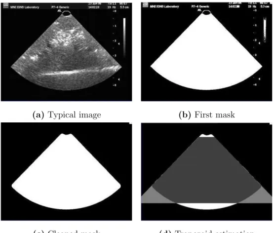
Given a sequence of 2D ultrasound images (see a typical image in figure 1-(a)), it is necessary to separate the image and the background. In many cases, the geometry (e.g., fan vs linear) will be known a priori, it will be possible to use a precomputed mask and this step of the procedure can be skipped. However, when this is not the case, estimating the mask amount to computing a 2D mask given the 2D + t sequence. To do so, maps of longitudinal mean and variance are computed, and multiplied pixelwise to compute a feature map. For a given point, the longitudinal mean (respectively variance) is defined as the mean (respectively variance) of a 2D pixel location over time. Background pixels are dark and have low (or zero) variance. Points in the image foreground have the highest values of the feature map (compared to the background). Then, points with the highest values of the feature map are retained (see figure 1-(b)). Some false detections exist, mainly due to textual data and complementary image information presented on the ultrasound machine display. Therefore, a morphological closing and opening are performed to clean the input mask (see figure 1-(c)). To estimate the probe geometry, a trapezoid model is fitted to the input mask. The trapezoid model is the simplest model capable of capturing the geometry of a linear or curvilinear probe. The 5 parameters of the model

are estimated by optimizing the total performance measure φ (see figure 1-(d)) that is defined as:

φ = T P + T N T P + T N + F P + F N

′

(1)

where T P is the number of true positives (point being in the mask and in the trapezoid), T N the number of true negatives (point being neither the mask nor in the trapezoid), F P the number of false positives (point not being in the mask but in the trapezoid) and F N the number of false negatives (point being in the mask but not in the trapezoid). With the symmetry hypothesis, the number of parameters is reduced to 4 and they are estimated within a simplex optimization. Thus the final shape will share as many points as possible with the mask, while maintaining the trapezoidal constraint.

For the model estimation, accuracy is needed for the extremal lines of the trapezoid. The extremal lines are the extreme right and extreme left lines that encompass the B-scans. Actually, these extremal lines are the most important features in the method, since they define the line profiles that will be triggered. Several experiments were conducted with three different acquisition systems (various video acquisition cards and echographic machines) and demonstrated that the method performs robustly in all tested cases. The mask in 1-(c) is used to determine which data will be analyzed for possible shadows, while the trapezoid in 1-(d) is used to determine the geometry of the US transducer lines (rays).

3.3 Line rupture detection

Once the probe’s geometry is estimated, it is possible to know whether the direction of scanning is top-down or bottom-up when a curvilinear probe is used. For a linear probe, the user must specify the direction of scanning (it is generally top-down except if the video grabber flipped the image). Afterwards, it is necessary to sample line profiles corresponding to the transducer lines. For each B-scan, an arbitrary number of lines can be drawn and for each line, k samples are computed by trilinear interpolation in the corresponding B-scan. As mentioned previously, the shadow is defined as a signal rupture along the line, followed by a low signal afterwards. Therefore, signal ruptures are detected first. To do so, the line signal is smoothed with a low-pass filter. Then, a local symmetric entropy criterion is computed. For each point p of the line signal S, a sliding window of size n is used to compute the rupture

(a) Typical image (b) First mask

(c) Cleaned mask (d) Trapezoid estimation

Fig. 1. Illustration of the automatic mask extraction. (a) shows a typical image of the acquired sequence. (b) shows the first mask obtained after selecting the highest values of the longitudinal statistics. (c) shows the mask after morphological opera-tors were applied to remove patient information. (d) shows the final trapezoid model estimation. criterion R: R = i=n X i=1 S(p − i) logS(p − i) S(p + i) + S(p + i) log S(p + i) S(p − i) !

The first term is the relative entropy of the ”past” (the signal before the rupture) knowing the ”future” (the signal after the rupture) which can also be viewed as the Kullback-Leibler divergence of the past distribution given a reference signal (the future). In order to symmetrize the criterion, the second term is added and expresses the relative entropy of the future knowing the past. The loci where R is maximal indicate a signal rupture. The rupture criterion R is quite general since it relies on the statistical dependency between the future and the past samples in a sliding window. Rupture positions are determined as zero-crossings of the gradient of R. Figure 2 illustrates the rupture detection on a synthetic example.

! "! #!! #"! $!! $"! %!! ! $! &! '! (! #!! #$! #&! ! "! #!! #"! $!! $"! %!! $! &! '! (! ! "! #!! #"! $!! $"! %!! ! "!! #!!! #"!! $!!! $"!!

(a)Input signal (b) Attenuation (c) Added noise

! "! #!! #"! $!! $"! %!! $!! &!! '!! (!! #!!! #$!! #&!! ! "! #!! #"! $!! $"! %!! ! #!!! $!!! %!!! &!!! ! "! #!! #"! $!! $"! %!! &$!! &#!! ! #!! $!!

(d)Filtered signal (e) Rupture detection (f )Rupture gradient Fig. 2. Illustration of the line processing on a synthetic signal. (a) : a synthetic ”hat” signal is used as an input. (b) : an exponential attenuation is applied. (c) : multiplicative Rayleigh noise is added with σ = 10. (d) : the signal is smoothed with a low-pass filter, a Gaussian filter with standard deviation 3.. (e) : the local rupture criterion R is computed, as well as its gradient in (f). All loci of a gradient zero-crossing are tested as possible candidates for a shadow detection.

3.4 Noise model and shadow detection

3.4.1 Noise model

Each detected rupture is tested as a possible candidate for an acoustic shadow. To design the detection test, we rely on a modeling of the ultrasound image statistics. Because of the difficulty to model the ultrasound image formation process, several models have been introduced so far. We use here a general model that has been successfully used for ultrasound images [9–12]. This model reads as:

u(x) = v(x) +qv(x) · µ(x) with µ(x) ∼ N (0, σ2), (2)

where u is the observed image and v the ”ideal” signal. In this model, the noise depends on the signal intensity. In other words, the noise is higher in bright areas. Equation 2 leads to:

u(x)|v(x) ∼ N (v(x), v(x)σ2) (3)

in-tensity variance is proportional to the inin-tensity mean, and the linear regression parameter is σ2_.

3.4.2 Shadow detection test

It is generally assumed that acoustic shadows are areas where the signal is relatively low. In this paper, we assume that acoustic shadows are areas where the noise is low. Since noise is modulated by signal intensity in ultrasound images, this is not a strong assumption. When a rupture is detected and tested as a candidate for a shadow, let us denote E(uf) (respectively V(uf)) the

mean (respectively the variance) of the signal after the rupture. The shadow detection test states that the intensity noise after the rupture is low and not compliant with the noise modeling of equation 2. Therefore, the test reads as:

V_{(uf) < E(uf) · σ}2_{. (4)}

Thus it is necessary to estimate the parameter σ. To do so, we follow the approach described in [13]. On local square patches that intersect the B-scan mask, the local mean µ and variance ϑ are computed. The parameter σ2 _can

be interpreted as the linear regression parameter of the variance versus the mean: ϑ = σ2_{· µ.}

This computation relies on the hypothesis that the patch contains only one tissue type. This cannot be ensured in practice as illustrated in figure 3-(a) where two regions R1 and R2 intersect the patch. Therefore, a robust Leclerc

M-estimators (with parameter σ = 20) is used to compute a robust mean and variance. Let us note xi the samples that compose the patch, then the robust

mean is computed as µ =

P

iλixi

P

iλi

. The robust estimator iterates between the computation of the weights λ and the weighted mean µ until convergence. After convergence, the weights λ are used to compute the robust variance as Vr(x) =

P

iλ2i(xi−¯x)2

P

iλi

. Figure 3-(b) shows a plot of variance versus mean of all image patches using a classical computation, while figure 3-(c) show the same plot with a robust computation of mean and variance. These figures show that the robust computation leads to a better constrained linear regression.

The remaining issue is the size of the square patch used to compute the re-gression parameter σ. One may expect that using small patches will bias the computation of mean variance, while using large patches will lead to incon-sistent results, since a patch will contain several tissue classes, as illustrated in figure 3-(a). Figure 4 shows the results of the regression parameter when the patch size varies, with a classic computation of statistics 4-(a) and a ro-bust computation of statistics 4-(b). This shows that the classical computation leads to a biased estimation of σ. When the patch size increases, the patch is

!" !# 00 20 40 60 80 100 120 140 160 180 200 200 400 600 800 1000 1200 1400 1600 1800 2000 0 20 40 60 80 100 120 140 160 180 200 0 200 400 600 800 1000 1200 1400 1600 1800 2000

(a)Image patch (b)Raw statistics (c)Robust statistics Fig. 3. Estimation of parameter σ of the noise model 2. On square patches, local statistics are computed to determine the parameter σ. Each dot represents the local statistic (variance on vertical axis versus mean on horizontal axis) of a single patch computed from a real intraoperative image. Since a square patch may not contain only one tissue, as illustrated on the left, robust statistics are used to compute the mean and variance. As a matter of fact, when a patch is composed of two tissue types, the variance increases and this is visible in figure (b). On the contrary, the use of robust statistics (c) enables a more accurate regression and estimation of σ compared to the regression using standard statistics (b).

composed of different tissue classes and the observed variance is the sum of the noise variance and the inter-tissue variance. On the opposite, the use of robust statistics leads to a consistent and reliable estimation of σ over a wide range of patch sizes.

0 10 20 30 40 50 0 5 10 15 0 10 20 30 40 50 0 5 10 15

(a) Classical computation (b) Robust computation

Fig. 4. Influence of patch size on parameter σ2 computed with classical statistics (a,) and robust statistics (b). The use of robust statistics leads to a consistent and reliable estimation of the regression parameter. When the size patch increases, a patch contains several tissue classes and the observed variance is the sum of the noise variance and the inter-tissue intensity variance. Therefore, the regression parameter increases.

3.5 Regularization

Since acoustic shadows are due to an anatomical structure that reflects the wave energy (which more precisely depends on the angle between the beam and the interface), the detection of acoustic shadows should vary smoothly between two consecutive lines. A simple regularization scheme is therefore adopted: for each line, the detection index is defined as the position of the detected shadow along the line. A 2D median filtering of the detection indexes was first performed on a local neighborhood of adjacent lines to regularize the solution.

When the acquisition is continuous, the variations of acoustic shadow profiles should also vary smoothly between consecutive slices, since the frame rate of the imaging system is usually above 10Hz and the movement of the probe is relatively slow. Thus, a longitudinal regularization is performed by tak-ing into account adjacent lines from the 2 neighbortak-ing B-scans, achievtak-ing an anisotropic 2D + t median filtering.

4 Results

4.1 Material

The method was tested with 2D tracked freehand ultrasound images. The sequences were acquired on patients who underwent surgery for tumor resec-tion. The Sonosite cranial 4 − 7M Hz probe was tracked by the Medtronic StealthStation© neuronavigation system using a Polaris infrared stereoscopic camera. Ultrasound data were thus registered with the coordinate system of the preoperative MRI.

4.2 Comparison between geometrical and statistical approaches

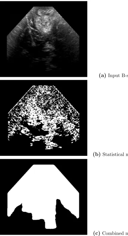
In figure 5, two methods were first compared. The first one is the solely sta-tistical approach: after the estimation of the noise model (parameter σ), each point x is tested as a shadow candidate by performing the test in equation 4 on a local square neighborhood of size 5 × 5 around x. The result of this sta-tistical approach is shown in figure 5-(b) and demonstrates that the stasta-tistical test is able to capture acoustic shadows, as well as hypoechogeneic areas. The combination of the geometrical method with the statistical test of eq. 4 ap-plied to Fig. 5-(a) leads to a more consistent detection of acoustic shadows as

seen in Fig. 5-(c). Due to the line sampling according to the probe’s geometry, only deep areas corresponding to shadows are detected.

4.3 Detection of acoustic shadows

The regularization effect is illustrated on intraoperative brain ultrasound im-ages, with 4 B-scans taken at 4 consecutive time stamps (figures 6-a-d). Differ-ent results were obtained with these four consecutive B-scans: without regu-larization in figures 6-(e-h), with 2D reguregu-larization (see figures 6-i-l) and with 2D + t regularization (see figures 6-m-p). For legibility purposes, only a few sampling lines were drawn.

The 2D regularization removed aberrant false positive detections like the dark red area on Figure 6-(m) corresponding to anatomical structures and smoothed the shape of the detected shadows. With the 2D+t regularization, the smooth-ing effect is stronger and there is more consistency from slice to slice. Regions of acoustic shadow and strong signal attenuation were detected by the method.

Typically, 400 scan lines were triggered for each image. The number of detected ruptures varies depending on some parameters. In our experience, we have found that it is better to detect and test many ruptures. Depending on the data, there is usually more than 50 ruptures tested per scan line. With the current sub-optimal implementation, the computation time is around 1 minute for a sequence of 50 B-scans.

4.4 Comparison with manually delineated ROI

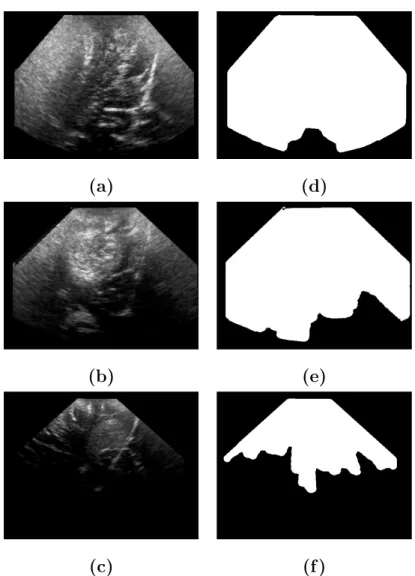
Since the automatic method detects both the B-scan geometry and the shadows as shown in figure 5-c, the image ROI (i.e., the B-scan mask without the detected shadows) was compared to a manual delineation of this area. Three real intraoperative sequences were chosen for this experiment, with depth varying from superficial ac-quisition 7-(a) to deep acac-quisition 7-(c). The extent of the acoustic shadows and signal attenuation increases with the acquisition depth.

Four experts manually delineated the areas using the ITKsnap soft-ware [18]. The corresponding segmentations are presented in Fig. 8. Visually, the experts segmentations exhibit very large differences. This fact supports the use of an objective automatic process to de-linetate these areas. As an evaluation criterion, the Dice coefficient, as well as the specificity and sensitivity were compared between the automatic method and the manual raters. Results are given in

Ta-bles 1, 2 and 3. Results show that the automatic method is very consistent with respect to the raters segmentations.

Rater 2 Rater 3 Rater 4 Automatic method

Rater 1 0.980 (0.96/0.99) 0.969 (0.94/0.98) 0.967 (0.97/0.93) 0.977(0.96/0.98) Rater 2 0.981 (0.97/0.98) 0.974 (0.99/0.91) 0.986 (0.97/0.96)

Rater 3 0.964 (0.99/0.87) 0.978 (0.99/0.92)

Rater 4 0.975 (0.98/0.93)

Table 1

Comparison between the various segmentations (manual raters, and automatic method) for the superficial dataset (7-(a)). For each comparison, the first figure is the Dice coefficient, followed the sensitivity and specificity into brackets. The au-tomatic method leads to results as consistent as the manual raters with an excellent detection rate.

Rater 2 Rater 3 Rater 4 Automatic method

Rater 1 0.964 (0.96/0.97) 0.936 (0.88/0.99) 0.958 (0.95/0.96) 0.933 (0.87/0.99) Rater 2 0.943 (0.89/0.99) 0.977 (0.97/0.97) 0.939 (0.88/0.99)

Rater 3 0.945 (0.99/0.86) 0.976 (0.97/0.96)

Rater 4 0.942 (0.99/0.86)

Table 2

Comparison between the various segmentations for the medium depth dataset (7-(b)) as in Table 1. The automatic method leads to results as consistent as the manual raters with an excellent detection rate.

Rater 2 Rater 3 Rater 4 Automatic method

Rater 1 0.855 (0.77/0.99) 0.781 (0.56/0.99) 0.819 (0.78/0.96) 0.817 (0.69/0.99) Rater 2 0.822 (0.70/0.99) 0.848 (0.91/0.94) 0.897 (0.83/0.98)

Rater 3 0.752 (0.99/0.84) 0.879 (0.98/0.91)

Rater 4 0.840 (0.73/0.99)

Table 3

Comparison between the various segmentations for the large depth dataset (7-(c)) as in Table 1. The Dice coefficient decreases compared to superficial acquisitions, since the relative size of the ROI compared to the image size decreases.

4.5 Impact on Reconstruction

The reconstruction of the non uniformly distributed set of B scans into a reg-ular 3D array of voxels is necessary for the successive processing steps like

registration and segmentation. Therefore reconstruction artifacts and image distortions must be avoided to ensure optimal image quality. To solve this problem, the reconstruction method presented in [14] was used. In this exper-iment, the data were composed of two sweeps from two view points that differ mostly by a translation. After application of the processing described above, areas detected as shadows regions were ignored in the distance-weighted in-terpolation step.

Figure 9-(a) shows a slice of the initial reconstruction and 9-(b) is the re-constructed slice when taking into account the detection of acoustic shadows. Figure 9-(c) shows the corresponding pre-operative MR slice. Artifacts are vis-ible, not only at the border between the two views, but also in deep regions. For instance, deep cerebral structures previously difficult to make out (lenticular nucleus and choroid plexus, see arrows) are clearly visible on the reconstructed US image when taking into account acoustic shadows. As a numerical assess-ment, the correlation ratio [15] was computed between the reconstructed US and the pre-operative MR. The correlation ratio increases from 0.15312 to 0.173996 when taking into account shadows, indicating objectively that the 3D reconstruction was improved.

4.6 Impact on registration

Registration of 3D ultrasound volumes is mandatory for quantitative image analysis and guidance [16, 17]. Registering ultrasound data is particularly needed in various situations: rigid registration of ultrasound data acquired at different surgical steps (e.g., before and after dura opening), registration of data for compounding purposes acquired from different view points or at different depths. It is expected that imaging artifacts such as acoustic shad-ows might adversely affect the registration process. Therefore, the benefit of removing detected acoustic shadows from the registration similarity is inves-tigated in this section. Using masks to select relevant voxels, the similarity based on the SSD (sum of square differences) for a given transformation T reads as: SSD(T ) =    R

(IM ask− JM ask◦ T )2 if IM ask∩ JM ask◦ T 6= ∅

+∞ if IM ask∩ JM ask◦ T = ∅

(5)

where IM ask and JM ask◦ T denote the reference masked image and the

trans-formed masked floating image. The registration similarity is based on the sum of square differences with a simplex optimization within a multiresolu-tion scheme. A barrier cost is included in the cost funcmultiresolu-tion in order to remove divergent solutions presenting no mask overlap.

In this section, three registration methods will be compared:

Method R : This registration is the standard registration with the SSD cri-terion on the entire image.

Method RG : This registration method accounts for the B-scan geometry and uses the B-scan mask as explained in equation (5).

Method RGASD : This registration method accounts for both the B-scan geometry and the acoustic shadows detection. The total mask is then used with the modified SSD criterion of equation (5).

To register two intraoperative sequences (i.e., to acquisitions at two depths), the transformation provided by the neuronavigation system can be used to assess registration methods. This transformation was used as a ground truth to assess the transformation resulting from the methods R, RG and RGASD. Here it was assumed that the coordinates given by the neuronavigation sys-tem were reliable: that was checked by visual inspection on salient structures. We considered two US sequences Iref and If lo registered together with the

transformation from the neuronavigation system Tneuro. To gather

registra-tion performance over a large number of samples and compute statistics, 100 random transformations Tn were applied to Iref. If lo was then registered and

the resulting transformation was then compared to the reference Tn◦ Tneuro

with the Frobenius matrix norm (||A||F = q

T r(AAH_))).

A set of 100 random rigid transformations was used in this framework, with translation and rotation parameters uniformly distributed in [-20;20]mm and [-20;20]° respectively. Two acquisitions from the same patient taken at the same surgical time (before dura opening) but at two different depths were selected as shown in Table 4 : deep (8cm) and middle deep (6cm) sequences were selected for Iref and If lo to get relevant areas of acoustic shadow.

Acquisition Sequence 1 - If lo Sequence 2 - Iref

Depth 6cm 8cm

Acoustic Shadow Ratio 13% 31%

Table 4

Ultrasound sequence characteristics : deep (8cm) and middle deep (6cm) sequences were selected for Iref and If lo with acoustic shadow ratio of 31% and 13%

respec-tively.

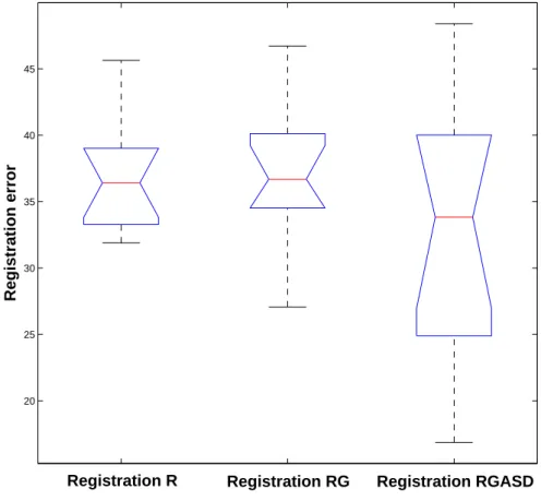
The Frobenius norm threshold used for the convergence rate estimation was set to 50. Above this value, all the registrations were showing visually aberrant results. The three methods are similar in terms of convergence for the first set of transformations as shown in Table 5. However, with the set of larger transformations, we notice an accuracy improvement when using the acoustic shadow information. The median and the upper bound of the distribution of registrations are very close, but there is a difference in the lower part of the

box plot in Figure 11 for the registration RGASD. This difference is confirmed by the computation of the mean of the distribution : the improvement is about 2mm and 2° closer to the ground truth on each parameter.

Registration method R RG RGASD

Convergence Rate 13% 12% 12%

Mean Error (Frobe-nius norm)

36 36 33,2

Table 5

Convergence Rate and Mean Errors computed with the Frobenius matrix norm. The introduction of acoustic shadows improves the registration accuracy.

5 Conclusion

In this paper, an automatic method to detect shadows in ultrasound images that uses image statistics and regularization for accurate detection of shadow borders was presented. The method was successfully tested on real intra-operative brain images, exhibiting a robust and reliable detection of acous-tic shadows when compared to a manual delineation of these shadows. It was shown that the incorporation of acoustic shadows in the reconstruction process improves the quality of the reconstruction. Thanks to a modified simi-larity criterion that incorporates the detected mask, the benefit of accounting for acoustic shadows in a registration task was assessed: it was shown that incorporating acoustic shadows in the process enables more successful regis-trations, down to sub-voxel accuracy. Therefore, we advocate that accounting for shadows and attenuation is important for accurate registration of intra-operative brain images. Incorporating acoustic shadows into the registration process leads to a slight increase in computational time that can be neglected compared to that required for the registration process. Finally, the inter-rater variability of the manually defined masks sen in Fig. 8 demonstrates the need for an objective automatic procedure to detect acoustic shadows as that pre-sented here.

In this paper, only a subset of acoustic shadows are detected corresponding to deep areas. Further work should focus on acoustic shadows that do not occur in deep zones, but revealing a reflectance interface like a gallstone. The framework presented here would need to be adapted to this case. For instance, the statistical detection test could be done after each rupture and between all following ruptures. In addition, more regularization constraints are needed to address concerns of minimum size and shape regularity. Further work should focus on the validation of such methods on various data including various types of shadows: air interfaces, bone interfaces, gallstones. For instance, the

detection of bone interfaces in ultrasound images may be of interest for the registration of such data to CT images.

References

[1] R. Steel, T. L. Poepping, R. S. Thompson, C. Macaskill, Origins of the edge shadowing artefact in medical ultrasound imaging, Ultrasound in Medicine & Biology 30 (9) (2004) 1153–1162.

[2] K. Drukker, M. L. Giger, E. B. Mendelson, Computerized analysis of shadowing on breast ultrasound for improved lesion detection, Medical Physics 30 (7) (2003) 1833–1842.

[3] D. Timmerman, A. C. Testa, T. Bourne, L. Ameye, D. Jurkovic, C. Van Holsbeke, D. Paladini, B. Van Calster, I. Vergote, S. Van Huffel, L. Valentin, Simple ultrasound-based rules for the diagnosis of ovarian cancer, Ultrasound in Obstetrics and Gynecology 31 (6) (2008) 681–690.

[4] A. Bekos, M. Arvaniti, K. Hatzimouratidis, K. Moysidis, V. Tzortzis, D. Hatzichristou, The natural history of peyronie’s disease: An ultrasonography-based study, European Urology 53 (3) (2008) 644–651.

[5] E. M. Caoili, B. S. Hertzberg, M. A. Kliewer, D. DeLong, J. D. Bowie, Refractory shadowing from pelvic masses on sonography: A useful diagnostic sign for uterine leiomyomas, Am. J. Roentgenol 174 (1) (2000) 97–101.

[6] A. Leroy, P. Mozer, Y. Payan, J. Troccaz, Rigid registration of freehand 3d ultrasound and ct-scan kidney images, in: C. Barillot, D. Haynor, P. Hellier (Eds.), Medical Image Computing and Computer Assisted Intervention, No. 3216 in LNCS, Springer-Verlag Berlin Heidelberg, St-Malo, 2004, pp. 837–844. [7] G. Penney, J. Blackall, M. Hamady, T. Sabharwal, A. Adam, D. Hawkes, Registration of freehand 3d ultrasound and magnetic resonance liver images, Medical Image Analysis 8 (2004) 81–91.

[8] A. Madabhushi, P. Yang, M. Rosen, S. Weinstein, Distinguishing Lesions from Posterior Acoustic Shadowing in Breast Ultrasound via Non-Linear Dimensionality Reduction, Engineering in Medicine and Biology Society, 2006. EMBS’06. 28th Annual International Conference of the IEEE (2006) 3070–3073. [9] X. Hao, S. Gao, X. Gao, A novel multiscale nonlinear thresholding method for ultrasonic speckle suppressing, IEEE Transactions on Medical Imaging 18 (9) (1999) 787–794.

[10] K. Krissian, K. Vosburgh, R. Kikinis, C.-F. Westin, Speckle-contrained anisotropic diffusion for ultrasound images, in: Proceedings of IEEE Computer Society Conference on Computer Vision and Pattern Recognition, San Diego CA US, 2005, pp. 547–552.

[11] P. Coup´e, P. Hellier, C. Kervrann, C. Barillot, NonLocal Means-based Speckle Filtering for Ultrasound Images. IEEE Transactions on Image Processing, 18 (10) (2009) 2221–2229.

[12] T. Loupas, W. N. McDicken, P. L. Allan, An adaptive weighted median filter for speckle suppression in medical ultrasonic images, IEEE transactions on Circuits and Systems 36 (1) (1989) 129–135.

[13] K. Hirakawa, T. W. Parks, Image denoising using total least squares, IEEE Transactions on Image Processing 15 (9) (2006) 2730–2742.

[14] P. Coup´e, P. Hellier, X. Morandi, C. Barillot, Probe trajectory interpolation for 3d reconstruction of freehand ultrasound., Medical Image Analysis 11 (6) (2007) 604–615.

[15] A. Roche, G. Malandain, N. Ayache, Unifying maximum likelihood approaches in medical image registration, International Journal of Imaging Systems and Technology: Special Issue on 3D Imaging 11 (1) (2000) 71–80.

[16] P. Coup´e, P. Hellier, X. Morandi, C. Barillot, A probabilistic objective function for 3d rigid registration of intraoperative us and preoperative mr brain images, in: IEEE International Symposium on Biomedical Imaging: From Nano to Macro, 2007.

[17] I. Pratikakis, C. Barillot, P. Hellier, E. M´emin, Robust multiscale deformable registration of 3D ultrasound images, International Journal of Image and Graphics 3 (4) (2003) 547–566.

[18] P.A. Yushkevich, J. Piven, H.C. Hazlett, R.G. Smith, S. Ho, J.C. Gee, and G. Gerig, User-guided 3D active contour segmentation of anatomical structures: Significantly improved efficiency and reliability, Neuroimage 31 (3) (2006):1116-28.

(a) Input B-scan

(b)Statistical method

(c)Combined method

Fig. 5. Effects of the statistical test and the geometrical constraint. (a): Intraop-erative 2D US of a left frontal glioma. In (b), black pixels represent the centers of patches detected as shadows with the statistical test only. Figure (c) presents the result obtained when combining the statistical and geometrical method. The introduction of a geometrical constraint leads to a more accurate and consistent detection of shadows.

(a) Initial (b) Initial (c) Initial (d) Initial

(e) Raw (f ) Raw (g) Raw (h) Raw

(i) 2D (j) 2D (k) 2D (l) 2D

(m) 2D + t (n) 2D + t (o) 2D + t (p) 2D + t

(m) at time t (n) at time t + 1 (o) at time t + 2 (p) at time t + 3

Fig. 6.Example of shadow estimation on intraoperative brain ultrasound images. For legibility, only a few lines were sampled in this case. Figures (a-d) show the initial B-scans, different results were obtained: without regularization (e-h), with 2D regularization (i-l) and with 2D + t regularization (m-p). The 2D regularized lines in red are overlaid on the 2D + t regularized lines in white for comparison. The 2D regularization removes outliers and smoothes the profile of the shadow boundaries. With the 2D + t regularization the

(a) (d)

(b) (e)

(c) (f )

Fig. 7. Left: Real intraoperative data used for the comparison with manual delin-eation. Data was chosen so as to represent three different depth acquisition: superfi-cial, medium and deep. Right: the corresponding ROI detected with the automatic method.

(Expert 1) (Expert 2) (Expert 3) (Expert 4)

(Expert 1) (Expert 2) (Expert 3) (Expert 4)

(Expert 1) (Expert 2) (Expert 3) (Expert 4)

Fig. 8. Expert segmentation of the image ROI for the dataset 7-(a) (top row), 7-(b) (middle row) and 7-(c) (bottom row). Despite reasonably high kappa values, the manual segmentation are visually significantly different, what advocates for an automatic process.

(a) Initial (b) Corrected (c) MR slice

Fig. 9. Impact of the shadow estimation on the reconstruction of 3D intraoperative brain ultrasound images. A sequence of 3D freehand ultrasound was acquired dur-ing brain surgery. Durdur-ing the sequence, two sweeps were done with different viewdur-ing angles. The two sweeps are compounded in one reconstructed volume and can be compared to the preoperative MR image (c). Image (a) shows a slice of the recon-structed volume with a Distance-Weighted reconstruction method. Reconstruction artifacts are visible on the boundaries of anatomical structures (sulci and cerebral falx). When incorporating the shadow estimation mask (figure (b)), artifacts are removed and deep structures appear clearly (lenticular nucleus and choroid plexus, see arrows). The ”border artifacts” at the left and right of the image are due to the B-scan mask that has been taken into account when reconstructing image (b).

(a)Sequence 1 - If lo (b) Sequence 2 - Iref

Middle deep acquisition (6cm) Deep acquisition (8cm) Fig. 10. 2D slices of the ultrasound sequences selected for the validation, after 3D reconstruction. An important acoustic shadow area can be observed at the bottom of the B-scan of Figure (b), due to the shadowing effect of the tumor and the cerebral falx.

20 25 30 35 40 45 Registration error

Registration R Registration RG Registration RGASD

Fig. 11. Box plot of the registration errors computed with the Frobenius matrix norm. From left to right : standard Registration (R), Registration working only on the B-scan Geometry mask (RG) and Registration that accounts for B-scan Geometry and Acoustic Shadows Detection (RGASD) The upper bound of the distribution is globally the same for all methods, but the mean value and the lower part of the box plot of the RGASD method shows an improvement in accuracy.