ÉCOLE DE TECHNOLOGIE SUPÉRIEURE UNIVERSITÉ DU QUÉBEC
ON THE CHARACTERIZATION OF JOHNSON-COOK CONSTANTS: NUMERICAL AND EXPERIMENTAL STUDY OF HIGH SPEED MACHINING AEROSPACE
ALLOYS
BY Monzer DAOUD
MANUSCRIPT-BASED THESIS PRESENTED TO ÉCOLE DE TECHNOLOGIE SUPÉRIEURE IN PARTIAL FULFILLMENT FOR THE DEGREE
OF DOCTOR OF PHILOSOPHY Ph.D.
MONTREAL, NOVEMBER 16TH, 2016
© Copyright
Reproduction, saving or sharing of the content of this document, in whole or in part, is prohibited. A reader who wishes to print this document or save it on any medium must first obtain the author’s permission.
BOARD OF EXAMINERS THIS THESIS HAS BEEN EVALUATED BY THE FOLLOWING BOARD OF EXAMINERS
Mr. Jean François CHATELAIN, Thesis Supervisor
Department of Mechanical Engineering at École de technologie supérieure
Mr. Abdel-Hakim BOUZID, Thesis Co-supervisor
Department of Mechanical Engineering at École de technologie supérieure
Mr. Roland MARANZANA, Chair, Board of Examiners
Department of Automated Manufacturing Engineering at École de technologie supérieure
Mr. Tan PHAM, Member of the jury
Department of Mechanical Engineering at École de technologie supérieure
Mr. Guénaël GERMAIN, External Evaluator
Department of Mechanical Engineering at École Nationale d'Arts et Métiers (ENSAM), France
THIS THESIS WAS PRESENTED AND DEFENDED IN THE PRESENCE OF A BOARD OF EXAMINERS
ON OCTOBER 20TH, 2016
ACKNOWLEDGMENTS
First of all I would like to express my sincere gratitude and deep appreciation to my supervisor professor Jean-François CHATELAIN and Co-supervisor professor Abdel-Hakim BOUZID for their helpful guidance, indispensable advice, and continuous help through the course of this thesis.
I am also extremely grateful to Prof. Souheil-Antoine TAHAN for his invaluable scientific advice and friendship.
I also would like to thank the jury members, Prof. Roland MARANZANA, Prof. Tan PHAM, and Prof. Guénaël GERMAIN for having accepted to evaluate my thesis and for their constructive comments.
I’m also grateful to all stuff at the machine shop, especially Éric MARCOUX, for all technical help and support during the experimental tests.
Special thanks go to my colleagues and friends at École de technologie supérieure for their friendships.
Finally, I would like to express my heartfelt gratitude for my parents, my sister, my brothers, and my wonderful wife for their endless love and encouragement.
ON THE CHARACTERIZATION OF JOHNSON-COOK CONSTANTS: NUMERICAL AND EXPERIMENTAL STUDY OF HIGH SPEED MACHINING
AEROSPACE ALLOYS Monzer DAOUD
RÉSUMÉ
L’industrie aéronautique souhaiterait à terme remplacer l’usinage chimique par l’usinage mécanique lequel est plus précis, plus prévisible et surtout plus écologique. En effet, les rejets issus de l’usinage chimique contiennent notamment du dioxyde de carbone et des solvants qui se dégradent difficilement dans les eaux souterraines. L’usinage mécanique permet aussi d’éviter une disposition importante de matières dangereuses et offre un meilleur recyclage des copeaux. Cependant, la maîtrise de la qualité des pièces produites par usinage mécanique, passe par la prédiction et l’optimisation du processus de coupe du métal. L’outil de simulation le plus utilisé est la modélisation par éléments finis (MÉF). La réussite et la fiabilité des modèles simulés dépendent fortement des lois décrivant le comportement thermomécanique des matériaux usinés. Parmi elles, la plus utilisée est celle de Johnson-Cook (JC), qui combine l'effet de la déformation, de la vitesse de déformation, et de la température. La détermination des paramètres constitutifs de JC pour des conditions d’usinage extrêmes (grande déformation, vitesse de déformation élevée, haute température) a longtemps été un défi majeur, mais une nécessité pour ceux qui appliquent la méthode des éléments finis pour modéliser la coupe à l’échelle de la formation des copeaux.
Cette étude a pour objectif de traiter cette problématique en tentant de mieux comprendre l'effet de la loi de comportement de JC sur la prédiction des paramètres de coupe (les efforts de coupe, les contraintes résiduelles, etc.) pour des alliages d’aluminium. Aussi dans le but de répondre aux besoins de l’industrie aéronautique, nous avons choisi des alliages d’aluminium (Al2024-T3, Al6061-T6, et Al7075-T6) couramment utilisés par celle-ci.
Ce travail de recherche est divisé en trois étapes successives.
Dans un premier lieu nous proposons une nouvelle approche d’identification des paramètres constitutifs de JC pour la coupe de métal. Celle-ci est basée sur la méthode inverse (tests d’usinage orthogonal) et la méthodologie de surface de réponse ce qui permet de générer un grand nombre de conditions de coupe pour une plage fixe de vitesse de coupe et d’avance, et de l'angle de coupe. Grâce à cette approche, nous avons pu analyser la sensibilité des paramètres constitutifs de JC à différents angles de coupe pour les trois alliages. Il a été constaté que, pour ces trois alliages cités, l’un des ensembles de paramètres constitutifs trouvés permet des prédictions plus précises de la contrainte d’écoulement par rapport à ceux rapportés dans la littérature. De plus, une étude par éléments finis en 2D de la coupe orthogonale a également montré une bonne corrélation entre les paramètres de coupe prédits
(efforts de coupe et épaisseur de copeau) et ceux obtenus expérimentalement lors de l’utilisation des paramètres constitutifs de JC identifiés par l’approche proposée.
En second lieu, nous avons prêté une attention particulière sur l’effet de l’angle de coupe sur les paramètres constitutifs de JC et par conséquent sur la prédiction des paramètres de coupe (les efforts de coupe, la morphologie de copeaux, la longueur de contact outil-copeau). Pour cela, différents ensembles de paramètres constitutifs de JC déterminés à différents angles de coupe (-8°, -5°, 0°, +5°, et +8°) ont été utilisés dans un modèle numérique d’éléments finis 2D pour simuler le comportement d’usinage de l’alliage Al2024-T3. Nous avons constaté que l’ensemble de paramètres constitutifs obtenu avec un angle de coupe de 0° donne globalement des prédictions plus précises des paramètres de coupe comparativement aux autres angles de coupe étudiés.
Enfin, la dernière étape de cette thèse est consacrée à la prédiction des contraintes résiduelles générées dans la pièce usinée (Al2024-T3) et des températures dans l’outil de coupe (uncoated carbide). Ainsi cette fois, nous avons décidé de considérer trois ensembles en se basant sur les résultats obtenus lors de l’étape précédente avec les angles de coupe de -8°, 0°, et +8°. Deux modèles numériques basés sur la méthode des éléments finis ont été utilisés: le premier été utilisé pour faire une analyse thermomécanique-2D pour simuler la coupe et le second pour une analyse thermique-3D pour étudier la distribution des températures. Les résultats montrent qu'une meilleure prédiction des contraintes résiduelles est obtenue lors de l'utilisation de JC à 0 ° tandis que les autres ensembles de JC à -8 ° et à + 8 ° ont tendance à respectivement surestimer ou sous-estimer celles-ci. Concernant la température dans l’outil de coupe, afin d’en évaluer la meilleure prédiction nous avons calculé des moyennes de températures simulées dans les outils de coupe de chaque ensemble de JC étudié. Nous avons remarqué que ces moyennes sont très proches des températures mesurées expérimentalement (environ 5,5% de différence) et nous avons déduit que les ensembles de JC n’influent pas sur la prédiction des températures de coupe dans l’outil.
Mots-clés: usinage mécanique; loi de comportement de Johnson-Cook; MÉF; identification; méthode inverse; alliages d’aluminium.
ON THE CHARACTERIZATION OF JOHNSON-COOK CONSTANTS: NUMERICAL AND EXPERIMENTAL STUDY OF HIGH SPEED MACHINING
AEROSPACE ALLOYS Monzer DAOUD
ABSTRACT
The aerospace industry would eventually replace chemical machining by mechanical machining which is more accurate, more predictable and more ecological. In fact, the discharges in the case of chemical machining contain especially carbon dioxide and solvents that are difficult to degrade in groundwater. The mechanical machining also avoids an important quantity of hazardous substances and provides better chips recycling. However, the control of mechanical machined parts quality goes through the prediction and the optimization of the metal cutting processes. The most attractive computational tool to predict and optimize metal cutting processes is the finite element modeling (FEM). The success and the reliability of any FEM depend strongly on the constitutive laws which describe the thermo-mechanical behavior of the machined materials. The most commonly used one is that of Johnson and Cook (JC) which combines the effect of strains, strain rates, and temperatures. The determination of the material constants of JC under high strains, strain rates, and temperatures during machining conditions has long been a major challenge but a necessity for those who apply finite element modeling techniques in machining processes at the chip formation scale.
This study aims at treating this subject in order to better understand the effect of the JC constitutive law on the prediction of cutting parameters (cutting forces, residual stresses, etc.) for aluminum alloys. In addition, in order to meet the interests of aerospace industry, three aluminum alloys (Al2024-T3, Al6061-T6 and Al7075-T6) commonly used in aircraft applications have been selected.
This research work is divided into three consecutive steps.
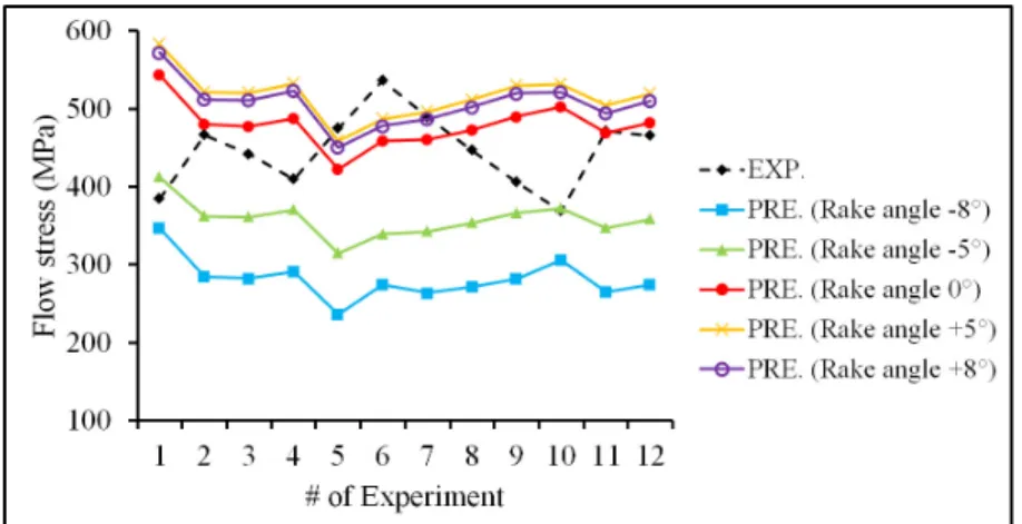
Firstly, a new approach to identify the material constants of JC for metal cutting is proposed. The approach is based on the inverse method (orthogonal machining tests) and the response surface methodology which allows generating a large number of cutting conditions within fixed ranges of cutting speed, feed rate, and rake angle. Based on this approach, the sensitivity of the material constants of JC to the rake angle for the three alloys was analysed. It was found that, for these three alloys, one set of the material constants obtained from the proposed approach predicts more accurate values of flow stresses as compared to those reported in the literature. Moreover, a 2D FEM investigation of the orthogonal cutting also showed a good agreement between the predicted cutting parameters (cutting forces and chip
thickness) and experimental ones when using the material constants obtained by the proposed approach.
Secondly, a specific focus was put on the influence of the rake angle on the material constants of JC and hence on the predicted cutting parameters (cutting forces, chip morphology, and tool-chip contact length). To achieve this goal, different sets of JC constants obtained at different rake angles (-8°, -5°, 0°, +5°, and +8°) were used in conjunction with a 2D finite element model to simulate the machining behavior of Al2024-T3 alloy. It was found that the material constants set obtained with 0° rake angle gives overall more accurate predictions of the cutting parameters as compared to other studied sets. Finally, the last step of this study is devoted to the prediction of induced residual stresses within the machined workpiece (Al2024-T3) and the temperature of the cutting tool (uncoated carbide). Three sets of JC based on the results obtained from the previous step with rake angles of -8°, 0°, and +8° were considered. Two finite element models were used; a 2D thermo-mechanical simulation to simulate chip formation and a 3D pure thermal analysis to obtain the temperature distribution. The results show that a better prediction of the residual stresses is obtained with JC at 0° while the other sets of JC at -8° and +8° tend to overestimate or underestimate the measured residual stresses, respectively. As far as the temperature of the cutting tool is concerned, the average values of the predicted temperatures of the cutting tool for each studied set of JC was considered in order to evaluate the best prediction. Based on these average values, the effect of the three sets of JC was not significant since the difference between the measured temperatures and the predicted average ones are less than 5.5% with the three cutting conditions.
Keywords: mechanical machining; Johnson-Cook constitutive law; FEM; identification, inverse method, aluminum alloys.
TABLE OF CONTENTS
Page
INTRODUCTION ...1
CHAPTER 1 RESEARCH OBJECTIVES AND THESIS OUTLINE ...13
Research objectives ...13
Thesis outline ...14
CHAPTER 2 LITERATURE REVIEW ...17
2.1 Introduction ...17
2.2 Residual stresses induced by the machining process ...17
2.2.1 Residual stress measurement techniques ... 20
2.2.2 Indirect methods... 20
2.2.3 Direct methods ... 21
2.2.4 In-depth residual stress measurement by X-ray ... 22
2.2.4.1 Analytical correction method of residual stresses ... 23
2.2.4.2 Finite element correction method ... 24
2.3 Cutting temperatures ...28
2.4 Finite element modeling considerations in metal cutting simulations ...31
2.4.1 Finite element formulations ... 31
2.4.2 Time integration methods ... 33
2.4.2.1 Mechanical analysis ... 33
2.4.2.2 Thermal analysis ... 37
2.4.3 Chip separation methods ... 38
2.4.4 Constitutive law models representing the flow stress for machining ... 39
2.4.5 Friction models ... 42
2.5 Applications of FEM in simulation of metal cutting ...44
2.6 Summary and conclusive remarks ...50
CHAPTER 3 EXPERIMENTAL AND FINITE ELEMENT INVESTIGATIONS ...51
3.1 Experiments ...51
3.1.1 Orthogonal cutting tests ... 51
3.1.1.1 Design of cutting tests ... 51
3.1.1.2 Experimental details... 52
3.1.2 Measurements of the residual stress in the workpiece ... 56
3.2 Finite element modeling ...58
3.2.1 Finite element model for chip formation using Deform-2D ... 58
3.2.1.1 Finite element mesh ... 60
3.2.1.2 Boundary conditions ... 62
3.2.1.3 Chip formation ... 63
CHAPTER 4 A MACHINING-BASED METHODOLOGY TO IDENTIFY MATERIAL CONSTUTIVE LAW FOR
FINITE ELEMENT SIMULATION ...69
4.1 Abstract ...69
4.2 Introduction ...70
4.3 Methodology to determine material constants of Johnson-Cook ...72
4.4 Experimental details...75
4.5 Finite element model and parameters ...76
4.6 Experimental results...77
4.6.1 Second-order models ... 77
4.6.2 Effect of the rake angle on material constants ... 82
4.6.3 Verification of the proposed approach ... 86
4.7 Finite element validation ...89
4.7.1 Cutting forces ... 89
4.7.2 Chip morphology ... 89
4.8 Conclusions ...92
CHAPTER 5 EFFECT OF RAKE ANGLE ON JOHNSON-COOK MATERIAL CONSTANTS AND THEIR IMPACT ON CUTTING PROCESS PARAMETERS OF AL2024-T3 ALLOY MACHINING SIMULATION ...95
5.1 Abstract ...95
5.2 Introduction ...96
5.3 Identification procedure of material constants of Johnson-Cook ...98
5.4 Experimental setup...100
5.5 Finite element machining simulation ...101
5.6 Results and discussion ...106
5.6.1 Cutting forces ... 106
5.6.2 Chip thickness ... 109
5.6.3 Tool-chip contact length ... 112
5.7 Conclusions ...113
CHAPTER 6 PREDICTION OF RESIDUAL STRESSES AND TEMPERATURES GENERATED DURING AL2024-T3 CUTTING PROCESS SIMULATION WITH DIFFERENT RAKE ANGLE-BASED JOHNSON-COOK MATERIAL CONSTANTS ...115
6.1 Abstract ...115
6.2 Introduction ...116
6.3 Johnson-Cook constitutive law and identification approach ...119
6.4 Experiments ...121
6.4.1 Workpiece material ... 121
6.4.2 Machining set-up ... 121
6.4.3 Residual stress measurement ... 124
6.5.1 Finite element model for residual stress prediction using
Deform-2D ... 128
6.5.2 Finite element model for temperature prediction using Deform-3D ... 130
6.6 Results and discussion ...132
6.6.1 Residual stresses ... 132
6.6.2 Temperature in the cutting tool ... 140
6.7 Conclusions ...146
CONCLUSION ...147
CONTRIBUTIONS ...153
RECOMMENDATIONS ...155
APPENDIX I Finite element correction method for in-depth residual stress measurement obtained by XRD ...157
APPENDIX II Determination of the physical quantities in the primary shear zone ...163
LIST OF TABLES
Page
Table 0-1 Constitutive law models for machining simulation ...11
Table 3-1 Geometry and physical properties for the tool substrate (K68) ...53
Table 4-1 Central composite design matrix for orthogonal cutting experiments ...75
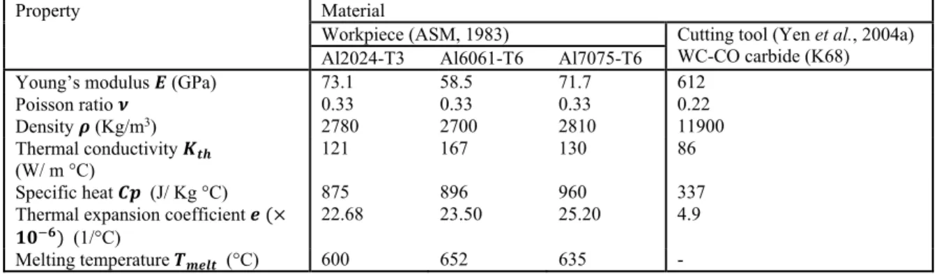
Table 4-2 Summary of physical properties for the tool substrate (K68) and workpiece material ...77
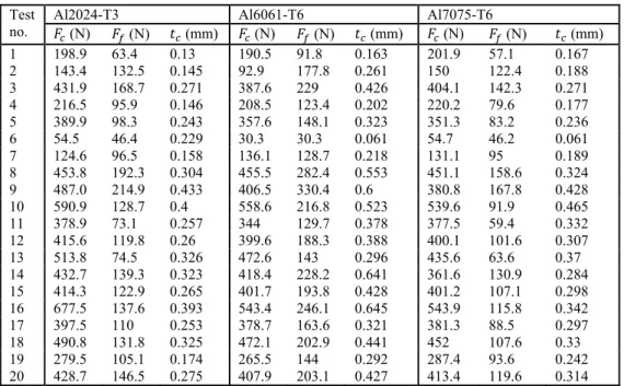
Table 4-3 Conditions and results of orthogonal cutting experiments performed on three aluminum alloys ...79
Table 4-4 Model parameters for Al2024-T3 ...79
Table 4-5 Model parameters for Al6061-T6 ...80
Table 4-6 Model parameters for Al7075-T6 ...80
Table 4-7 Material constants ...82
Table 4-8 Cutting test data for Al2024-T3 ( =0°) ...84
Table 4-9 Cutting test data for Al6061-T6 ( =0°) ...84
Table 4-10 Cutting test data for Al7075-T6 ( =0°) ...84
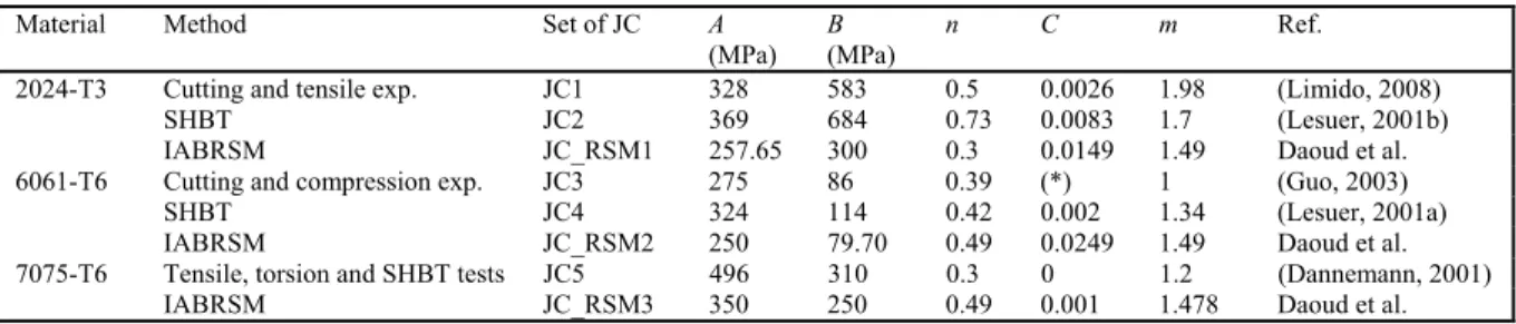
Table 4-11 Al2024-T3, Al6061-T6, and Al7075-T6 material constants obtained by different methods ...86
Table 4-12 Relative errors of the predicted flow stress ...87
Table 4-13 Comparison between experimental (EXP.) and predicted (FE) cutting forces ( =650 m/min, =0.16 mm/rev, =0°) ...90
Table 4-14 Comparison between experimental (EXP.) and predicted (FE) chip thickness ( =650 m/min, =0.16 mm/rev, =0°) ...92
Table 5-1 Material constants for Al2024-T3 ...99
Table 5-2 Physical properties of the workpiece material and the tool substrate (K68) ...103
Table 6-1 Material constants for Al2024-T3 identified (IDE.) at three rake angles ...120
Table 6-2 Cutting test data for Al2024-T3 ( =+5° & W=3.14 mm) ...120
Table 6-3 Geometrical position of the hole for embedded thermocouples ...124
Table 6-4 Cutting conditions ...124
Table 6-5 Parameters utilized in the X-ray measurements ...126
Table 6-6 Physical properties of the workpiece material and the tool substrate (K68) ...130
Table 6-7 Comparison between experimental results ( =950 m/min, =0.16 mm/rev) ...143
LIST OF FIGURES
Page
Figure 0-1 Basic terms in orthogonal cutting ...3
Figure 0-2 Configuration of the orthogonal cutting test and the direction of the cutting forces (a) disk-shaped workpiece (b) thin tube turning ...3
Figure 0-3 Orthogonal cutting configuration ...3
Figure 0-4 Deformation zones in orthogonal machining ...5
Figure 0-5 Classification of chip forms according to ISO 3685-1977 (E) ...5
Figure 0-6 Chip formation forms:(a) discontinuous, (b) elemental, (c) segmented, (d) continuous ...6
Figure 0-7 Shear plane model ...7
Figure 0-8 Slip line model ...8
Figure 0-9 Parallel-sided shear zone model ...9
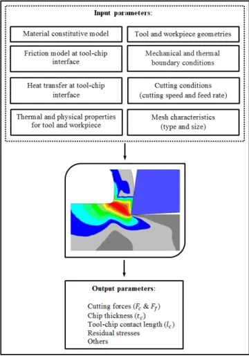
Figure 0-10 Main input parameters for FEM machining simulation ...10
Figure 2-1 (A) predominantly tensile plastic deformation (B) predominantly compressive plastic deformation ...19
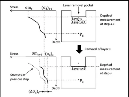
Figure 2-2 Schematic drawing of a layer removal process and a visualisation of the stress redistribution ...28
Figure 2-3 Representation of the Newton-Raphson method: (a) convergence (b) divergence ...36
Figure 2-4 Chip separation based on: (a) geometrical criterion (b) physical criterion ...39
Figure 2-5 Normal and frictional stress distribution according to (Zorev, 1963) ...44
Figure 3-1 Workpiece used in machining tests (dimensions are in mm) ...52
Figure 3-2 Measurement of cutting edge radius ...53
Figure 3-4 Fixture configuration ...54
Figure 3-5 Cutting and thrust forces in time domain ...55
Figure 3-6 Measurement of tool-chip contact length by optical microscope ...55
Figure 3-7 Circularity profile on the machined workpiece ...57
Figure 3-8 (a) Fixture configuration of the workpiece (b) Measurements of the residual stress using Proto iXRD machine (c) Measurements of removed layer thickness using Mitutoyo dial indicator ...57
Figure 3-9 Input and output parameters of the orthogonal machining modeling ...59
Figure 3-10 Initial workpiece and tool mesh configuration ...61
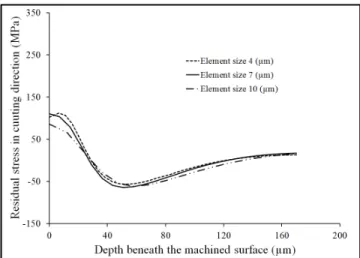
Figure 3-11 Mesh convergence within the uncut chip thickness ...61
Figure 3-12 Mesh convergence within the newly machined surface ...62
Figure 3-13 Kinematic boundary conditions of the workpiece and the tool ...62
Figure 3-14 Remeshing procedure: (a) Before remeshing (b) After remeshing ...63
Figure 3-15 Chip formation during orthogonal cutting simulation ...64
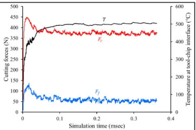
Figure 3-16 Cutting force, thrust force, and temperature versus time during orthogonal cutting simulation ...64
Figure 3-17 Comparison between predicted temperature and experimental one ( =950 m/min, =0.16 mm/rev, =0°) ...66
Figure 3-18 Mesh convergence (3D cutting tool modeling) ...67
Figure 4-1 Central composite design of experiment for three factors ...74
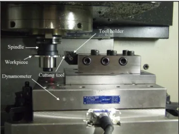
Figure 4-2 Experimental setup of the orthogonal cutting tests ...76
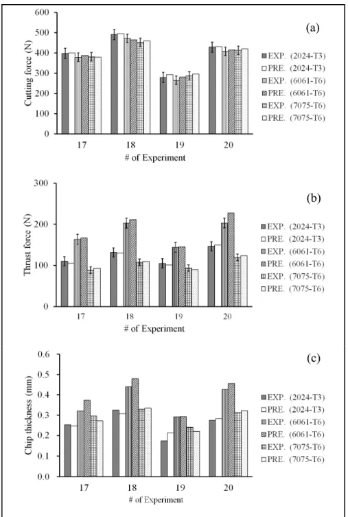
Figure 4-3 Comparison between the predicted and measured parameters: (a) cutting force, (b) thrust force, and (c) chip thickness ...81
Figure 4-4 Comparison of predicted flow stresses to the experimental data for Al2024-T3 ...85
Figure 4-5 Comparison of predicted flow stresses to the experimental data for Al6061-T6 ...85
Figure 4-6 Comparison of predicted flow stresses to the experimental data
for Al7075-T6 ...85
Figure 4-7 Comparison between experimental (EXP.) and predicted (PRE.) chip morphology for Al2024-T3 alloy ( =650 m/min, =0.16 mm/rev, =0°) (a) EXP., (b) PRE. By FE_JC1, (c) PRE. By FE_JC2, and (d) PRE. By FE_RSM1 ...91
Figure 4-8 Comparison between experimental (EXP.) and predicted (PRE.) chip morphology for Al6061-T6 alloy ( =650 m/min, =0.16 mm/rev, =0°) (a) EXP., (b) PRE. By FE_JC3, (c) PRE. By FE_JC4, and (d) PRE. By FE_RSM2 ...91
Figure 4-9 Comparison between experimental (EXP.) and predicted (PRE.) chip morphology for Al7075-T6 alloy ( =650 m/min, =0.16 mm/rev, =0°) (a) EXP., (b) PRE. By FE_JC5, and (c) PRE. By FE_RSM3 ...92
Figure 5-1 Inverse approach based on response surface methodology (IABRSM) ...99
Figure 5-2 Comparison between the five sets of JC: effect of rake angle ...100
Figure 5-3 Experimental setup utilized during the orthogonal cutting tests ...101
Figure 5-4 Displacement and thermal boundary conditions of the 2D FE model ...103
Figure 5-5 Influence of the temperature and strain on the material flow stress ( =105 s-1) (a) JC(-8°), (b) JC(-5°), (c) JC(0°), (d) JC(+5°), and (e) JC(+8°) ...105
Figure 5-6 Influence of the temperature and strain rate on the material flow stress ( =1.5) (a) JC(-8°), (b) JC(-5°), (c) JC(0°), (d) JC(+5°), and (e) JC(+8°) ...106
Figure 5-7 Variation of cutting forces with the cutting conditions during the experiments ...107
Figure 5-8 Comparison between experimental (EXP.) and predicted (FE. PRE.) tangential forces ...108
Figure 5-9 Comparison between experimental (EXP.) and predicted (FE. PRE.) thrust forces ...109
Figure 5-11 Comparison between experimental (EXP.) and predicted (FE. PRE.)
chip thickness ...111
Figure 5-12 Comparison between experimental (EXP.) and predicted (FE. PRE.) chip morphology for test no. 2. (a) EXP. (b) FE. PRE. JC(-8°), (c) FE. PRE. JC(-5°), (d) FE. PRE. JC(0°), (e) FE. PRE. JC(+5°), and (f) FE. PRE. JC(+8°) ...111
Figure 5-13 Comparison between experimental (EXP.) and predicted (FE. PRE.) Tool-chip contact length ...113
Figure 6-1 Comparison between experimental (EXP.) and predicted (PRE.) flow stresses (cutting conditions listed in Table 6-2) ...121
Figure 6-2 Orthogonal machining test (a) experimental setup (b) side view of the cutting components ...123
Figure 6-3 Time constant required to reach 63.2 % of the final temperature measurement ...123
Figure 6-4 Appearance of the blind hole made in the cutting insert by EDM ...123
Figure 6-5 Hole position inside the cutting insert for embedded thermocouple ...124
Figure 6-6 Experimental setup of the residual stress measurements ...125
Figure 6-7 Removing successive layers of material (a) Electro-polishing set-up (b) Measurements of removed layer thickness ...126
Figure 6-8 Circularity profile of the machined workpiece ...127
Figure 6-9 Initial boundary conditions of the 2D finite element model ...130
Figure 6-10 Flow chart of FEM for residual stress and temperature predictions ...131
Figure 6-11 3D finite element model and the thermal boundary conditions ...132
Figure 6-12 Experimental (EXP.) residual stresses distribution in cutting direction for Al2024-T3 ...134
Figure 6-13 Comparison between experimental (EXP.) and predicted (F.E. PRE.) residual stress profiles ...135
Figure 6-14 Effect of JC sets on equivalent plastic strain during cutting, ( =950 m/min, =0.16 mm/rev, =+8°) (a) JC(-8°) (b) JC(0°) (c) JC(+8°) ...136
Figure 6-15 Effect of JC sets on the material flow stress during cutting ...138 Figure 6-16 Effect of JC sets on temperature beneath the tool-tip during cutting ...139 Figure 6-17 Effect of JC sets on temperature at tool-chip interface during cutting ...141 Figure 6-18 Contact nodal temperature coming from 2D
thermo-mechanical simulations ...142 Figure 6-19 Predicted temperature distribution
( =950 m/min, =0.16 mm/rev, =-8°) ...143 Figure 6-20 Thermocouple positions selected inside the cutting tool ...144 Figure 6-21 Comparison between experimental (EXP.) and predicted (F.E. PRE.)
LIST OF ABREVIATIONS BUE Built-up edge
CCD Central composite design
CMM Coordinate measuring machine DOC Depth of cut
EDM Electrical Discharge Machine
FE Finite element
FEA Finite element analysis
FEM Finite element modeling
HSM High speed machining
IABRSM Inverse approach based on response surface methodology JC Johnson-Cook
M&E Moore and Evans RSM Response surface methodology SHBT Split-Hopkinson bar technique
LIST OF SYMBOLS AND UNITS OF MEASUREMENTS
, , Hole position parameters (mm) Yield strength coefficient (MPa) Hardening modulus (MPa)
Strain rate sensitivity coefficient (-) Heat capacity matrix (J/°C)
Specific heat of work material (J/Kg °C) Damage parameter (MPa)
DOC Depth of cut (mm)
E Young’s modulus (GPa)
e Thermal expansion coefficient (1/°C) , Tangential and thrust force components (N) Externally applied force vector (N)
Feed rate (mm/rev)
Nodal point residual force vector (N)
Residual function (N)
h Thickness of the primary shear zone (mm) ℎ Interface heat transfer coefficient (N/s mm °C) ℎ Convection heat transfer coefficient (N/ s mm °C)
I Identity matrix (-)
Thermal conductivity (W/m °C)
Shear flow stress in the chip at the tool-chip interface (MPa) Heat conduction matrix (W/°C)
k Independent variables
K Stiffness matrix (kg/s2)
Correction coefficient at depth “d” for the step “s” (-) Correction matrix (-)
Modified correction matrix (-) Tool chip contact length (µm) Thermal softening coefficient (-)
Shear friction coefficient (-) M Masse matrix (Kg)
Hardening coefficient (-)
N Number of data Heat flux vector (W)
Coefficient of determination (-)
Adjusted coefficient of determination (-)
, , Inner, outer, and actual measurement radius (mm) Temperature of the work material (°C)
Vector of nodal point temperatures (°C) Melting point of the work material (°C)
Room temperature (°C)
Average temperature on the primary shear plane (°C) Vector of nodal temperature rates (°C/s)
Chip thickness (mm) Displacement vector (m)
Acceleration vector (m/s2)
Cutting speed (m/min) Initial guess velocity (m/s) Width of cut (mm)
, Machining parameters (-) y Response surface (-)
Tool rake angle (°)
Angle of the inclination of the primary collimator (°) , , , Regression coefficients (-)
Deceleration coefficient (-) 2 Bragg angle (°)
Plastic equivalent strain on the primary shear plane (-) Equivalent strain rate on the primary shear plane (s-1)
Reference strain rate (s-1)
ε Effective strain (-)
Equivalent flow stress at the primary shear zone (MPa) Normal stress at tool-chip interface (MPa)
σ Maximum principal stress (MPa)
, , Corrected stress in radial, tangential, and axial directions (MPa) , Measured stress in tangential and axial directions (MPa)
Stress measured in the direction of interest on the top of the layer “s” (MPa) Stress measured in the direction of interest on the top of the layer “s+1” (MPa) ( ) , ( ) Stress at depth “d” after removing layers “s” and “s-1” (MPa)
Residual stress corrected for material removal at depth “d” (MPa) Residual stress measured at depth “d” without correction (MPa) (∆ ) Local stress variation at depth “d” after removal step “s” (MPa)
Column vectors of the corrected stresses (MPa) Column vectors of the measured stresses (MPa)
Average of two measured stresses on both side of the removed layer “s”(MPa) Column vector containing all the average measured stresses (MPa)
Frictional shear stress at the tool-chip interface (MPa) Coefficient of friction (-)
Poisson ratio (-) Density (kg/m3)
∆ Time step (s)
∆ Critical time step (s)
∆ Velocity correction term (m/s)
Experimental error of the observations (-)
Shear angle (°)
INTRODUCTION
Nowadays, the aeronautical industry is more and more interested in the use of conventional machining rather than the chemical machining in order to comply with the environmental protection laws and regulation and to enhance the functional behavior of the machined structural components.
The use of light weight structural materials with high strength is always in demand from the manufacturing industries. Aluminum alloys such as Al2024-T3, Al6061-T6, and Al7075-T6, which belong to this category, are widely utilized in the aeronautical industry. However, tendency of built-up edge (BUE) formation and unfavorable chips (such tangled and ribbon chips) are often encountered during the machining of theses alloys which can affect the surface finish, dimensional tolerances and tool life. In order to overcome these drawbacks, cutting fluids are often used. However, the coolants result in ecological and economic problems, consequently, there is an interest in dry high speed machining (HSM) to make this metal cutting as a green process as possible (Sreejith et Ngoi, 2000). Moreover, HSM has been reported as high material removal rates, enhancement in product quality as well as surface finish, and elimination of BUE and burrs (Fallböhmer et al., 2000; Rao et Shin, 2001).
In fact, machining is one of the most manufacturing processes widely used in industry. Machining is defined as the process in which unwanted material is carried away gradually from a workpiece. Cutting is a term that describes the formation of a thin layer, called chip, via the interaction of a wedge-shaped tool with the surface of the workpiece, given that there is a relative motion between them (Markopoulos, 2012). In most practical operations, the cutting tool is three-dimensional and geometrically complex. For this reason, the two-dimensional orthogonal cutting is used to explain the basic mechanism of metal cutting. In orthogonal cutting, which is the subject of the current research, the cutting edge of the tool is perpendicular to the cutting direction (primary motion), as shown in Figure 0-1. In addition,
orthogonal cutting could be assumed as plane strain condition if the following considerations are respected: (1) the cutting edge is straight and sharp and wider than the width of the machined workpiece. (2) the cutting edge of the tool is perpendicular to the cutting velocity. (3) the width of cut is larger than or equal to 10 times the uncut chip thickness.
Therefore, two cutting forces (cutting force and thrust force ) are identified in orthogonal cutting configuration, as shown in Figure 0-2. From the experimental point of view, the orthogonal cutting test can usually be carried out with two set-ups. In the case of turning a disk-shaped workpiece (Figure 0-2 (a)), the straight cutting edge is set parallel to primary rotation axis of the workpiece and is moved linearly towards the center of the disk (feed motion). Since the feed motion results in reduction of disk diameter, the cutting speed is kept constant by increasing the rotation speed. Thin tube turning is also used for orthogonal cutting tests, as shown in Figure 0-2 (b). Here, the cutting speed changes over the cutting edge. By choosing a tube with large diameter and thin wall thickness, the changing in cutting speed could be minimized. The literature review illustrates that the orthogonal cutting tests conducted using a disk-shaped workpiece represents more truly plane strain problem rather than the commonly used thin tube turning experiments due to the fact that chips curl always sideward and out of plane (Ee et al., 2005). Although these two set-ups satisfy the consideration mentioned above, nevertheless, they have two major disadvantages as the residual stresses analysis is considered: the first one is related to the choice of a machined surface zone which is representative of the cutting test and the second one is the effect of cutting passes during the machining tests. Recently (Ducobu et al., 2015) presented a simple set-up to perform orthogonal cutting experiments using a standard milling machine as a planning machine. In this set-up, the workpiece is inserted to the spindle and the tool is mounted on the tool holder. The cutting is achieved by moving the workpiece towards the stationary cutting tool at a cutting speed , as shown in Figure 0-3. The main drawback of this set-up is that the maximum cutting speed is limited to the maximum feed rate of the machine; therefore, this set-up cannot be used in HSM of aluminum alloy, for example. In addition, great care must be taken to position the cutting tool at a distance sufficient far from the workpiece in order to assure that the required cutting speed is reached before cutting.
Figure 0-1 Basic terms in orthogonal cutting (Astakhov, 2010)
Figure 0-2 Configuration of the orthogonal cutting test and the direction of the cutting forces (a) disk-shaped workpiece (Umbrello et al., 2007b)
(b) thin tube turning (Özel, 2003)
Figure 0-3 Orthogonal cutting configuration (Ducobu et al., 2015)
Figure 0-4 shows the chip formation obtained from FEM of orthogonal machining. As the wedge-shaped tool penetrates into the workpiece, the metal ahead of the tool tip undergoes a very high plastic deformation and it is sheared over the primary shear zone to form a chip. This chip (sheared material) slides up the tool face and is partially deformed under high normal stresses and friction resulting in a secondary deformation zone in which high temperature is generated. Tertiary shear zone is created due to the friction between the flank face of the tool and the newly machined surface. This friction area has no effect on the chip formation but it influences the machined surface.
Extreme conditions are encountered during machining tests which lead to different thermo-mechanical loads in the shear zones. Consequently, different types of chip forms are obtained. These chip forms were classified based on their geometrical appearance as depicted in Figure 0-5. Another possible classification was introduced in (Grzesik, 2008). In this case, the chips were classified into continuous, segmented, elemental, and discontinuous chips (see Figure 0-6). This classification is based on material deformation and relevant fracture mechanisms resulting from the interaction between cutting conditions and the workpiece properties. A discontinuous chip formation (Figure 0-6 (a)) happens when fracture occurs before complete chip plastic deformation takes place. An elemental chip (Figure 0-6 (b)) is characterized by variations in chip thickness in periodic manner formed under high speed and hard machining conditions. In segmented chips (Figure 0-6 (c)), the chip is characterized by areas having intense shear deformation (shear bands) separated by other areas with relatively lower deformation. In fact, under certain cutting conditions, the plastic strain rates become high enough to generate considerable heat in the primary shear zone which cannot rapidly be dissipated to the rest of workpiece material. This results in a quasi-adiabatic condition which causes material thermal softening (Xie et al., 1996). As the cutting process continues, the local strain increases until an instantaneous shearing takes place (Jawahir et Van Luttervelt, 1993). However, the explanation of segmented chip formation by adiabatic shear theory is not unanimously accepted and another explanation of segmented chip formation based on fracture theory is reported in the literature (Vyas et Shaw, 1999). Continuous chip formation
(Figure 0-6 (d)) takes place when the chip formation occurs without fracture on the shear plane.
It is worth pointing out that the classification of chip forms is highly important for the cutting machining modeling. Although the existence of various analytical and numerical models of chip formation, it is always difficult to predict an accurate chip shape generated for a set of cutting conditions. This could explain why most research work is limited to the modeling of the continuous chip formation.
Figure 0-4 Deformation zones in orthogonal machining
Figure 0-5 Classification of chip forms according to ISO 3685-1977 (E) Source: (Grzesik, 2008)
Figure 0-6 Chip formation forms:(a) discontinuous, (b) elemental, (c) segmented, (d) continuous (Grzesik, 2008)
The modeling of machining processes is highly important. It provides an understanding of the physics involved in the chip formation mechanism which in turns help design new geometry cutting tools, develop new machining alloys, and achieve effective optimization. Consequently, the traditional trial and error approach could be avoided.
Over the last decades, several analytical models of chip formation have been proposed by many researchers. The most widely known model for cutting is the shear plane developed by Ernst et Merchant (1941). In this model, the continuous chip formation is generated by a shearing process on a thin plane (plane AB in Figure 0-7), called shear plane. The shear stress is assumed to be independent of the shear angle and is distributed uniformly along the shear plane. The cutting velocity is instantaneously changed to the chip velocity across the shear plane. Figure 0-7 shows the condensed force diagram defining the relationship between the cutting force components during cutting. In the shear plane model, cutting force
and thrust force are determined if the shear angle ∅, friction angle , rake angle , shear stress , and uncut ship thickness , and the depth of cut are known.
Figure 0-7 Shear plane model Source: (Merchant, 1945)
Based on the assumption that the material will choose to shear at an angle that minimizes the required energy, the shear angle, angle between the shear plane and the cutting direction, is given by:
∅ =
4+2−2 (0-1)
Although there is a lack of agreement with experiment, the shear plane model is considered as a reference for other models that followed.
Lee et Shaffer (1951) developed a more advanced model based on the theory of slip line field to predict cutting forces, chip thickness, and shear angle from tool geometry, the friction coefficient, and the yield stress of the workpiece material. Similar to the shear plane model, the plastic deformation is assumed to take place on the shear plane AB, but the plastic field is extended above this plane to form a triangular plastic zone, as shown in Figure 0-8. The shear angle predicted by this model is given by:
∅ =
It was reported that this model did not significantly enhance the results as compared to the shear plane model and both models showed relatively poor agreement with experiments (Pugh, 1958). This poor accuracy could be explained by the fact that the effect of the temperature and the strain rate were neglected and a simple friction model was used in both above mentioned models.
Figure 0-8 Slip line model Adopted from (Lee et Shaffer, 1951)
Recently, Fang et al. (2001) developed a universal analytical predictive model for machining with a restricted contact grooved tools. This model integrates six representative slip line models developed for machining in the past five decades, namely the models of Dewhurst (1978), Lee et Shaffer (1951), Johnson (1962) and Usui et Hoshi (1963), Kudo (1965), Shi et Ramalingam (1993), and Merchant (1944). The major output parameters of the universal model include: cutting forces, chip thickness, chip up-curl radius, and chip back-flow angle. As reported by Fang et Jawahir (2002), the universal model follows two fundamental assumptions: (1) the rigid-perfectly plastic assumption in which no effects of strains, strain rates, and temperatures on the material shear flow stress is taken into consideration (2) plane strain deformation assumption.
Oxley et Young (1989) proposed more sophisticated model based on experimental observations. The shear angle is predicted based on the strain and strain rate by using the slip
line and parallel-sided shear zone theory. The average strain rate is modeled as a function of a constant shear velocity and the length of the shear plane. Oxley model permits the prediction of the cutting forces under the effect of the flow stress of the workpiece. In this model, two plastic zones, namely primary zone and secondary zone, are considered, as depicted in Figure 0-9. The average temperatures in the primary zone and at the tool-chip interface, due to the heat generation by the plastic deformation, were also derived.
Figure 0-9 Parallel-sided shear zone model Source: (Pittalà et Monno, 2010)
The above mentioned analytical models provide useful insight into the mechanics of the metal cutting.
More promising approach for studying metal cutting is provided by numerical techniques such as the finite element modeling (FEM). The flexibility of the finite element method allows it to deal with large deformation, strain rate effect, tool-chip contact and friction, local heating and temperature effect, different boundary and loading conditions, and other phenomena encountered in metal cutting problems (Shet et Deng, 2003).
Figure 0-10 outlines the main input parameters for FEM machining simulation. One of the most important governing parameter in any cutting simulation is the use of an accurate
constitutive law model which represents the material behaviour especially at the extreme conditions that exist in the shear zones (Childs, 1997; Sartkulvanich et al., 2005a; Shi, 2011).
Figure 0-10 Main input parameters for FEM machining simulation
Several constitutive law models that are adopted for machining simulation have been proposed to reproduce the thermo-mechanical effects involved in metal cutting, as listed in Table 0-1. Among these constitutive laws, the Johnson-Cook (JC) model has been widely used for machining simulation because it represents adequately the material flow stress of several metallic materials in terms of their strains, strain rates, and temperatures. Moreover, this constitutive law, available in many finite element codes, has been successfully used with aluminum alloy to predict the flow stress in conditions similar to metal cutting (Jaspers et Dautzenberg, 2002).
However, different constitutive model constants for the same material could be found in the literature which can affect significantly the predicted results of the machining process such as cutting forces, chip morphology, temperatures, tool wear, and residual stresses. These discrepancies could be attributed, principally, to the different methods used for the determination of the constitutive model constants. The literature review illustrates that most
common experimental methods used to identify constitutive law models are static tests (tensile, compression), dynamic tests (Split-Hopkinson bar technique; Taylor test), and inverse method (machining test). Sartkulvanich et al. (2005b) have attested that, in metal cutting simulation, material constants should be obtained at high strain rates (up to 106 s-1)
temperatures (up to 1000 °C), and strains (up to 4); therefore, the inverse method (machining test) which is conducted under these conditions has proven to be effective as a characterization test (Umbrello et al., 2007b).
As a result, a new approach to identify the material constants of the constitutive law based on orthogonal machining tests is investigated and aimed to provide more reliable material constants that can be used in FEM machining simulation.
Table 0-1 Constitutive law models for machining simulation
Constitutive law models Constitutive law equations constants References Johnson-Cook = + ( ) 1 + ln 1 − − − A, B, C, m, n (Johnson et Cook, 1983) Power law = ̅ , m, n, (Shi et Liu, 2004)
Vinh = ( ) exp , m, n, G (Vinh et al., 1979)
Zerilli-Armstrong For b.c.c. metal
= + exp − + + ( ) For f.c.c. metal = + ( )⁄ exp − + , , , , (Zerilli et Armstrong, 1987) Oxley = , ( ) , , , , (Oxley et Young, 1989) Marusich 1 + = if < 1 + 1 + = if > = 1 − ( − ) 1 + ̅ , , , , (Marusich et Ortiz, 1995)
CHAPTER 1
RESEARCH OBJECTIVES AND THESIS OUTLINE Research objectives
The determination of material flow stress constants under high strains, strain rates, and temperatures during machining conditions has long been a major challenge but a necessity for those who apply the finite element simulation modeling techniques for machining process development. As mentioned above, the different material constants provided in the literature for the same material are not reliable since they significantly affect the predicted results. It was shown that most of these parameters are reasonably predicted when using material constants obtained from machining tests. Unfortunately, a reduced number of machining experiments for the identification of the constitutive law have been used which can affect the optimization procedure. In addition, different rake angles were used during these machining tests to obtain the material constants. In fact, the chip formation mechanism could easily change from continuous to segmented chip when the rake angle changes from positive to negative values. These two mechanisms lead to different thermo-mechanical loads in the cutting zone. Thus, the rake angle appears to have a significant effect on the constitutive models when the inverse method is considered.
The overall objective of this research work is to cover this issue to comprehensively understand the effect of the material constitutive law on the predicted machining results.
In particular, the specific objectives of the proposed research are to:
i) Develop an experimental approach to identify the material constants of the JC constitutive law model for finite element modeling simulation of high speed machining in order to improve the existing inverse method;
ii) Investigate the effect of the rake angle on the material constants of the JC constitutive law model;
iii) Conduct a sensitivity analysis on the effect of the different sets of JC constitutive law material constants, identified at different rake angles, on the numerically predicted machining results in order to standardize the existing inverse method.
Thesis outline
This research work is presented as a thesis by publication and is divided into five chapters.
Chapter 2 provides an overview of the relevant works that have been achieved in the literature and it ends by a summary and a literature review in order to highlight the problem defining the scope of the present research.
Experimental and finite element details are presented in chapter 3.
Chapter 4 presents the first published journal article. In this research work, an inverse approach based on response surface methodology was developed to determine the material constants of Johnson-Cook. Three aluminum alloys (Al2024-T3, Al6061-T6, and Al7075-T6) were considered in order to cover a wide range of commercial aluminum alloys commonly used in aircraft applications. In addition, a particular focus was made to study the effect of the rake angle on the identification of the constitutive law. Finally, a FEM investigation was carried out to validate the obtained material constants.
From the above investigation, it was concluded that the rake angle has a significant effect on the constitutive model when the inverse method is considered. In this context, five sets of JC constitutive law determined at five different rake angles and obtained in the first article were employed to simulate the machining behavior of Al2024-T3 alloy using FEM. Therefore, the effects of these sets of JC constants on the numerically predicted cutting forces, chip
morphology, and tool-chip contact length were the subject of a comparative investigation of the second published journal article presented in chapter 5.
Finally, chapter 6 presents the third submitted journal article. In this work, the effect of different sets of JC constants on the numerically predicted residual stresses in the machined components of Al2024-T3 and cutting temperatures for the uncoated carbide tool were investigated. In this context, two different approaches are considered in this study. The former is a thermo-mechanical analysis using Deform-2D finite element software in order to predict the residual stresses induced in the workpiece. The latter is a pure thermal simulation using Deform-3D software to obtain the temperature distribution in the cutting tool.
The thesis conclusion drawn from the current research work and recommendations for future work are provided at the end of this thesis.
CHAPTER 2 LITERATURE REVIEW 2.1 Introduction
This chapter summarises the most important issues relevant to the current works. The first section is devoted to the machining-induced residual stresses: their importance, their definition, their possible sources, their classifications, the different experimental techniques used to measure them, and the subsurface residual stress measurements as well as the different techniques used to correct these measurements. The second section presents the cutting temperature and the most commonly experimental techniques for temperature measurements. The third section describes the main FEM aspects for metal cutting processes. This includes the presentation of different finite element formulations, the time integration methods for solving non-linear problems, the existing chip separation methods, and the modeling of both the workpiece material and the friction at tool-chip interface. The fifth section is devoted to the FEM of the metal cutting, underlying the main investigations that have been carried out in this regard. Finally, this chapter ends by providing the main finding in the literature including a review in order to highlight the problem defining the scope of the present research.
2.2 Residual stresses induced by the machining process
The functional behavior of a structural component is heavily influenced by the residual stress distribution caused by the machining process. It is known that fatigue life, deformation, static strength, chemical resistance, and electrical properties are directly influenced by the residual stresses (Brinksmeier et al., 1982; Capello, 2005; El-Axir, 2002; Young, 2005). It is therefore necessary to understand and control the residual stresses for the functionality and longevity of engineering structures.
The residual stresses are defined as those stresses that remain in the machined workpiece after machining is completed and a return to the initial state of temperature and loading is achieved. During machining, the formation of residual stresses is induced under the action of the three following mechanisms (Guo et Liu, 2002b):
• Mechanical deformation: non-uniform plastic deformation due to cutting forces; • Thermal deformation: non-uniform plastic deformation induced as a result of thermal
gradient;
• Metallurgical alterations: specific volume variation resulted from phase transformation.
It is worth mentioning that the first two mechanisms are always present and occur simultaneously in most cutting processes while the third one depends on the amount of heat generated during the cutting, as well as the cooling rate.
Mechanical deformation induced in superficial layer material due to the applied mechanical load may produce both tensile and compressive residual stresses (El-Wardany et al., 2000). In fact, the superficial layer material of the workpiece is subjected to loading cycles of stress versus strain along the cutting direction, as shown in Figure 2-1. The material element first experiences compressive plastic deformation ahead of the advancing cutting tool and then tensile plastic deformation behind it. As a result, this region is the seat of two consecutive modes of deformation and the predominant one, after cutting, determines the final state of residual stresses (Wu et Matsumoto, 1990). Since the superficial layer material is constrained by the bulk material beneath, surface compressive residual stress will be produced, after relaxation, if the loading cycles give rise to a tensile plastic deformation, and vice versa, as shown in Figure 2-1.
In dry cutting, the superficial layer material of the workpiece absorbs more heat and tends to elongate more than the bulk material beneath. After cutting, the hot superficial layer remains hot because the cooling starts mainly from the bulk material by conduction. Since its thermal
expansion is constrained by the bulk material beneath, large compressive stress is generated in the surface material. If this compressive stress exceeds the yield strength of the surface material, the superficial layer will plastically deformed under compression stress, which in turn, surface tensile residual stress is produced after cooling (El-Wardany et al., 2000; Shi et Liu, 2004).
Figure 2-1 (A) predominantly tensile plastic deformation (B) predominantly compressive plastic deformation
(Wu et Matsumoto, 1990)
As mentioned above, if the temperature induced during cutting and the cooling rate are both high enough, phase transformation occurs on the newly generated surface which results in alteration in grain structure that, in turn, can modify the physical and mechanical properties of the workpiece material (Oh et Altan, 1989). These non-uniform alterations between the surface layer and the bulk material can induce residual stresses. The type of residual stresses is related to grain size in the new phase. If the new phase induces larger grain size, the surface layer tends to expand. Since the expansion is constrained by the underlying material, that has no phase transformation, compressive residual stresses are generated in the surface layer and tension stresses are generated in the underlying material (Brinksmeier et al., 1982).
The residual stresses can also be classified into three types according to the length scales over which they act (Lu, 1996):
• The macrostresses (Type I) vary over large distance (several grains or more);
• The microstresses (Type II) vary on the length scale of grains. They are produced by variations between different phases or between inclusions and matrix;
• The stresses at sub-grain scale (Type III) vary over several atomic distances within the grain. They arise from defects, dislocations and precipitates.
2.2.1 Residual stress measurement techniques
It is important to keep in mind that residual stresses are not directly measurable; instead the stress determination require measurement of intrinsic properties, such as elastic strain, displacement or some secondary quantities, such as speed of sound, or magnetic signature that can be related to the stress (Withers et al., 2008).
Residual stress measurement methods could be classified as direct and indirect methods. Indirect methods rely on deformation measurement due to the disequilibrium of the residual stresses, which are relaxed by removing a thin layer of stressed material from the workpiece. By measuring these deformations, the residual stresses that exist in the removed layer could be found. On the contrary, the direct method is based on the measurement of physical quantities that are related to the existing stresses (Brinksmeier et al., 1982). Another classification of residual stress measurement methods namely destructive and non-destructive methods is also proposed in the literature.
2.2.2 Indirect methods
The deflection method is the most useful technique for practical application as reported in (Brinksmeier et al., 1982). In this technique, layers of material are removed from the surface of the workpiece in order to cause disequilibrium of residual stresses existing in the
workpiece. This disequilibrium results in deflections in the remaining workpiece. These deflections are then measured and the residual stresses are finally calculated using elasticity theory (Lu, 1996). Hole drilling is another commonly used method which involves local material removal and measurement of deformations that occur in the neighborhood of the hole due to the residual stresses relaxation. These deformations are usually measured by strain gages. Based on deformation values, Young’s modulus, Poisson’s ratio, and calibration coefficients or calibration function of the workpiece, residual stresses could be found (Lu, 1996).
2.2.3 Direct methods
X-ray diffraction (XRD) has been widely used for measuring residual stresses of machined crystalline materials (Jawahir et al., 2011). The basic idea of this technique relies on the measurement of the variation in the lattice spacing. This altered spacing caused by stress can be found by measuring the angular position of the diffracted X-ray beam. As a result, the variation of lattice spacing represents strain from which the residual stress can be determined (Lu, 1996). The main advantages of using XRD technique are:
• Non-destructive technique when the surface measurements are concerned, however, removing successive layers of surface material layers is required to determine the in-depth residual stresses;
• Variable measuring area with the possibility to repeat measurements.
On the contrary, the main drawback of XRD technique is that it is a time consuming procedure when the in-depth residual stress is required. In this case, the electro-polishing technique is generally used for removing successive layers of surface material without generating additional residual stresses (Brinksmeier et al., 1982).
It is worth noting that an X-ray beam has a variable measuring area from square centimeters to square millimeters, and a penetration depth of about 10-30 µm, depending on the material
and X-ray source, which means that the measured residual stress represents the arithmetic average stress (Prevey, 1986). However, some error sources are inherent when using XRD technique. The measurement of the thickness of the etched layer, the material homogeneity, and the presence of large grains are to name a few.
The neutron diffraction method relies on the same physical principles as the XRD technique but with the use of neutron sources. Neutron diffraction provides the measurement of the in-depth residual stress without the need for layers removal because of its larger penetration depth (Prime, 1999; Sharpe, 2008). Nevertheless, the volume resolution of the material over which a measurement is made is usually greater than 1 mm3 (Lu, 1996). As a result, the
neutron diffraction technique is not appropriate to provide in-depth residual stress profiles induced by machining process that are limited to few hundreds of micrometers.
Another promising non-destructive technique for residual stress measurement is the ultrasonic technique. This technique is based on the fact that the speed of propagation of ultrasonic waves in a solid is related to its state of strain. Similarly, the electromagnetic technique is based on the interaction between magnetization and the state of strain in ferromagnetic materials (Brinksmeier et al., 1982; Lu, 1996). Ultrasonic and electromagnetic techniques offer fast measuring time (few seconds); however, the structure, composition, hardness, texture, density as well as electric and magnetic properties of the sample can affect the stress measurements (Brinksmeier et al., 1982).
In the current work, the residual stress state of the machined surface and sub-surface was measured by means of X-ray diffraction technique using the method.
2.2.4 In-depth residual stress measurement by X-ray
It is known that the penetration depth of X-ray in the material is about few microns; therefore, it is necessary to remove thin layers of material after each measurement by X-ray in order to expose the subsurface layers. The removing material is commonly performed by
electro-polishing technique. This technique allows dissolving gradually and locally the sample surface without generating additional residual stresses (Prevey, 1986). However, layer removal results in a new equilibrium state characterized by a change in the residual stress distribution. As a result, the measured in-depth stress profile does not correspond to the real one initially existing in the structure and a correction of the measured stress is needed. However, in some situations a correction is necessary while in other situations it is negligible (Lu, 1996; Prevey, 1986). Two corrections methods are available; analytical model developed by (Moore et Evans, 1958) and a numerical method based on finite element analysis (Prevey, 1996; Savaria et al., 2012) are presented in the next two sections.
2.2.4.1 Analytical correction method of residual stresses
The analytical model proposed by Moore et Evans (1958) is one of the most commonly used correction method in industry. It allows correction for stress redistribution in simple geometries such as solid and hollow cylinders and the flat plates. In the case of a hollow cylinder geometry, the correction equations are given as follows:
( ) = − 1 − ( ) − (2-1) ( ) = ( ) + + − ( ) (2-2) ( ) = ( ) − 2 ( ) − (2-3)
where , , and are the corrected stresses in radial, tangential, and axial directions, respectively. and are the measured stresses, , , are the inner, outer, and actual measurement radius, respectively. The main advantage of the Moore and Evans correction solution is the determination of the radial stress in order to better estimate the
hydrostatic stress used in multiaxial fatigue criteria (Coupard et al., 2008). The Moore and Evans correction equations, mentioned above, are based on the following assumptions:
• The specimen must be long enough and the measurements are taken in a point sufficiently distant from the edges;
• Material removal layers are conducted under circumferential polishing; • The material behaviour remains elastic during the material removal;
• The stress field is assumed to be either rotationally symmetric or symmetric about a plane.
An analysis of these assumptions shows that it is difficult to fulfill all of these assumptions especially when using a thin disk-shaped workpiece where edges effects become important. Additionally, the circumferential polishing appears to be a laborious task and results in an error in the depth measurement due to the loss of a reference point (Coupard et al., 2008; England, 1997). As a result, the Moore and Evans method appear to produce significant errors in the residual stress corrections (Hornbach et al., 1995; Savaria et al., 2012).
2.2.4.2 Finite element correction method
An alternative method known as FEA matrix relaxation correction method has been recently developed based on FE simulation (Prevey, 1996; Savaria et al., 2012). The main advantage of this method is its ability to take into account the complexity of the geometry of both the part and the local material removal zone. The main assumptions of this method as reported by (Savaria et al., 2012) are:
• The redistribution of residual stresses is assumed to remain elastic after the material removal;
• Removing successive layers of surface material is done without generating additional residual stresses;
• The residual stresses are assumed to be uniform over the surface of the removed layer;
• The residual stresses measured by XRD technique at a surface layer are assumed to be constant over the thickness of a removed layer;
• The geometry of the part and the material removal zone formed by polishing are identical in both the experimental layer removal and the numerical simulation;
• The stresses in each direction are independent, i.e. the stress redistribution in one direction is not influenced by the stress redistribution in other directions.
The basic idea behind this method is that the total correction of residual stress at any depth and in the direction of interest depends only on the geometry (part and material removal zone) and the values of the previously released stresses in that direction. As a result, the local stress variation (∆ ) observed at a depth of “d” after removing a layer “s” can be given as follows (see Figure 2-2):
(∆ ) = ( ) − ( ) = − (2-4)
where is the correction coefficient applied for the stress direction of interest and at depth “d” and after removing the layer “s”. ( ) and ( ) are the stresses at depth “d” after removing layers “s” and “s-1”, respectively. is the stress measured in the same direction of interest and at the top surface of the layer “s” before its removal.
The dependence of the correction coefficients on the geometry only, allows these coefficients to be determined numerically from any known residual stress profile induced in the part and can then be employed to correct any residual stress profile measured experimentally in the same direction, location, and geometry using the same layer removal zone dimensions (Prevey, 1996). Since the first point is measured by XRD without any layer removal, no correction will be applied for this measurement but for all others points in depth, for example at depth “d”, the corrected stress is calculated from the measured one at this depth and stresses measured in all previous steps as follows:
= + (2-5)
Equation (2-5) can be written in a matrix form as follows:
= + (2-6)
where and are column vectors of the corrected and measured stresses at points in depth. and are the identity and the correction matrixes of dimension × . It is worth noting that the matrix is different from one stress direction to another.
The next steps can be followed to determine the matrix:
• Create a 2D or 3D finite element model of the part of interest;
• Use artificial thermal gradients to generate the residual stresses in the model;
• Collect the generated residual stresses in subsurface layers of interest before removing any layer;
• Start simulating the polishing (layer by layer) and collect the residual stresses in the remaining subsurface layers after each removal of overlying layers;
• Use Equation (2-4) to calculate the correction coefficients in order to generate the matrix in which each column is generated after each removal of overlying layers; • Use Equation (2-6) to correct any residual stress profile induced in the same part
geometry and using the same layer removal zone dimensions.
Savaria et al. (2012) introduced a modification to this method by considering the average of the two stress values, and , measured on both sides of each removed layer , which can be useful in the case of high gradient residual stress distributions. This average stress is defined as follows:
= +
2 (2-7)
As a result, the new equations for residual stress corrections become:
(∆ ) = − (2-8)
= + (2-9)
= + (2-10)
where represents a column vector containing all the average stresses calculated individually for each layer using Equation (2-7) and placed in order of depth. It is worth noting that Equations (2-7) to (2-10) should be performed for each stress direction.
In the present work, corrections to the residual stress measurements due to the removed volume of material were done by FEA matrix relaxation correction method and presented in APPENDIX I.