An alternative to dark matter? A cosmological model of galaxy rotation using cosmological gravity force, FΛ (ALW)

An alternative to dark matter?

A cosmological model of galaxy rotation using cosmological gravity

force, F

(

Jean Perron

Department of applied sciences, UQAC, 555 boul Université, Chicoutimi, Qc, Canada, G7H2B1 Correspondence should be addressed to Jean Perron; jean_perron@uqac.ca

2

Abstract

A cosmological model was developed using the equation of state of photon gas, as well as cosmic

time. The primary objective of this model is to see if determining the observed rotation speed of

galactic matter is possible, without using dark matter (halo) as a parameter. To do so, a numerical

application of the evolution of variables in accordance with cosmic time was developed to

determine precise, realistic values for a number of cosmological parameters, such as energy,

cosmological constant Λ, curvature of space k, energy density 𝜌_𝛬𝑒, etc. Several starting assumptions were put forth in order to solve these equations. The current version of the model

partially explains several of the observed phenomena that raise questions. Numerical application

of the model has yielded the following results, among others: Initially, during the Planck era, at

the very beginning of Planck time, 𝑡_𝑝, the universe contained a single photon at Planck temperature and Planck energy in the Planck volume. During the photon inflation phase (before characteristic

time ~10-9 [𝑠]), the number of photons increased at each unit of Planck time and geometrical progression ~n3, where n is the quotient of cosmic time over Planck time (t/tp). Then, the primordial

number of photons reached a maximum of ~1089, where it remained constant. Such geometric

growth in the number of photons can bring a solution to the horizon problem through

photon-photon exchange and a photon-photon energy volume that is in phase with that of the universe. The age

of the universe in cosmic time that is in line with positive energy conservation (in terms of

conventional thermodynamics) and the creation of proton, neutron, electron, and neutrino masses,

is ~76 [Gy]. The predicted total mass (p, n, e and ), based on the Maxwell-Juttner relativistic

statistical distribution, is ~7x1050 [𝑘𝑔]. The predicted cosmic neutrino mass is ≤ 8.69x10-32 [𝑘𝑔] (≤ 48.7 [𝑘𝑒𝑉𝑐−2_{]) if based on observations of SN1987A. The temperature variation of the cosmic} microwave background (CMB), as measured by Planck, can be said to be partially due to energy

3

variations in the universe (E/E) during the primordial baryon synthesis (energy jump from the

creation of protons and neutrons), through a process called baryon asymmetry and the

Maxwell-Juttner relativistic distribution. In this model, what is usually referred to as dark energy actually

corresponds to the energy of the universe that has not been converted to mass, and which acts on

the mass created by the mass-energy equivalence principle and the cosmological gravity field, FΛ,

associated with the cosmological constant, which is high during primordial formation of the

galaxies (<1 [Gy]). A look at the Casimir effect makes it possible to estimate a minimum Casimir

pressure and thus determine our possible relative position in the universe at cosmic time 0,1813

(t0/t=13,8[𝐺𝑦]/76,1[𝐺𝑦]). Therefore, from the observed age of 13,8 [Gy], we can derive a possible cosmic age of ~76,1 [Gy]. That energy of the universe, when taken into consideration during the formation of the first galaxies (< 1 [Gy]), provides a relatively adequate explanation of

the non-Keplerian rotation of galactic masses. Indeed, such residual, non-baryonic energy, when

considered in Newton’s gravity equation, adds the term FΛ(r), which can partially explain, without recourse to dark matter, the rotations of some galaxies, such as M33, UGC12591, UGC2885,

NGC3198, NGC253, DDO161, UDG44, the MW and the Coma cluster. Today, that cosmological

gravity force is in the order of 1026 _{times smaller than the conventional gravity force. The model}

predicts an acceleration of the mass in the universe (q~−0,986); the energy associated with curvature 𝐸𝑘 is the driving force behind the expansion of the universe, rather than the energy associated with the cosmological constant 𝐸Λ. An equation to determine expansion is obtained using the energy form of the Friedmann equation relative to Planck power and cosmic time or

Planck force acting at the frontier of the universe. Finally, the model partly explains the value a0

of the MOND theory. Indeed, a0 is not a true constant, but depends on the cosmological constant

4

and dimension of those great structures, such as galaxies. The constant a0 is a different expression

of the cosmological gravity force as expressed by the cosmological constant, Λ, acting through the

mass-energy equivalent during the formation of the structures. It does not put in question the value

of G.

Keywords: cosmological parameters numerical values, cosmology early universe, galaxies kinematic and dynamic, galaxies Coma cluster, galaxies evolution.

5

Table of contents

Abstract ………... 2

Table of contents ………. 5

1- Introduction: Formulation of the model, initial concept ……… 7

2- Equation of state for the temperature, pressure, volume ……….…. 8

3- State equation, evolution of photon gas, temperature, volume and pressure .. 10

4- Increase in the number of photons ………... 12

5- Energy gain ………. 15

6- A possible solution to the horizon problem? ……….……….. 20

7- Early baryogenesis (protons, neutrons) and leptons (electrons, neutrinos) …. 24 8- Electrons ………. 28

9- Cosmic neutrinos from SN1987A ……….……… 30

10- Temperature variations in the CMB ……… 35

11- Expanding 3d-sphere of matter ………. 37

12- Pressure in the CMB and the Casimir effect: A possible age of the universe .. 39

13- A possible baryonic matter-free zone caused by proton and electron time lags 52 14- Cosmological constant Λ estimated values ………...……... 57

15- The energy form of the Friedmann equation ………. 71

16- Some comparison with data from the ΛCDM model ………….………... 73

17- Cosmological gravity force, FΛ ………. 75

18- Attractive cosmological gravity, FΛ, and galaxy rotation (simplified model) .. 83

6

20- MW, S(B)bc I-II ………..………. 89

21- M33 (SA(s)cd) (of the triangle) ………. 93

22- UGC12591, S0/Sa (Pegasus) ………... 95

23- NGC3198, Sc C ………. 97

24- UGC2885, Sc D ………. 99

25- NGC253, Sculptor ……… 100

26- Irregular dwarf galaxy DDO161 ………. 102

27- UDG44, Dragonfly ……… 103

28- Galaxies cluster of Coma ………. 105

29- Summary of the galaxy rotation model ………. 114

30- Relative position of galaxies ………. 116

31- MOND theory and cosmological constant ………. 118

32- Conclusion ………. 122

33- Conflicts of Interest ………... 124

34- Funding Statement ……… 124

35- Acknowledgement ………. 124

7

Introduction: Formulation of the model, initial concept

Cosmology fascinates. Sky-watching has forever been an integral part of human experience. Unfortunately, we do not have all the data we need to fully understand the distant past, what we call the beginning of all things, until today, or even until the so-called end. Nevertheless, we do have numerous findings that allow us to reconstruct, to a greater or lesser extent, the sequence of events from the very beginning, if at all possible, using the laws of physics. The model herein is based on the following key premises, some of which are tested, while others are purely speculative.

The following are the key premises of the model:

- The macroscopic laws of physics applied after the Planck era;

- At the beginning (1 𝑡𝑝), all of the energy in the universe was electromagnetic (photons); the conventional photon gas equation of state applies;

- Variations in the entropy of the universe, towards what would be considered outside

the universe, is zero;

- All infinitesimal variations of dr, dT, dP, dV and similar variables are to be considered

and maintained in the elaboration of differentials equations given the large and small quantities involved in the equation terms (e.g. tp ~10-43[s], Tp~1032 [K]);

- The law of conservation of energy applies to universe-size scales;

- The cosmological principle is not necessarily adhered to;

- The Hubble constant of the Hubble-Lemaître law is used to solve the Friedmann

8

Equation of state for the temperature, pressure, volume

The photon gas equation that applies when photon numbers are high enough to be considered a

gas (N>>1) is written as:

PV = 𝜁(4)

𝜁(3) kb N T = f(t)

where f(t) represents a function of cosmic time. Observations show that the universe is expanding

with time r(t). Expansion of the universe is isotropic (𝑟̇ isotropic) and in accordance with the Hubble-Lemaître law. The volume V of space (photon propagation) thus generated is isotropic

(large-scale isotropic, 𝑉̇). The mechanism behind the evolution pattern for V is unknown but, as we will see later, it is represented by the evolution of energy associated with curvature k. It starts

with the initial Planck time tp, and time evolves freely as t+tp. At every step, tp, V, T and P evolve,

but the triggering mechanism for this evolution is unknown. V, T and P evolve in some sort of

sequence, which is probably as follows: t+tp, V+dV, N+dN, T-dT, P-dP, E-dE. The expanding

volume (spacetime) is a sphere whose radius evolves in line with cosmic time. The

Hubble-Lemaître law takes the following simple form:

𝑟̇ = H r = 1/t

In this version, H varies according to cosmic time. We can observe H at t0, written as H0

(~67,8[km 𝑠−1𝑀𝑝𝑐−1]) (Planck Collaboration, Aghanim, Akrami et al., 2018). This yields r = ct + r as the mean evolution of r over time. The radius can undergo local, spontaneous variations

that are different than ct, but the average is still equal to ct.

Let us write the equation of state for photon gas in the form of the variation, freely choosing the

negative form of the variations, which allows to denote the possible existence of a singularity at

9 𝑃𝑉

𝑇 =

(𝑃−𝑑𝑃)(𝑉−𝑑𝑉) 𝑇−𝑑𝑇 = f(t)

Developing the right-hand side yields:

𝑑𝑇 𝑇 = 𝑑𝑉 𝑉 + 𝑑𝑃 𝑃 − 𝑑𝑃𝑑𝑉 𝑃𝑉

The final term on the right is retained as it contains the potential existence of a singularity at the

beginning of the evolution of the universe.

Let us develop V, dV, P and dP:

V = 4𝜋 3 r 3 ₌ 4𝜋 3 (ct + r) 3 𝑉̇ = 𝑑𝑉 𝑑𝑟 𝑟̇ = 4𝜋 r 2 _{H r = 3 H V} dV=3 HV dt 𝑑𝑉 𝑉 = 3 H dt

For a photon gas associated with a blackbody considered in a state of equilibrium (N>>1), radiation

pressure is expressed as:

P = 4𝜎 3𝑐 T 4 𝑑𝑃 𝑑𝑇 = 16𝜎 3𝑐T 3 𝑑𝑃 𝑃 = 4 𝑑𝑇 𝑇 𝑑𝑃𝑑𝑉 𝑃𝑉 = 12 H dt 𝑑𝑇 𝑇

Finally, we derive the following specific equation for the evolution of photon gas temperature in

a context of expansion of the universe (N>>1):

𝑑𝑇 𝑇 =

𝐻 𝑑𝑡 −1+4𝐻𝑑𝑡̃

The equation for temperature variations in line with the Hubble constant yields different scenarios

10

and denominator. The presence of 𝑑𝑡̃ in the denominator is caused by the term dVdP/VP. If this term is left aside, we get a conventional form of -H dt. Integration can be done by considering the

process as a summation along cosmic time t for the numerator dt, with H/(-1+4H𝑑𝑡̃). Then, the term 4H𝑑𝑡̃ can be processed in various ways. Moreover, the value of H can vary according to different expansion scenarios. In this version of the model, we assume that the Hubble constant

decreases monotonically with time. Let us assume that this term remains constant for the main

integration of dt, therefore:

T(t) = 𝑎4 −𝑡+4 𝑑𝑡̃

where H = 1/t, or 𝑟/𝑟̈ = 𝐻2 + 𝐻̇ = 0, or still q=0 (for the boundary of the universe).

Note that the acceleration factor q of the boundary of the universe is zero, but we will see later that

it is not zero for the mass of the universe.

The equation for T in relation to cosmic time yields interesting characteristics. First, two constants,

or unknowns, a4 and 𝑑𝑡̃ , are required to determine the evolution process of T. Second, 𝑑𝑡̃ is normally positive, because time is positive and so is 𝑑𝑡̃. Third, 𝑑𝑡̃ can be considered a time limit in the flow of time t, which is causal. The smallest 𝑑𝑡̃ time limit could be a unit of Planck time, tp.

State equation, evolution of photon gas, temperature, volume and pressure

No data is available on the evolution of temperature in the universe due to the limited time since the beginning of T measurements. CMB temperature has been measured, as well as spatial variation ∆𝑇. We also know Planck temperature, Tp, which is normally considered the maximum temperature of any element. If we take T(0) = Tp, (Lima and Trodden, 1996), which denotes the maximum energy in the universe at positive temperature, we get:

T(0) = Tα = Tp = 𝑎4 −4 𝑑𝑡̃

11 And then

a4 = -4 𝑑𝑡̃ Tp

If we assume that the temperature must remain positive at the beginning and all along the cosmic

timeline, then the constant a4 is also positive. This choice of positive temperature is debatable, and

a negative temperature at the beginning of the universe leads to a positive temperature after a time

delay of 4 𝑑𝑡̃. However, the use of a negative temperature requires the support of an extra element, which is not included in this model.

Let us define the age of the universe as t, and CMB temperature as TΩ, or that of the universe as

we see it today. Therefore:

T(t) = T = −4 𝑑𝑡 𝑇𝑝 −𝑡𝛺+4𝑑𝑡̃ The value of 𝑑𝑡̃ for this condition is:

𝑑𝑡

̃= 𝑇𝑝𝑡𝛺

4(𝑇𝛺+𝑇𝑝) = b/4

To develop an equation for T, we can start with:

T(t) = 𝐶1 −𝑡 +𝑏 = 𝑇Ω 𝑇𝑝𝑡𝛺 (𝑇𝛺−𝑇𝑝) −𝑡+ 𝑇Ω𝑡𝛺 (𝑇𝛺−𝑇𝑝)

Finally, we can assume (TTp) ~ −Tp, then the final expression for T is: T(t)= −𝑡Ω𝑇𝛺

−𝑡 − 𝑡Ω𝑇𝛺 𝑇𝑝

The equation for T includes a potential singularity for negative Tp, as:

ts = 𝑡𝛺𝑇𝛺 𝑇𝑝 ~ 2.7 𝐾 1.4 𝑥1032 _𝐾 t~ 1.93x10 -32 _t

For example, for tmin = 4.351x1017 (13.8 [Gy]), a singularity is obtained around:

12

The result is far too removed from the normally accepted value where the inflation of space occurs

(~1015 removed from the value ~10-30 [𝑠] (Guth and Steinhardt, 1984)).

The most important point to note about this timespan or delay, expressed as 𝑏 = −𝑡Ω𝑇𝛺𝑇𝑃−1, is the fact that it allows to slow the decrease in temperature down to a characteristic value of ~10-14 [s].

We will see that during that delay, the number of photons increases at a quasi-constant temperature

and pressure, which allows finding a possible explanation for the event horizon problem.

Photon gas pressure is expressed as (N>>1):

P = 4𝜎 3𝑐 T 4 ₌ 4𝜎 3𝑐 [ 𝐶1 − 𝑡+𝑏] 4 = 4𝜎 3𝑐 𝑇Ω 4 _[ 𝑡Ω −𝑡 − 𝑡Ω𝑇𝛺 𝑇𝑝 ] 4

Volume is expressed as:

V = 𝜁(4) 𝜁(3) 𝑘𝑏 N T 𝑃 = 4𝜋 3 (ct + r) 3

At the beginning, the volume is:

V(0)=4𝜋

3 (ct + 𝑟𝛼) 3 ₌4

3𝜋𝑙𝑝 3_ For the number of photons in line with temperature:

N = V n =V 2ζ(3) 𝜋2 ( 2𝜋𝑘𝑏𝑇 ℎ𝑐 ) 3 = 4𝜋 3 (ct + r) 32ζ(3) 𝜋2 ( 2𝜋𝑘𝑏𝑇 ℎ𝑐 ) 3

With r𝑙_𝑝 (Planck length).

Increase in the number of photons

If the expressions lp and 𝑇𝑝 at t=0 are used, the number of photons at the beginning of the universe, (t=0), is: N(0)= 4𝜋 3 𝑙𝑝 3 2ζ(3) 𝜋2 ( 2𝜋𝑘𝑏𝑇𝑝 ℎ𝑐 ) 3 = 4𝜋 3 2ζ(3) 𝜋2 ( ℎ𝐺 2𝜋𝑐3) 3/2 ( 2𝜋𝑘𝑏( ℎ𝑐5 2𝜋𝐺𝑘𝑏2) 1/2 ℎ𝑐 ) 3 =64ζ(3) 24 𝜋 = 8ζ(3) 3 𝜋 = 1,02 !

13

The result is not exactly equal to one, and the reason for this is unknown. Of course, the reason

behind the existence of the first photon is also unknown! We see that at the beginning, only one

photon is present in the original Planck volume. The expression of the number of photons making

up the most part of the energy relative to the age of the universe is, t. Expression of the number

of photons in relation to cosmic time is:

N(t) = = 8ζ(3) 3 𝜋 ( 2𝜋𝑘𝑏𝑇Ω ℎ𝑐 ) 3 [(−𝑐𝑇𝑝𝑡Ω)𝑡−(𝑙𝑝𝑇𝑝𝑡Ω) (−𝑇𝑝)𝑡−(𝑡Ω 𝑇Ω) ] 3

The cosmic time expression can be used as a progression of n Planck time units, which then yields

the following expression of the number of photons in relation to the number of Planck time units:

N(ntp) = 8ζ(3) 3 𝜋 ( 2𝜋𝑘𝑏𝑇Ω ℎ𝑐 ) 3 [(−𝑐𝑇𝑝𝑡Ω)𝑛𝑡𝑝−(𝑙𝑝𝑇𝑝𝑡Ω) (−𝑇𝑝)𝑛𝑡𝑝−(𝑡Ω 𝑇Ω) ] 3

The above expression of the number of photons relative to time is unusual. Indeed, we find that

the number of photons increases according to a geometrical progression of ~n3 over a characteristic

time of ~10-9 [s] for an age of 76.1 [Gy], up to a maximum where it remains constant. However,

the energy necessary to expand the number of photons is not known or at least it is not in the

electromagnetic form (photonic). This energy of expanding the number of photons could be

identified as the one often mentioned void energy. We will see how this progression in the number

of photons relative to time will make it possible to solve the complex horizon problem.

The expression trends towards a constant number of photons, ~10-9[s] (dN/dt=0)For 𝑡_Ω = 76,1 [Gy] (2,39x1018 [s]), we get a constant number of photons:

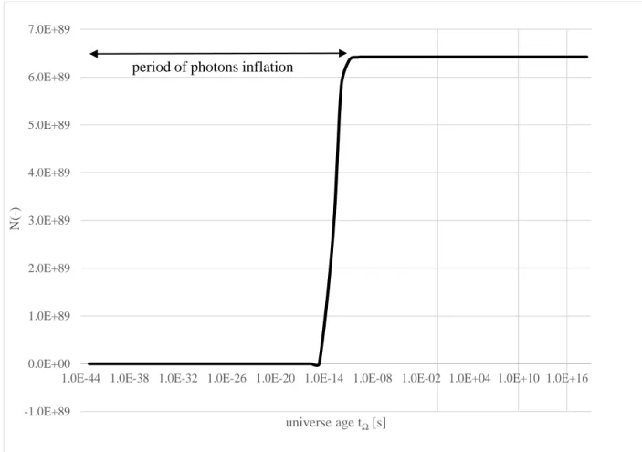
N(∞) = 64ζ(3)𝜋2 3 ( 𝑘𝑏𝑇Ω𝑡Ω ℎ ) 3 ~ 6,42 x1089 (constant)

The time period when the number of photons increases geometrically is called the photon epoch

(Figs. 1 & 2). The process leading to photon inflation is unknown but at every time increment, the

14

because photon energy remains slightly below Planck energy, Ep, (1.76x109 [J]) until time ~10-9

[𝑠] (Fig 3).

Figure 1: Inflation of photons number from 1 tp to 1x10-6 [s]

1.0E+00 1.0E+04 1.0E+08 1.0E+12 1.0E+16 1.0E+20 1.0E+24 1.0E+28 1.0E+32 1.0E+36 1.0E+40 1.0E+44 1.0E+48 1.0E+52 1.0E+56 1.0E+60 1.0E+64 1.0E+68 1.0E+72 1.0E+76 1.0E+80 1.0E+84 1.0E+88 1.0E+92

5.4E-45 5.4E-41 5.4E-37 5.4E-33 5.4E-29 5.4E-25 5.4E-21 5.4E-17 5.4E-13 5.4E-09

N( -) universe age t_Ω[s] 1 t_p(8g 10-9_{[s] ~10}34_t p~ 6,4x1089 0 t_p(1g

15

Figure 2: Number of Photons from 1 tp to 76,1 [𝐺𝑦]

Energy gain

Energy at the beginning of the universe is expressed as the energy of a single photon, the value of which is slightly lower than Planck energy, Ep. For N=1:

𝑈(0)= 0,9NkbTp = 0,9kbTp = 0,9Ep = 0,9c2 √ 𝑐 ℎ

2𝜋𝐺 = 1,76 x 10 9 _[J]

From a macroscopic standpoint, we assume that the universe does not undergo energy transfers

with other universes. Also, conventional energy is preserved in relation to time.

Photon gas energy in relation to time can be expressed in several equivalent ways for N >> 1:

U(t) = 3 PV = 4𝜎 𝑐 T 4_{V =3} 𝜁(4) 𝜁(3) N kb T ~ 2,7 N kb T -1.0E+89 0.0E+00 1.0E+89 2.0E+89 3.0E+89 4.0E+89 5.0E+89 6.0E+89 7.0E+89

1.0E-44 1.0E-38 1.0E-32 1.0E-26 1.0E-20 1.0E-14 1.0E-08 1.0E-02 1.0E+04 1.0E+10 1.0E+16

N(

-)

universe age t_Ω[s]

16 With the expression for N(t) obtained earlier:

U(t) = 2,7 N kb T = 64(4)( 𝑐𝑡+𝑟𝛼

ℎ𝑐 ) 3_(𝑘

𝑏𝑇)4 It can be written as:

U(t) =(64 ζ(4) 𝜋2𝑘𝑏4 ℎ3_𝑐3 ) ( (𝑐𝑡+𝑙𝑝)3 (−𝑡+𝑏)4) (𝑡Ω𝑇Ω)4 = 𝑈0( (𝑐𝑡+𝑙𝑝)3 (−𝑡+𝑏)4) (𝑡Ω𝑇Ω)4 Or still as: U(n) =(64 ζ(4) 𝜋2 ℎ3_𝑡 𝑝 ) ( (𝑛+1)3 (𝑛+𝑘′₎4) (𝑘𝑏𝑡Ω𝑇Ω)4

Where n is the whole number of Planck time units, tp, and k’ is a constant of universe (CMB

temperature is considered constant, as well as the age of the universe, 76,1 [Gy]), therefore:

n = t/tp 𝑘′ = (𝑡Ω 𝑡𝑝) ( 𝑇Ω 𝑇𝑝) = 3,57x 10 11 _𝑡 Ω = 8,57x1029 [𝑠] = 2,7x1013 [𝐺𝑦] For n=0, (N=1), we get: U(0) = 0,9kbTp = ( 64 ζ(4) 𝜋2 3 ℎ3_𝑡 𝑝 ) ( (1)3 (𝑘′₎4) (𝑘𝑏𝑡Ω𝑇Ω) 4 _{= (}64 ζ(4) 𝜋2𝑘𝑏4𝑡𝑝4 3 ℎ3 ) 𝑇𝑝 4 _{= 0,9E} p For t=𝑡_Ω, (N>>1) we get: U(tΩ)= (64 ζ(4) 𝜋 2_𝑘 𝑏4𝑡𝑝4 𝑘′4 ℎ3 ) 𝑇𝑝4 𝑡Ω =( 64 ζ(4) 𝜋2𝑘_𝑏4𝑇Ω4 ℎ3 ) 𝑡Ω 3

Maximum energy is reached for 𝑈̇(𝑡𝑚𝑎𝑥) = 0, or: 3𝑇 ℎ + 4 𝑇̇ ( 𝑡 ℎ+ 𝑙𝑝 ℎ𝑐) = 0 We get: 𝑡_𝑚𝑎𝑥=3 𝑡_𝑠 - 4𝑡_𝑝 = 3 𝑡Ω𝑇𝛺 𝑇𝑝 - 4𝑡𝑝 = 1,93x10 -32_𝑡 Ω - 4𝑡𝑝 For tΩ=76.1 [Gy], we get:

𝑡_𝑚𝑎𝑥= 1,38x10-13 [𝑠] = 2,57x1030 _t p

17 And for (tΩ=76,1 [Gy]):

𝑈_𝑚𝑎𝑥(𝑡_𝑚𝑎𝑥)= 3,57x1098 _[J]

Mass has not yet been created at this time because the temperature is in the order of 3,5x1031 _[K].

To get an idea of the sheer magnitude of energy, assuming that the entire mass created is in the

order of 1052 [kg], with relativistic energy-mass equivalence (=0,9), this corresponds to 2x1069

[J]; still an infinitissimal fraction of the energy in the universe.

Figure 4 below shows a graph for U(t) at tΩ=76,1 [Gy] (2,39x1018 [s]).

Figure 3:Photon mean energy from 1 tp to 1,4 [s]

Series1 1.0E+00 2.0E+08 4.0E+08 6.0E+08 8.0E+08 1.0E+09 1.2E+09 1.4E+09 1.6E+09 1.8E+09 en er g y [ J] universe age 𝑡Ω[s]

18

Figure 4: Universe total energy from 1 tp to 76,1 [Gy]

The energy gain, by a factor of 1089, can be explained by the increase in the number of photons,

also by a factor of 1089, during time period named photon inflation period, or 1.38x10-13 [s]. During

that photon inflation period, the number of photons increases, but the energy of each photon

remains approximately the same as the Planck energy, Ep (Fig 3). Moreover, during that timespan,

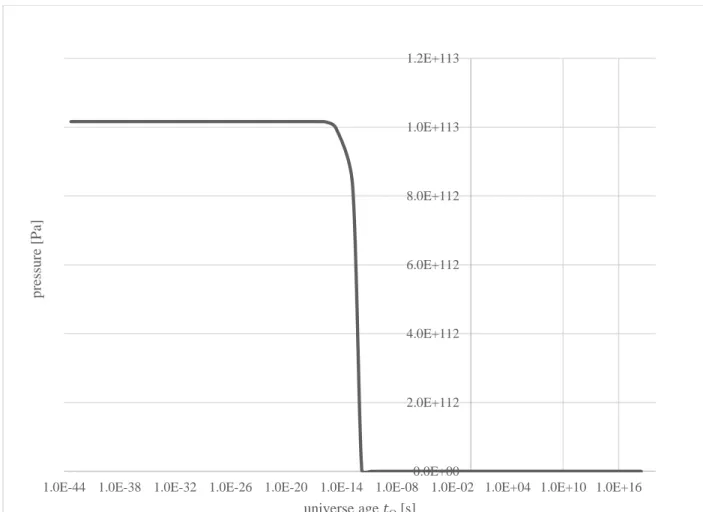
the temperature, as well as the pressure, remain practically stable at Tp and ~0.2Pp (Figs. 5 & 6).

Over that time, volume increases by a factor of 1086. Photons are created and this remains

unexplained, but this is due to the expansion of the universe volume, V and the availability of an

unknown energy. Such colossal energy comes from an existing potential which enchances the

1.0E+00 5.0E+97 1.0E+98 1.5E+98 2.0E+98 2.5E+98 3.0E+98 3.5E+98 4.0E+98 en erg y [ J] universe age 𝑡Ω[s] maximum energy at t_max= 3t_ΩT_/T_p- 4 t_p= 1,38x10-13_[s]

19

proliferation of photons, since nothing other than the above equations can predict energy levels.

The number of photons increases in a geometrical progression of nearly n3_{, where n is the number}

of Planck time units, tp.

Figure 5:Temperature from 1 tp to 76,1 [𝐺𝑦]

1.0E+00 2.0E+31 4.0E+31 6.0E+31 8.0E+31 1.0E+32 1.2E+32 1.4E+32

1.0E-44 1.0E-34 1.0E-24 1.0E-14 1.0E-04 1.0E+06 1.0E+16

tem p er atu re [K] universe age 𝑡_Ω[s]

20

Figure 6: Pressure from 1 tp to 76,1 [𝐺𝑦] A possible solution to the horizon problem?

We have seen that the number of photons increases in geometric progression of ~n3, where n is the

number of Planck time units, tp. Let us find an expression for the volume of the universe in relation

to the number of Planck time units, n, the boundary is moving at the speed of light:

𝑉(𝑛𝑡𝑝) = 4𝜋

3 (𝑐(𝑛 + 1)𝑡𝑝) 3

During the photon inflation period, the volume occupied by photons in relation to their number, N,

the Wien’s law, and the number of Planck time units can be estimated as:

𝑉_𝛾(𝑛𝑡_𝑝)~𝑁4𝜋 3 (𝜆) 3 = 𝑁4𝜋 3 ( 𝜎𝑤 𝑇) 3

With the equation found for temperature T:

0.0E+00 2.0E+112 4.0E+112 6.0E+112 8.0E+112 1.0E+113 1.2E+113

1.0E-44 1.0E-38 1.0E-32 1.0E-26 1.0E-20 1.0E-14 1.0E-08 1.0E-02 1.0E+04 1.0E+10 1.0E+16

p ress u re [P a] universe age 𝑡_Ω[s]

21 𝑉𝛾(𝑛𝑡𝑝) =𝑁 4𝜋 3 ( 𝜎𝑤 𝑇) 3 =𝑁4𝜋 3 ( 𝜎𝑤 −𝑡Ω𝑇𝛺 −𝑛𝑡𝑝 − 𝑡Ω𝑇𝛺_𝑇𝑝 ) 3

Let us express the photon volume quotient to the volume of the universe relative to the number of

Planck time units, n, and the number of photons N.

𝑉_𝛾(𝑛𝑡_𝑝) 𝑉(𝑛𝑡𝑝) = 𝑁 ( 𝜎_𝑤 −𝑡Ω𝑇𝛺 −𝑛𝑡_𝑝 − 𝑡Ω_𝑇𝑇𝛺 𝑝 ) 3 𝑐3_{(𝑛 + 1)}3_𝑡 𝑝3 After manipulation, the expression can be written as:

𝑉_𝛾(𝑛𝑡_𝑝) 𝑉(𝑛𝑡𝑝) = ( 𝑁 (𝑛 + 1)3) ( 𝜎_𝑤 𝑐𝑡𝑝𝑡Ω𝑇Ω𝑇𝑝 ) 3 (𝑛𝑡𝑝𝑇𝑝− 𝑡Ω𝑇Ω) 3

In the above expression, the only variables that evolve are the number of Planck time units, n, and

number of photons, N. The value of the quotient found for the entire age of the universe is:

𝑉𝛾(𝑛𝑡𝑝)

𝑉(𝑛𝑡𝑝) ~2,06 (constant)

What does this result mean? We have found that the volume occupied by photons, which increases

in geometric progression, is always slightly higher than the volume of the universe, and its

boundary is moving at the speed of light. Obviously, the value 2 is not accurate because the photons

are contained within the volume of the universe. The important value here is the constant. Now,

we can imagine the process occurring at every unit of Planck time. The number of photons

potentially increases around the volume created (at the boundary?) at every unit of Planck time;

22

Moreover, at every unit of Planck time, the already existing photons also undergo 𝛾𝛾 exchange. This 𝛾𝛾 exchange process is made possible by the quotient between the number of new photons around the boundary of the existing photons at Planck time, prior to the progression from the

maximum 8 to the minimum 1, or 8 at the first unit of Planck time, down to 1 when the number of

photons no longer increases, or:

𝑁((𝑛+1)𝑡𝑝) 𝑁(𝑛𝑡𝑝) ~ 8 1 (𝑛 = 0) → 1089 1089(𝑛 > 1034(10−9[s]))=1

This is a very important result, the 𝛾𝛾 exchange are made possible when the number of photons increases further (ratio →1). This occurs around 10-9 [𝑠] after the beginning. Therefore, after that time, the 𝛾𝛾 exchange remain causal. Moreover, during the photon inflation period, when the 𝛾𝛾 exchange are not entirely causal, we note that the temperature is steady at Planck temperature (Fig. 6). Hence, even during the photon inflation period, the information exchange between

photons cannot be entirely causal, that information is not necessary from a thermodynamic

23

Figure 7:Number of photons and temperature function of cosmic time from 10-24_{[s] to 10}-9_[s]

This mechanism makes it possible to solve the horizon problem for the photon inflation period, or

energy creation period, if the high-energy 𝛾𝛾 exchange principle is accepted. Photon-photon exchange are a fact that has been confirmed at CERN (Kłusek-Gawenda, Lebiedowicz and

Szczurek, 2016). Photon exchange energy, ggfor that experiment was an estimated ~15-20 [GeV],

while the energy of photons at the beginning was ~0.9 Ep, or ~1019 _{[GeV]. Of course, this goes}

beyond the purpose of this paper since 𝛾𝛾 exchange will require much more study. However, the process makes it possible to solve the event horizon problem, as the photon energy volume is

always in phase with that of the volume of the universe. In brief, these periods are:

0 < 𝑡 < ~10−16[s] (z~1033) (causality, T~constant) 1.0E+00 1.0E+04 1.0E+08 1.0E+12 1.0E+16 1.0E+20 1.0E+24 1.0E+28 1.0E+32 1.0E+36 1.0E+40 1.0E+44 1.0E+48 1.0E+52 1.0E+56 1.0E+60 1.0E+64 1.0E+68 1.0E+72 1.0E+76 1.0E+80 1.0E+84 1.0E+88 1.0E+92 1.0E+00 1.0E+02 1.0E+04 1.0E+06 1.0E+08 1.0E+10 1.0E+12 1.0E+14 1.0E+16 1.0E+18 1.0E+20 1.0E+22 1.0E+24 1.0E+26 1.0E+28 1.0E+30 1.0E+32 N [-] universe age t_Ω[s]

period of partial causality lost (approxi. 106g)

T

[K

24

~10−16[s] < 𝑡 < ~10−9[s] (z~1026) (partial causality) ~10−9_{[s] (z~10}26_{) < 𝑡 (causality, N~constant)}

The CMB is at z~1100, or well after the start of the causality recovery period. We will see that the

last scattering surface of the model is ~69 [My] after the beginning. This leaves ~1058 Planck time

units to restore causality. It can be reasonably assumed that at recombination time the universe had

enough time to recover all of the causality, and that is why we can observe isotropy in the CMB

(McCoy, 2014).

Early baryogenesis (protons, neutrons) and leptons (electrons, neutrinos)

Interactions between photons and matter are complex and beyond the scope of this paper.

Moreover, relativistic effects have to be considered as particle speeds approach the speed of light

upon creation. In this paper, we describe a creation mechanism for the main particles (p, n, e and

) to demonstrate the coherence of the model. During early baryogenesis, at very high temperature (mc2<<kT), the Maxwell-Juttner M-J (relativist) statistical law is used to predict particle properties

(fermions and letpons). Moreover, the presence of antiparticles must be considered, along with the

creation-annihilation process. In this paper, we want to estimate the total barionic mass produced

at the end of baryogenesis. We are able to estimate the full potential of mass creation in the universe

using the mass-energy equivalence, since we are estimating total energy. The following expression

is used to find the mass creation potential. Note that here, we assume that the energy in the universe

is conventional: 𝑀_𝑝𝑜𝑡= √1−𝛽2 𝑈(𝑡Ω) 𝑐2 = ( √1−𝛽2_{64 ζ(4) 𝜋}2_𝑘 𝑏4𝑇Ω4 𝑐2 _ℎ3 ) 𝑡Ω3

We can see that the mass creation potential is relative to the cube of the age of the universe. For

25

produced is 4,81x1048 [kg], which is ~104 smaller than the approximate estimated mass of the

universe (1052 à 53 _{[kg]) (Carvalho, 1995). This clearly shows that to maintain this estimated mass,}

the existence of a source of non-conventional energy, or dark energy, has to be considered. Another

possibility is to extend the age of the universe. Evidently, the precise mass of the universe is

unknown. Supposing an estimated mass variation factor of 102 and conventional energy, we have

to assume, based on the above equation, that the universe is much older than 13,8 [Gy] (visible

universe ~ 13,8 [Gy]). Typically, for a mass potential in the order of 1050 _{to 10}53 _{[kg], the age of}

the universe must be somewhere between 37,9 [Gy] and 379 [Gy]. To estimate the volumic

quantity of protons and neutrons created, the Maxwell-Juttner statistical distribution is used, as

follows (Cercignani and Medeiros Kremer, 2002):

𝑛𝑝,𝑛 = 4𝜋𝑐𝑚𝑝,𝑛2 𝑘𝑏𝑇𝐾2(𝜇) ℎ3 𝑒 −𝑚𝑝,𝑛 𝑐2 𝑘𝑏𝑇√1−𝛽2 With: 𝜇 = 𝑚𝑝,𝑛𝑐2 √1−𝛽2_𝑘 𝑏𝑇

and 𝐾₂(𝜇) the modified Bessel function of the second kind. In this distribution, the stop temperature for the definitive creation of protons and neutrons must be

specified, as well as the relativistic speed of created fermions. The value of 𝛽 poses a problem, in fact, a lower value allows to create more mass and conversely also. We will see further from the

energetic form of the Friedmann equation that an average value of 𝛽 can be estimated at 𝛽~0,866. However, the global energy equation imposes a maximum value for beta to 𝛽~0,998 _{in order to} maintain the positive energy balance at the scale of the universe (for the entire cosmic time):

∆𝑈 = 𝑈𝛾− 𝑈𝑀 = 2,7 𝑁𝑘𝑏𝑇 −

𝑀_𝑡𝑜𝑡𝑐2 √1 − 𝛽2 > 0

26 𝑇̅𝑝𝑟,𝑛𝑒= 𝑚𝑝𝑟,𝑛𝑒𝑐2 √1−𝛽2 𝑘𝑏 = 𝐶1 (−𝑡𝑝𝑟,𝑛𝑒+𝑏)

This mean photon energy appears at proton and neutron temperature and time, or tpr,ne , after the

beginning of expansion: Therefore: tpr,ne = b - 𝑘𝑏𝐶1 𝑚𝑝,𝑛𝑐2 √1−𝛽2 = 𝑡Ω𝑇Ω 𝑇𝑝 + 𝑘𝑏𝑇Ω𝑡Ω 𝑚𝑝,𝑛𝑐2 √1−𝛽2 = [𝑇Ω 𝑇𝑝 + 𝑘𝑏𝑇Ω 𝑚𝑝,𝑛𝑐2 √1−𝛽2 ] 𝑡Ω

For 𝑡Ω=76,1 [Gy] = 2,39x1018[s] and =0,9986, we find:

tpr ~ 31345 [𝑠] ~ 0,3627 [𝑑] after the beginning of expansion 𝑇̅_𝑝𝑟=2,08x1014 [𝐾]

tne ~ 31303 [𝑠] ~ 0,3623 [𝑑] after the beginning of expansion 𝑇̅𝑛𝑒= 2,09x1014 [𝐾]

The creation potential (without annihilation, 𝑝𝑝 ̅ , or disintegration, 𝑛) for protons and neutrons at this time is:

𝑛𝑝 = 𝑉4𝜋𝑐𝑚𝑝2𝑘𝑏𝑇𝑝𝑟𝐾2(𝜇) 𝑒 ℎ3 = 16𝜋2𝑐4𝑡𝑝𝑟3 𝑚𝑝2𝑘𝑏𝑇𝑝𝑟𝐾2(𝜇) 3 𝑒 ℎ3 = 2,1700 x10 86 and neutrons: 𝑛_𝑛 = 𝑉4𝜋𝑐𝑚𝑛 2_𝑘 𝑏𝑇𝑛𝑒𝐾2(𝜇) 𝑒 ℎ3 = 2,1689x10 86 Where = 𝑚𝑐 2 √1−𝛽2_𝑘 𝑏𝑇

The creation of neutrons occurs 43 [𝑠] prior to proton fixation, allowing to capture p+n before complete disintegration of the neutrons (881 [s]). To estimate the final number of protons and

27

we assume that baryonic asymmetry prevails according to a normally accepted proportion of one

stable baryon created for every 109 𝑝𝑝̅ and 𝑛𝑛̅ annihilations (Dolgov, 1998). Moreover, neutrons are captured and disintegrate in an accepted proportion of one neutron captured for every four

neutrons disintegrated (the calculated ratio is 0,188 for 43 [𝑠] of disintegration time). Then, in a universe aged 76,1 [Gy], we estimate the stable masses to be:

Mp ~ 10−9(𝑛𝑝𝑚𝑝+ 0,8𝑛𝑛𝑚𝑛)~ 6,53x1050 [𝑘𝑔] Mn ~ 0,2 𝑥 10−9𝑛𝑛𝑚𝑛~ 7,25x1049 [𝑘𝑔]

However, with the exponential disintegration of neutrons, ~95 % of them will still be available for

capture (formation of deuterium at ) after 43 [𝑠] before the creation of protons.

Also, an equation can be found for the baryon-photon ratio, 𝜂𝐵. Initially assuming that the baryon-photon ratio can be expressed as the proton and neutron creation potential after annihilation and

disintegration, expressed in a number of protons (at ) only, after manipulation, we get the

following equation and a maximum value for the ratio:

𝜂_𝐵 = 𝑛𝑏(𝑡𝑝𝑟) 𝑛𝛾(𝑡𝑝𝑟)~ 2𝑛𝑝(𝑡𝑝𝑟) 𝑁(𝑡𝑝𝑟) =10 −9 2𝑉4𝜋𝑐𝑚𝑝2 𝑘𝑏𝑇𝑝𝑟𝐾2(𝜇) 𝑒 ℎ3 64 ζ(3)𝜋2₃ (𝑘𝑏𝑇𝑝𝑟𝑡𝑝𝑟_ℎ ) 3 =10−9 (1−𝛽2)𝐾2(𝜇) 2𝑒ζ(3) =10 −9(1−𝛽2)𝐾2(𝜇) 6,53

The above constant ratio solely depends on 𝛽 associated with protons during (relativistic) creation, and the modified Bessel function of the second kind, 𝐾2(𝜇) (Maxwell-Juttner distribution), as well as the numbers,

e,

𝜂𝐵 = 10−9 (1−𝛽2)𝐾2(𝜇) 6,53 = 10 −91,62 6,53 = 2,48x10 -10

28

The resulting value of 2,48x10-10 is lower than the results of the estimates yielded by the ΛCDM

model (Kirilova and Panayotova, 2015), based on Planck measurements. Indeed, the estimated

quotient is not a direct measurement, but rather an estimate that is partly based on ΛCDM model

assumptions and observations, or:

𝜂_𝐵 = 𝑛𝑏

𝑛𝛾 = 6,108 ± 0,038 x10 -10

However, a small change in the oft-stated ~10-9 _{particle-antiparticle annihilation factor and 𝛽 can} proportionally change the result.

Electrons

The Maxwell-Juttner statistical distribution for electrons:

𝑛𝑒𝑙 = 4𝜋𝑐𝑚𝑒2𝑘𝑏𝑇𝐾2(𝜇) ℎ3 𝑒 −𝑚𝑒 𝑐2 𝑘𝑏𝑇√1−𝛽2 With: 𝜇 = 𝑚𝑒𝑐2 √1−𝛽2_𝑘 𝑏𝑇

This mean energy of photons occurs at stop temperature and electron time, expressed as tel, after

the beginning of expansion (=0,9986):

𝑇̅_𝑒𝑙= 𝐶1 (−𝑡𝑒𝑙+𝑏) = 𝑚𝑒𝑐2 √1−𝛽2 𝑘𝑏 = 1,13x10 11 _[𝐾] Therefore: tel = b - 𝑘𝑏𝐶1 𝑚𝑒𝑐2 √1−𝛽2 = 𝑡Ω𝑇Ω 𝑇𝑝 + 𝑘𝑏𝑇Ω𝑡Ω 𝑚𝑒𝑐2 √1−𝛽2 = [𝑇Ω 𝑇𝑝+ 𝑘𝑏𝑇Ω 𝑚𝑒𝑐2 √1−𝛽2 ] 𝑡Ω

For 𝑡_Ω=76,1 [Gy] = 2,39x1018[s] and =0,9986, we get:

29

The electron creation potential (without 𝑒𝑒̅ annihilation) at this time is: 𝑛_𝑒 = 𝑉4𝜋𝑐𝑚𝑒 2_𝑘 𝑏𝑇𝑒𝐾2(𝜇) 𝑒 ℎ3 = 16𝜋2𝑐4𝑡𝑒𝑙3𝑚𝑒2𝑘𝑏𝑇𝑒𝐾2(𝜇) 3 𝑒 ℎ3 = 2,1700x10 86

To estimate the final number of electrons, the respective antiparticle creation and annihilation must

be considered. To do so, let us assume that lepton asymmetry prevails according to a proportion

of one stable electron created for every 109 𝑒𝑒̅ annihilations. For 𝑡Ω=76,1 [Gy]:

Me = 10−9(𝑛_𝑒𝑚_𝑒+ 0,8𝑛_𝑛𝑚_𝑒)~ 3,55x1047 [𝑘𝑔]

Finally, the following total mass for the creation of electrons, protons and neutrons is achieved:

Mt = Mp + Mn+ Me = 7,26x1050 [𝑘𝑔]

The ratio of positive (p) to negative (e) charges is strictly equal to one, since the beta disintegration

of a neutron produces one proton and one electron. Therefore, the Maxwell-Juttner relativistic

distribution predicts an electrically neutral universe in terms of protons, neutrons and electrons.

Based on this relativistic distribution and for a specific cosmological model, the following dynamic

temperature-time relation must be met during the proton-electron production process. Indeed, the

exact mass ratio is known:

𝑚𝑝(𝑡) 𝑚𝑒(𝑡) = [ 𝑡_𝑒𝑙3𝑇𝑒𝑙 𝑡𝑝𝑟3 𝑇𝑝𝑟] 1 2 ⁄ = 1836,15

Using the above model and equations, along with the Maxwell-Juttner distribution, the dynamic

evolution of the model’s variables yields a very realistic ratio: 𝑚_𝑝(∞)

30

Cosmic neutrinos from SN1987A

Cosmic neutrino mass can be estimated using the above relation. Indeed, cosmic neutrino mass

can be expressed according to proton or electron mass, as:

𝑚𝜈(𝑡) 𝑚𝑒(𝑡) = [ 𝑡_𝑒𝑙3𝑇𝑒𝑙 𝑡𝜈3𝑇𝜈] 1 2 ⁄

The above equation can be developed with the electron temperature equation along with electron

creation time. After some manipulations, we get the following expression for cosmic neutrino

mass: 𝑚_𝜈~ (𝑘𝑏√1−𝛽2𝑚𝑒𝑙2𝑇𝑒𝑙𝑇𝑝 𝑐2_𝑇 Ω ) 1/3 𝑡𝑒𝑙 𝑡Ω

The only undetermined variable in the above equation is the mean of cosmic neutrinos during

their creation. The use of is not an easy choice since this particle is still relatively unknown and

has three known states (oscillations). Using 𝛽𝑆𝑁1987𝐴 , estimated from Stodolsky’s observations of SN1987A in (Stodolsky, 1988), (≤0,999999998), the maximum neutrino mass can be

expressed as:

𝑚𝜈𝑆𝑁1987𝐴 ≤ 8,69x10-32 [𝑘𝑔] = 48,7 [keV𝑐−2]

While this is too high a mass for electron neutrinos (<2,5 [eV𝑐−2]), it fits well for muon neutrinos (≤ 170 [keV𝑐−2_]).

In addition, this found value is within the estimated limit of Benes et al, (2005) for the sterile

neutrino mass of SN1987A (10-100 [keV𝑐−2_{]). Also, Bezrukov (2018), from a detailed analysis} of the possibilities for the mass of the sterile neutrino, find a value ~ 3,3 [keV𝑐−2]that it identifies as a possibility that dark matter is made of sterile neutrinos. However, we will see that the amount

of neutrino generated cannot explain the abundance of dark matter predicted by the ΛCDM model

31

This maximum mass is situated between that of the electron neutrino and muon neutrino, or:

𝑚𝜈𝑒 < 𝑚𝜈

𝑆𝑁1987𝐴 _{< 𝑚} 𝜈𝜇

2,5𝑥10−3_[keV𝑐−2_{] < 48,7 [keV𝑐}−2_{] < 170[keV𝑐}−2_]

The resulting mass for cosmic neutrinos is ~ 10 times lower than that of electrons, and their speed

is practically the speed of light c. Of course, cosmic neutrinos can be found to have different

masses depending on the assumptions made for  The goal here is not to derive precise neutrino

mass, which is beyond the scope of this paper. Using the neutrino mass obtained above, the time,

temperature, quantity, and total mass of cosmic neutrinos can be achieved using the

Maxwell-Juttner distribution: 𝑇̅𝜈= 𝐶1 (−𝑡𝜈+𝑏) = 𝑚𝜈𝑐2 √1−𝛽2 𝑘𝑏 = 8,9x10 12 _[K] Therefore: t = b - _{𝑚𝜈𝑐2}𝑘𝑏𝐶1 √1−𝛽2 = 𝑡Ω𝑇Ω 𝑇𝑝 + 𝑘𝑏𝑇Ω𝑡Ω 𝑚𝜈𝑐2 √1−𝛽2 = [𝑇Ω 𝑇𝑝 + 𝑘𝑏𝑇Ω 𝑚𝜈𝑐2 √1−𝛽2 ] 𝑡_Ω

For 𝑡_Ω=76,1 [Gy] = 2,39x1018[s] and =0,999999998, we get:

t ~ 7,315x105 [𝑠] ~ 8,4 [𝑑] after the beginning The neutrino creation potential (without 𝑣𝜈̅ annihilation) at this time is:

𝑛_𝜈 = 𝑉4𝜋𝑐𝑚𝜈 2_𝑘 𝑏𝑇𝜈𝐾2(𝜇) 𝑒 ℎ3 = 16𝜋2𝑐4𝑡𝜈3𝑚𝜈2𝑘𝑏𝑇𝜈𝐾2(𝜇) 3 𝑒 ℎ3 = 3,19x10 80

Maximum mass of neutrinos (without annihilation), after a few manipulations for 𝑡Ω=76,1 [Gy], is acheived by:

32

A conclusion can be made here, neutrino mass (without annihilation) represents a maximum

~4,2 % of proton mass. Based on the model, cosmic neutrino mass cannot explain the origin of the

missing mass. Furthermore, based on the Maxwell-Juttner distribution, cosmic neutrinos appeared

before electrons, but after baryons. Another way to proceed involves using the known neutrino

mass and look at the creation period and predicted mass, but we still get a predicted neutrino mass

that is much smaller than that of baryons.

Let us revisit the total predicted mass of ~7 x1050_{, which is relatively lower (17 to 350 times) than}

the oft-mentioned total mass of the universe (1,25x1052 to 2,5x1053). However, total mass is

relative to the age of the universe. Hence, baryon mass could be increased by increasing the age

of the universe or by reducing the particle-antiparticle annihilation factor. However, we will see

that the so-called missing mass is not that essential to explain galaxy rotation. The mass can be

increased, but we will see that the data from the Planck probe give us the mass vs. energy ratio,

which allows us to calculate an approximate age of the universe that partly meets the proportions.

We will come back to this argument later. With the energy-mass equivalence, when the ratio of

total created mass energy to total universe energy at the time of electron production (around the

end of the main leptogenesis) is obtained, we get =0.001, or a low non-relativistic speed of the

baryonic mass, but still within the range of velocity for the MW:

𝐸𝑚𝑎𝑠𝑠 𝐸𝑡𝑜𝑡𝑎𝑙 = 𝑀𝑡𝑐2 √1−𝛽2 𝑈(𝑡𝑒𝑙) = 6,43𝑥1067 2,72𝑥1078 = 2,3x10 -11

This energy ratio confirms that the universe, during early leptogenesis, or at the end of the creation

of the particles that make up most of the mass, was vastly influenced by radiation (radiation

universe) and that the effects associated with mass, such as gravity, were negligible compared to

33

Mean total energy of the universe 13,8 [Gy] after the beginning is:

𝑈_{𝑡𝑜𝑡𝑎𝑙} ~ 2,05 x1069 [J]

That energy, when converted to energy-mass equivalence, yields the following mass (=0,001):

𝑀_{𝑒𝑞𝑢𝑖−𝑒𝑛𝑒𝑟𝑔𝑦}= 2,0𝑥10

69_√1−𝛽2

𝑐2 = 2,23x10

52 _[kg]

The ratio between the baryonic mass and potential energy-mass for the time period ~1 to 13,8 [Gy],

which can be observed by instruments like the Planck probe, would be:

[ 𝑀𝑡

𝑀𝑒𝑞𝑢𝑖−𝑒𝑛𝑒𝑟𝑔𝑦]_{𝑜𝑏𝑠𝑒𝑟𝑣𝑎𝑏𝑙𝑒}=

7,26x1050 _kg

2,23x1052 _kg ~ 0,032

That energy-matter ratio is smaller than the estimate made from Planck measurements, an

estimated ~0,31 (regular and dark matter). Howerver, that ratio was calculated using the CDM

model, which includes dark matter and dark energy as parameters. If dark energy is removed from

the equation and only the CDM-estimated baryonic mass is considered, the result is closer, or

0,048.

Let us calculate the mean volumic mass of the universe at the end of proton production:

𝜌_𝑝𝑟𝑀𝑝𝑟 𝑉  7,26x1050 _kg 4𝜋 3𝑟 3  7,26x1050_kg 4𝜋 3(9,39𝑥10 12₎32x10 11 _{[kg 𝑚}−3_]

Such density is much lower than the approximate density of a proton (~6,7x1017 _{[kg 𝑚}−3_]), showing that the universe could have contained that amount of mass at that time.

We have not yet considered the electrostatic energy associated with protons and electrons. Let us

assume that the Coulomb charge was attributed to protons and electrons at the time of baryogenesis

and leptogenesis. Indeed, the electrostatic energy of protons and electrons contained in the sphere

34 𝐸_𝑝𝑟𝑒𝑙 ₌ 3 5 𝑘𝑒 (𝑛𝑝𝑟𝑞𝑝𝑟)2 𝑟𝑝𝑟 = 3 5 8,987𝑥10 9 (3,9𝑥1077 𝑥 1,6021𝑥10−19)2 9,39𝑥1012 = 2,24x10 114 _[J] 𝐸_𝑒𝑙𝑒𝑙 = 3 5 𝑘𝑒 (𝑛𝑒𝑙𝑞𝑒𝑙)2 𝑟𝑒𝑙 = 3 5 8,987𝑥10 9 (3,9𝑥1077 𝑥 1,6021𝑥10−19)2 1,72𝑥1016 = 1,22x10 111 _[J]

However, because the quantity of protons, npr, and electrons, nel, created is identical, we get

(including neutron disintegration):

npr = nel = 3,9x1077

Therefore, the total charge becomes neutral, and the potential energy disappears in the aftermath

of electron production. However, the electrostatic potential remains active for ~666 days, which

corresponds to the time difference from the appearance of protons and electrons. We will see that

the time difference or delay is the cause of a major so-called baryon-free (empty) zone, except for

cosmic neutrinos and others neutral particules.

Thus, the actual baryon-photon ratio for the entire universe (𝛽~0,001) can be estimated: B 𝑛𝐵 𝑛𝛾 𝑛𝑝𝑟+𝑛𝑛 6,42x1089 4,33𝑥1077 6,42x1089~6,7x10 -13

A constant value for the age of the universe after baryogenesis, assuming conventional proton and

electron half-lives.

This baryon-photon ratio is ~1000 times smaller that the Bernreuther estimate (2002). This is due

to the calculated baryon mass, which is 500 to 1000 times smaller, ~1050 [kg], than the

35

Temperature variations in the CMB

A possible way to address partially the temperature variations in the CMB is found in variations

in the energy of the universe during baryogenesis and leptogenesis. Indeed, when protons,

neutrons, and electrons were created, a considerable amount of energy was drawn from the photons

for the creation of the particles. That one-time energy shift in the early expansion of the universe

(0,362 day for the protons and 666 days for the electrons) surely caused a disruption in the photon

gas. Moreover, the creation of matter was likely uniform in the volume, but the energy demand

may have caused a local disruption over time for the neutrons, and later for the protons and

electrons. Let us calculate that energy disruption for the baryons during baryogenesis, relative to

the energy of the universe in the pre-baryon era, and for the electrons, relative to the energy of the

universe at that time, or (𝛽 𝑜𝑓 𝑝𝑟𝑜𝑡𝑜𝑛𝑠, 𝑒𝑙𝑒𝑐𝑡𝑟𝑜𝑛𝑠 = 0,986 𝑎𝑛𝑑 𝛽 𝑛𝑒𝑢𝑡𝑟𝑖𝑛𝑜𝑠 = 0,999999998) : ∆𝑬𝒃𝒂𝒓𝒚𝒐𝒏 𝑬 = ∆𝐸_𝑀𝑡 𝐸𝑡𝑜𝑡𝑎𝑙 = (𝑀𝑝+𝑀𝑛)𝑐2 √1−𝛽2_𝑈(𝑡 𝑝𝑟) = 1,25𝑥1069𝐽 9.05𝑥1081_𝐽 = 1,38x10 -13 ∆𝑬𝒆𝒍𝒆𝒄𝒕𝒓𝒐𝒏 𝑬 = ∆𝐸_𝑀𝑡 𝐸𝑡𝑜𝑡𝑎𝑙 = 𝑀𝑒𝑐2 √1−𝛽2_𝑈(𝑡 𝑒𝑙) = 6,12𝑥1065𝐽 7,81𝑥1078_𝐽 = 9,15x10 -14 ∆𝑬𝒏𝒆𝒖𝒕𝒓𝒊𝒏𝒐 𝑬 = ∆𝐸_𝑀𝑡 𝐸𝑡𝑜𝑡𝑎𝑙 = 𝑀𝜈𝑐2 √1−𝛽2_𝑈(𝑡 𝜈) = 3,94𝑥1070𝐽 5,0𝑥1080_𝐽 = 5,88x10 -11

When that energy is put in relation with that of the blackbody, the energy ratio can be expressed

in terms of temperature as:

∆𝑻𝒃𝒂𝒓𝒚𝒐𝒏 𝑻 = [ ∆𝑬𝒃𝒂𝒓𝒚𝒐𝒏 𝑬 ] 𝟏/𝟒 = (1,38x10-13)1/4 ~ 6,1x10-4 ∆𝑻𝒆𝒍𝒆𝒄𝒕𝒓𝒐𝒏 𝑻 = [ ∆𝑬𝒆𝒍𝒆𝒄𝒕𝒓𝒐𝒏 𝑬 ] 𝟏/𝟒 = (9,15x10-14)1/4 ~ 5,5x10-4

36 ∆𝑻𝒏𝒆𝒖𝒕𝒓𝒊𝒏𝒐 𝑻 = [ ∆𝑬𝒏𝒆𝒖𝒕𝒓𝒊𝒏𝒐 𝑬 ] 𝟏/𝟒 = (5,88x10-11)1/4 ~ 3x10-3

Following measurements made by Planck, the analysis and explanation of temperature variations in the CMB became priorities. Ever since the initial analyses and Fixsen’s synthesis (Fixsen, 2009), assessments of temperature variations in the CMB continually varied as new interpretations were made and instruments were perfected. Variations sit within a range of values put forth by separate authors. Without going into finer detail, the range of values is as follows:

Planck, 2015 Fixsen, 2009 [±𝟐𝟕𝒎𝑲 𝟐,𝟕𝟐𝟐 𝑲] < [ ∆𝑻 𝑻]_𝑒𝑥𝑝< [ ±𝟓𝟕𝟎µ𝑲 𝟐,𝟕𝟐𝟓𝟒𝟖 𝑲] ±9,9x10-3_{< [}∆𝑻 𝑻]_𝑒𝑥𝑝< ±2,1x10 -4

This shows that baryogenesis and leptogenesis, or variation of energy for the creation of protons, electrons and neutrinos, is in the order of magnitude of the overall temperature variations in the CMB (energy disruption or negative energy jump of the photons during the creation of matter). Could those temperature variations in the CMB be partially caused by successive energy jumps during particle creation, in addition to the vibrational mode of baryons (Eisenstein, Zehavi, Hogg et al., 2005) ? Moreover, analyses of the variations do not seem to show any anisotropy, except for great empty zones. This supports the notion of isotropic energy variations for the entire volume that is compatible with the creation of a uniform mass in the volume. Finally, because protons, neutrons and electrons, and the particle fusion cycles, occurred at different times and different energy levels for the photons in the photon gas, notable variations (Δ𝑇/𝑇)_𝑖 could be found in the variations of energy spectrum of the CMB in line with the energy levels successively implicated

37

in beryogenesis and leptogenesis, and at successive times for the protons-neutrons, electrons, deuterium, etc.

Expanding 3d-sphere of matter

An order of magnitude for the avarage speed of baryonic matter can be calculated with a theoretical mean mass density of the universe, the Hubble-Lemaître expansion law, the cosmic time and the assumption that the boundary of the universe is moving constantly at the speed of light.

Let us suppose that this sphere of matter was at state 1 at the time of early creation of great structures like galaxies (<2 [Gy]), whose boundaries were expanding at the speed of light towards state 2, or the current age of the universe, written as tΩ. Let us also suppose a material point in the sphere in state 1 (e.g. the original bulbe of matter at the center of the MW), which undergoes expansion until today. That point is not located at the mathematical centre of the sphere, but at a given location written as r1 at state 1. The material point evolves towards a material position 2 in state 2, moving at a mean speed 𝛽 ̅ (non-relativist). Moreover, considering expansion and displacement at the mean speed in the direction of expansion, the following equation yields the position of the material point at state 1 at time t0 in the sphere of matter at the time of state 2 (universe age tΩ): 𝑡₀= 𝑡Ω 𝑡1 𝑟1 𝑐 + 𝑡1 𝑡Ω 𝛽̅(𝑡Ω− 𝑡1) = 𝑡Ω 𝑟1 𝑅1 + 𝑡1 𝑡Ω 𝛽̅(𝑡Ω− 𝑡1) Where: 𝑅1=𝑐𝑡1 ; 𝑅Ω = 𝑅2 = 𝑐𝑡Ω

The first term is the expansion of the material point in the expanding volume during the time period, and the second term is the effect of the speed modulated by the inverse of expansion. The equation has four mathematically independent variables that must be compatible from a physics standpoint.

38

Indeed, for each quartet (𝑟1, 𝑡1, 𝑡Ω, 𝛽̅), the value of 𝑡0 must be lower than or equal to 𝑡Ω, which limits possibilities, or still, forces a restriction on variable 𝛽̅. In this paper, we only consider the mean value of β̅ for a sphere of matter undergoing Hubble-Lemaître expansion, the boundary of which is moving at β=1. The cosmological principle states, at least, that there are no preferred positions. However, expansion of the universe occurs in a precise order of events, each appearing at its own cosmic time, which leads to the idea that for a much larger universe than what we can observe today, one can imagine relative positions within that chronological universe. Moving forward with that idea, one can estimate an approximate position for the MW in the sphere universe. Indeed, we will see in the next section, dealing with a mass rotation model for a few galaxies with the combined action of gravitational force and cosmological gravity, that initial formation of the MW could have started around 150-190 [My] after the beginning, and that main formation could have taken 380-450 [My]. Therefore, let us start with a sphere universe of state 1 at time 1 [Gy] (t1=1 [𝐺𝑦] ), that is a sphere of matter that is large enough to contain the MW bulbe. Initial formation of the bulbe yields 𝑟1

𝑅1

⁄ =0,15-0,19 [Gy]/[𝐺𝑦]. Moreover, by selecting 𝛽̅ according to an equation developed in the next section (𝛽̅~2𝑥10−3_{), and 𝑡}

0, the age of the universe calculated by Planck (13,8 [Gy]) at our observation position, we get an approximate range of ages for the universe today:

𝑡_Ω~ 73 to 92 [Gy]

That number must be seen as sufficient to create the required energy for the universe to generate a baryonic mass that is close to the mass estimated from observations of the cosmos, while providing a possible explanation for the formation periods and rotations of the galaxies being studied.

39

Pressure in the CMB and the Casimir effect: A possible age of the universe

The Casimir Effect is often used to explain what authors call vacuum energy or vacuum force. There is a model we can use to further analyze this effect and see if it can be partially explained and provide useful information.

Readers can refer to numerous works on the Casimir Effect and its electromagnetic origin (Kawka, 2010). If the Casimir force is expressed as shown in works where parallel plates are used, we get the following equation:

Fc = (𝜋 2

240) ℎ 𝑐 2𝜋𝑙4 S

Where 𝑙represents the distance between the parallel conductive plates, and S is the surface of the plates. The constant is obtained from the integration of potential photon vibration modes between the plates (the space between the plates act as a resonant cavity for the photons). This normally attractive force can be expressed as radiation pressure:

Fc =𝑃_𝑐 S

The quantities of energy in the universe on a per-era basis are known, which can be expressed in the form of mean density of energy in the volume, as:

Fc = (𝑈(𝑡) 𝑉(𝑡)) S

From the photon gas energy expression, an expression of Casimir force, from a standpoint of properties at time t, is written as:

Fc(t) = (𝑁 ℎ 𝜗 𝑉 ) S = ( 2𝜋 𝑁 ℎ 𝑐 2𝜋𝑉𝜆 ) S = ( 2𝜋 𝑁(𝑡) 𝑉(𝑡)𝜆(𝑡)) ℎ 2𝜋𝑐S

40

Where N is the constant number of photons after the photon inflation period, or about 10-13_[s] (N~6,4x1089_{). Moreover, if we postulate that Casimir pressure is generated by CMB photons at} our position t0, then:

Fc = Pc S = (2𝜋𝑁(∞) 𝑉0𝜆𝑐𝑚𝑏

) ℎ 2𝜋𝑐S

The above Casimir Effect equation makes it possible to calculate pressure at time t0 (at our position in the universe) when the mean wavelength of photons in the CMB is known. As with CMB temperature, Casimir pressure is an observable property of the universe. That wavelength is well known and derived from the Wien’s law, as:

cmb= 𝜎𝑤 𝑇𝑐𝑚𝑏 =

2,89777𝑥10−3

2,728 = 1.06x10 -3 _[𝑚]

In a manner of speaking, that pressure is the same as theoretical pressure in a vacuum (CMB radiation pressure), considering the fact the energy of the universe decreased when the particles were created. To determine that pressure, we could estimate the position of the observer, t1, in the universe. To do so, we know the expression for photon gas pressure at the same time, t1, and we get the following expression to determine a possible position in the universe or cosmic time:

Pc= Pgas g (2𝜋𝑁(∞) 𝑉1 𝜆𝑓𝑑𝑐1 ) ℎ 2𝜋𝑐 = 𝜁(4)𝑁(∞)𝑘𝑏𝑇1 𝜁(3)𝑉1 ( ℎ𝑐 𝜆1_𝑐𝑚𝑏) ~ 𝜁(4) 𝜁(3)𝑘𝑏𝑇1

41 ℎ𝑐 =𝜁(4)

𝜁(3)𝑘𝑏𝑇1𝜆𝑐𝑚𝑏 1

The wavelength of the CMB, as perceived by an observer at point t1, is not modified by the scale factor:

𝜆_𝑐𝑚𝑏1 = 𝜆_𝑐𝑚𝑏 (𝑐𝑜𝑛𝑠𝑡𝑎𝑛𝑡) Then with the temperature equation:

ℎ𝑐 = 𝜁(4) 𝜁(3) 𝑘𝑏𝜆𝑐𝑚𝑏𝑇1= 𝜁(4) 𝜁(3)𝑘𝑏 𝜎𝑤 𝑇Ω𝑇1 = 𝜁(4) 𝜁(3)𝑘𝑏𝜎𝑤 𝑡Ω 𝑡1

Or with the expression 𝜎_𝑤 using the Lambert function: 𝑡1 𝑡Ω = 𝜁(4) 𝜁(3) 𝑘𝑏𝜎𝑤 ℎ𝑐 = 𝜁(4) 𝜁(3) 𝑘𝑏 ℎ 𝑐 (5+𝑊0(−5𝑒−5))𝑘𝑏 ℎ 𝑐 = 𝜁(4) 𝜁(3) 1 (5+𝑊0(−5𝑒−5))~ 0,9004 4,9651~0,18134

In the above equation, if we assume that the position of the MW is 13,8 [Gy] (t1=t0 observable universe at our position), a possible cosmic age of the universe would be 76,098 [Gy] (~76,1 [Gy]). This is a surprising result, as it implies that the following ratio of physics constants is relative to position in the universe, or:

𝑘_𝑏𝜎_𝑤 ℎ𝑐 = 𝜁(3) 𝜁(4) 𝑡 𝑡Ω

Of course, if that equation holds true, its cosmological implications are important. The equation can be rewritten assuming that Wien’s law is universal and that the speed of light for photons is always the product of wavelength times frequency, or:

42 𝑘𝑏 ℎ = ( 𝑐 𝜎𝑤) 𝜁(3) 𝜁(4) 𝑡 𝑡Ω= ( 𝜆𝜈 𝜆𝑇) 𝜁(3) 𝜁(4) 𝑡 𝑡Ω = ( 𝜈 𝑇) 𝜁(3) 𝜁(4) 𝑡 𝑡Ω

The ratio of -origin photon frequency to temperature T is strictly constant (1,034x1011 _[s-1_K-1_]) from the initial Planck time tp up to 76,1 [Gy]. Finally, we get:

𝑘𝑏

ℎ = 𝑘 𝑓 ( 𝑡

𝑡Ω) (function of position in the universe or cosmic time)

The implications of that equation are beyond the scope of this paper. The previous section,

Expanding 3d-sphere of matter, we arrived at the following expression, which we equate to the

result we obtained for 𝑡₀:

𝑡0 𝑡Ω = 𝑟1 𝑅1 + 𝑡1 𝑡_Ω2 𝛽̅(𝑡Ω− 𝑡1) ~0,18134

This constant ratio is surprising! It implies that mass speed increases with time as the universe ages, in order to conserve a quasi constant quotient for a given structure (or a given position, t1). In other words, using the MW as an example, its speed would appear to increase with the increase in the age of the universe. Therefore, for a sphere of matter beginning at 1 [Gy], we use the following to determine the speed of the MW at t0 (13,8 [Gy] and r1/R1 assumed to be 0,181314 in the 1 [Gy] sphere to derive the speed of the MW today):

𝛽(𝑡0) = 𝑣 𝑐 = 𝑟̇ 𝑐 = 𝑡Ω2 𝑡1( 𝑡0 𝑡Ω− 𝑟1 𝑅1) (𝑡Ω−𝑡1) = 76,12 1 (0,181340−0,181314) (76,1−1) = 2,004x10 -3 Or 𝑣𝑚𝑤 ~ 600 [𝑘𝑚 𝑠−1]

The following three figures (8, 9 & 10) show the form of that evolving speed, or 𝑣 = 𝛽𝑐, acceleration, 𝑎, and the intrinsic deceleration factor, q, of the MW relative to the age of the

43

universe for a sphere of matter starting at 1 [Gy] and expanding. The MW is at position ~0,181314 [Gy] in that sphere (start of bulbe formation). We use 1 [Gy] sphere because the MW started to expand after its creation, or an initial sphere larger than 181 [My]. Note that the speed of the MW today is an estimated ~ 600 [𝑘𝑚 𝑠−1_{]. That value for the current speed of the MW corresponds} relatively well with the estimates made by Kraan-Korteweg et al. (1998).

As for acceleration, we find a very reliable number, which is nevertheless not zero:

𝑎_𝑚𝑤 = 𝑣̇_𝑚𝑤 = 𝑑𝑣𝑚𝑤 𝑑𝑡Ω = 𝑐𝑡Ω2 𝑡1( 𝑡0 𝑡Ω− 𝑟1 𝑅1)−2𝑐 𝑡Ω𝑡1 𝑡1 ( 𝑡0 𝑡Ω− 𝑟1 𝑅1) (𝑡Ω−𝑡1)2

In brief, the MW was moving slowly in the direction of the beginning (closed universe) after principal formation up to ~ 2 [Gy]. Then, expansion of the mass began, and the MW started to accelerate towards the boundary (open universe). Also, the variation of acceleration, 𝑎̇, is slightly positive (~1x10-33 _{[𝑚 𝑠}−3_{] at t}

0), showing that the mass accelerates in the direction of expansion. Finally, for an intrinsic deceleration factor, we get the following expression, which is based on the conventional definition. Moreover, it should be noted that in this version of the model, the deceleration factor, q, of the boundary of the universe is zero, as it moves at constant speed c. However, mass in the volume of the universe is moving with a negative deceleration factor (acceleration). This is an important difference because the observation of motion in supernovas does not automatically guarantee that such motion applies without distinction at the boundary of the universe. For the deceleration factor of a given mass (intrinsic) we get (based on the definition of 𝑞): 𝑞𝑚= −𝑟̈𝑚 𝑟𝑚 𝑟̇𝑚2 = −𝑟̈𝑚 𝑟̇𝑚2 𝑟̇𝑚 𝐻 = −𝑎𝑚 𝑟̇𝑚𝐻 = −𝑎𝑚𝑡 𝑟̇𝑚

44 𝑞_𝑚=−𝑡 𝑐 𝑡Ω2 𝑡1(𝑡Ω𝑡0−𝑅1𝑟1) (𝑡Ω−𝑡1)2−2𝑐 𝑡Ω𝑡1 𝑡1 (𝑡0𝑡Ω−𝑅1𝑟1) (𝑡Ω−𝑡1)2 𝑐 𝑡Ω2 𝑡1(𝑡Ω𝑡0−𝑅1𝑟1) (𝑡Ω−𝑡1) = 2𝑡1−𝑡 𝑡−𝑡1

It is apparent here that the deceleration factor tends towards -1 as the age of the universe increases. This means that expansion is constantly accelerating and the universe is open. Here, t1 is understood to be the starting value (sphere) of the expansion factor computation, or after the initial formation of the great structures (1- 2 [Gy]). The deceleration factor, 𝑞_𝑚(z), can be obtained either according to the relative distance to the MW, or to z, the relative cosmological redshift to the MW:

𝑧= 𝑎0 𝑎 − 1 = 𝑟0 𝑟 − 1 = 𝑡0 𝑡 − 1

By substituting the expression for z in q, the following equation for the deceleration factor is achieved:

𝑞_𝑚(𝑧) = 2𝑡1(𝑧 + 1) − 𝑡0 𝑡₀− 𝑡₁(𝑧 + 1) Where 𝑡₀ = 13,8 [Gy] and 𝑡₁=1 [Gy], then:

𝑞𝑚(𝑧) = 𝑧+1 12,8−𝑧 −1

Figures 10 and 11 show deceleration factors qm(t) and qm(z). Based on the resulting curves, it can be seen that at the beginning of expansion, the universe, or the mass, decelerated to 𝑧𝑡>5,9 (t~2 [Gy]). Then, the mass accelerated. Measurements by Reiss et al. (1998) and Kiselev (2003) are shown on the curves. Therefore, the model seems to perform rather well in terms of deriving values of q for the low values of z. However, the model predicts a deceleration-acceleration transition

45

earlier than most other predictive models for q(z). For comparison purposes, 𝑧𝑡 is closer to 0,7 according to Giostri et al (2012), who used a calibrated parametrical model with a prescribed constant of 𝑞(𝑧) = 1/2 for 𝑡 → 0. That prescribed value is in fact being questioned by researchers. Based on the model, the deceleration of mass in the universe is quite substantial. Then, after ~ 2 [Gy], expansion starts to increase, and the mass accelerates in small steps.

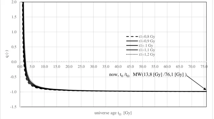
In the above equation, if the age of the universe is assumed to be 76,1 [Gy], then q= −0,986.

Figure 8: MW intrinsic velocity for t = 1 [Gy] to 76,1 [Gy]

0.0 100.0 200.0 300.0 400.0 500.0 600.0 700.0 1.0 6.0 11.0 16.0 21.0 26.0 31.0 36.0 41.0 46.0 51.0 56.0 61.0 66.0 71.0 76.0 v elo city [ k m /s ]

universe age t_(Gy)

46

Figure 9a:MW intrinsic acceleration for t = 1 [Gy] to 76,1 [Gy]

-1.4E-11 -1.3E-11 -1.2E-11 -1.1E-11 -1.0E-11 -9.0E-12 -8.0E-12 -7.0E-12 -6.0E-12 -5.0E-12 -4.0E-12 -3.0E-12 -2.0E-12 -1.0E-12 0.0E+00 1.0E-12 1.0 6.0 11.0 16.0 21.0 26.0 31.0 36.0 41.0 46.0 51.0 56.0 61.0 66.0 71.0 76.0 ac ce ler atio n [ m /s 2]

universe age t_[Gy]

47

Figure 10: MW intrinsic deceleration parameter for t = 1 [Gy] to 76,1 [Gy]

Figure 11:Masses deceleration parameter function of z

-1.5 -1.0 -0.5 0.0 0.5 1.0 1.5 2.0 0.0 5.0 10.0 15.0 20.0 25.0 30.0 35.0 40.0 45.0 50.0 55.0 60.0 65.0 70.0 75.0 q ( -)

universe age t [Gy]

t1=0,8 Gy t1=0,9 Gy t1= 1 Gy t1=1,1 Gy t1=1,2 Gy

now, t₀/t MW(13,8 [Gy] /76,1 [Gy] )

-2.0 -1.0 0.0 1.0 2.0 3.0 4.0 5.0 6.0 7.0 8.0 9.0 10.0 -1.0 0.0 1.0 2.0 3.0 4.0 5.0 6.0 7.0 8.0 9.0 10.0 11.0 12.0 13.0 q ( -) z (-)

measured (Sne Ia), Reiss et al.,1998, 0,16-z-0,62, q=-1 measured (Sne Ia), Kiselev, 0,05-z-0,85, q=-0,675 q(z), t1=1,0 Gy

now t₀(z=0) MW(13,8 Gy), univers age 76,1 Gy or z=-0,81, q= - 0,98