Coordination d'ordonnancement de production et de distribution

(1)

Universit´e Paris-Dauphine

´

Ecole doctorale de Dauphine

N◦ attribu´e par la biblioth`eque

Th`

ese

Pour l’obtention du grade de

Docteur en informatique

Coordination of production and

distribution scheduling

Coordination d’ordonnancement de production et de

distribution

Pr´esent´ee par : Liangliang FU

Soutenue le 2 d´

ecembre 2014 devant le jury compos´

e de :

Directeur de th`

ese :

Mohamed Ali ALOULOU Maˆıtre de conf´erences (HDR), Universit´e Paris-Dauphine

Rapporteurs :

Jean-Charles BILLAUT Professeur, Ecole Polytechnique de l’Université de Tours Safia KEDAD-SIDHOUM Maˆıtre de conférences (HDR), Université Pierre et Marie Curie

Examinateurs :

Stéphane DAUZ ÈRE-P ÉR ÈS Professeur, Ecole des Mines de Saint-étienne Ammar OULAMARA Professeur, Université de Lorraine

(2)

(3)

Abstract

In this dissertation, we aim at investigating three supply chain scheduling problems in the make-to-order business model. The first problem is a production and interstage dis-tribution scheduling problem in a supply chain with a manufacturer and a third-party logistics (3PL) provider. The second problem is a production and outbound distribution scheduling problem with release dates and deadlines in a supply chain with a manufac-turer, a 3PL provider and a customer. The third problem is a production and outbound distribution scheduling problem with setup times and delivery time windows in a sup-ply chain with a manufacturer, a 3PL provider and several customers. For the three problems, we study their individual scheduling problems and coordinated scheduling problems. We propose polynomial-time algorithms or prove the intractability of these problems, and develop exact algorithms or heuristics to solve the NP-hard problems. We establish mechanisms of coordination and evaluate the benefits of coordination.

Keywords: Supply chain scheduling, Coordination, Production and distribution schedul-ing, Dynamic programmschedul-ing, Branch-and-bound algorithm, Heuristic.

(4)

R´

esum´

e

Dans cette thèse, nous étudions trois problèmes d’ordonnancement de la chaˆıne logis-tique dans le modèle de production la demande. Le premier problème est un problème d’ordonnancement de production et de distribution intermédiaire dans une chaˆıne lo-gistique avec un producteur et un prestataire lolo-gistique. Le deuxième problème est un problème d’ordonnancement de production et de distribution aval avec des dates de début au plus tôt et des dates limites de livraison dans une chaˆıne logistique avec un producteur, un prestataire logistique et un client. Le troisième problème est un problème d’ordonnancement de production et de distribution aval avec des temps de réglage et des fenêtres de temps de livraison dans une chaˆıne logistique avec un produc-teur, un prestataire logistique et plusieurs clients. Pour les trois problèmes, nous étudions les problèmes d’ordonnancement individuels et les problèmes d’ordonnancement coor-donnés. Nous proposons des algorithmes polynomiaux ou prouvons la NP-complétude de ces problèmes, et développons des algorithmes exacts ou heuristiques pour résoudre les problèmes NP-difficiles. Nous proposons des mécanismes de coordination et évaluons le bénéfice de la coordination.

Mots cl´es: Ordonnancement de la chaˆıne logistique, Coordination, Ordonnancement de production et de distribution, Programmation dynamique, Algorithme B&B, Heuris-tique.

(5)

Acknowledgements

I would like to express my sincere gratitude to my supervisor Mohamed Ali Aloulou for his guidance, technical advice and enthusiastic support throughout my dissertation research. His wonderful patience and friendship encourage constantly my work. I am also extremely grateful to Daniel Vanderpooten for bringing me to the research and cultivating my interest in optimization. I would like to thank the members of jury, Jean-Charles Billaut, Stéphane Dauzère-pérès, Safia Kedad-sidhoum, Ammar Oulamara and Daniel Vanderpooten, for having accepted to evaluate the quality of my dissertation.

Next, my thanks are extended to Alessandro Agnetis, for his help on my research, invitation and especially the Italian dishes. I also want to thank Christian Artigues, Mikhail Y. Kovalyov and Chefi Triki, for their support on my research. A special thank you to Fran¸cois Herbinet for supporting my research on the real industry scheduling problem.

I wish to thank Florian, Renaud, Lyes, Edouard, Amine, Lydia and all other friends and colleagues at LAMSADE, for friendship, support and smile. Your kindness made my three years at Dauphine enjoyable and memorable.

I would like to thank my family with love. The deepest appreciation to my wife for her continued support and encouragement in the difficult periods. A kiss to my son for bringing me happy time everyday. Finally, I want to thank my parents for their patience, support and encouragement all the way.

(6)

List of Figures

3.1 Production-distribution schedule when manufacturer dominates, 3PL provider

adjusts . . . 32

3.2 Production-distribution schedule when 3PL provider dominates, Manu-facturer adjusts . . . 33

3.3 Illustration of property 4(a) of Lemma 3.1. . . 35

3.4 Illustration of Theorem 3.5. . . 50

3.5 Graphical representation of a delivery schedule . . . 51

3.6 Illustration of property 1 of Lemma 3.8. . . 62

4.1 Production-distribution schedule when manufacturer dominates, 3PL provider negotiates. . . 73

4.2 Production-distribution schedule when manufacturer and 3PL provider coordinate . . . 74

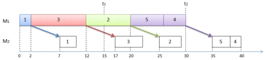
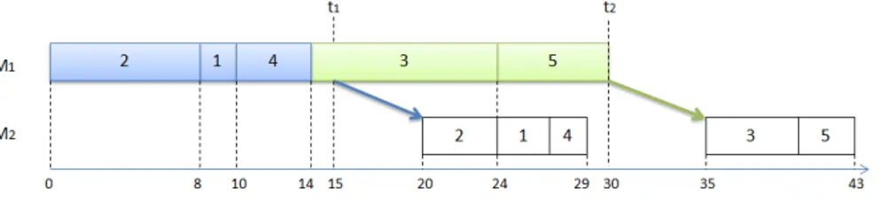
5.1 Optimal schedules for the integrated problems . . . 99

5.2 Schedules for the individual problems and the integrated problem . . . . 100

5.3 Illustration of property 1 of Lemma 5.3 . . . 108

5.4 Illustration of property 2 of Lemma 5.3 . . . 108

5.5 Illustration of branch-and-bound algorithm B5.1 . . . 117

5.6 An optimal solution for NSP-NSD problem . . . 119

6.1 Optimal production schedule without coordination . . . 132

6.2 Optimal production schedule with coordination . . . 132

(10)

List of Tables

3.1 Example for problem 1 . . . 32

3.2 Complexity of 3PL provider’s problem when manufacturer dominates and 3PL provider adjusts. . . 38

3.3 Complexity of 3PL provider problems when 3PL provider dominates and manufacturer adjusts. . . 59

4.1 Average computational times of execution of algorithms. . . 88

4.2 Failure rates and relative gaps of MILP. . . 88

4.3 Benefits of coordination in scenario (4) . . . 88

4.4 Price of dominance for 3PL provider. . . 89

4.5 Benefits of coordination in scenario (4) under various experiment aggre-gations. . . 89

4.6 Benefit of relaxing responsiveness constraints in scenario (3). . . 90

5.1 Example for the integrated problems . . . 99

5.2 Example for evaluation of the benefit of coordination . . . 100

5.3 Example for branch-and-bound algorithm B5.1 . . . 116

5.4 Performance of branch-and-bound algorithm B5.1. . . 123

5.5 Performance of two MILP models. . . 123

5.6 Gaps of solutions of branch-and-bound algorithm B5.1. . . 124

5.7 Gaps of solutions of two MILP models. . . 124

6.1 Average computational times of execution of heuristic . . . 143

6.2 Benefit of coordination . . . 143

(11)

Chapter 1 Introduction

1.1 Background

A supply chain involves a set of organizations, including suppliers, manufacturers, lo-gistics providers, distributors and retailers, who work together to satisfy customers’ demands. The cost of a product includes the cost of resources at all stages, such as pro-curement of raw materials, production, distribution of finished products to customers. The objective of supply chain management is to incorporate activities across organiza-tions for adding value, reducing cost and increasing customer service quality. Thomas and Griffin (1996) provided a literature review on supply chain management.

In recent decades, globalization expands supply chain over national boundaries and brings a fierce competition market. In order to satisfy customers’ heightened expecta-tions, the enterprises increasingly find that they must rely on effective supply chains. A non-efficient supply chain may carry a high cost. For example, the logistics market volume in Europe accounted in 2012 for 930 billion euros (Kille and Schwemmer 2013). The weight of transportation sector is around 44% of added value and 48% of total em-ployment. According to Eurostat data 2012 (Palmer et al. 2012), third party logistics (3PL) providers fail to consolidate their customers’ transport orders: about 24% of all road freight kilometers driven in Europe are empty vehicles and the average vehicle is loaded to 56% of its capacity in terms of weight.

As production and distribution are the main business processes in supply chain, the coordination of production and distribution issue is crucial in supply chain management.

(12)

1.1. Background 2

In traditional supply chain, production and distribution are separated by a large in-termediate inventory and are planned independently. This independence can simplify decision-making but increases the holding inventory cost. Facing the fierce competition at current internal market and the expectations of customers, many enterprises adopt the make-to-order (a.k.a. assemble-to-order, build-to-order) business model. These en-terprises include the ones with highly configured product as automobiles, computers, or with expensive inventory as aircraft. In this context, a product starts to be built after the order is received and there is a small or zero intermediate inventory between production and distribution. Consequently, the coordination of production and distri-bution is required in this business model. This coordination is also essential in supply chains with time-sensitive products as food, ready-mix concrete paste and newspapers. These products should be delivered to customers immediately or a short time after their production.

In the research literature on supply chain management, coordination issues at the strategic and tactical levels have attracted an extensive research. The issues at the strategic level focus on long-term decision-making, such as allocation of manufacturing equipment, plant opening, selection of distribution centers, etc. Research at the tactical level is targeted at medium-term decision-making, such as planning of production, inven-tory and distribution in a time period like one year, etc. The issues at the operational level have been investigated during the last decade and are always under developing. They focus on the order-by-order scheduling decision-making, such as machine schedul-ing, batch delivery, vehicle routschedul-ing, etc. My thesis addresses the need of research at the operational level pointed out by Thomas and Griffin (1996) .

The coordination model varies with the supply chain models. With the develop-ment of the data exchange technology, especially the introduction of enterprise resource planning (ERP) systems and Internet-based collaborative systems, the supply chain can integrate the key business processes for adding value and saving cost. In this integrated supply chain, the involved organizations often belong to one corporation and work in collaborative relationship. In this model, the coordination is controlled by the corpora-tion and the goal is to optimize the performance of the global supply chain. From 1990, some enterprises abandoned the integration and focused on their core competencies and

(13)

1.1. Background 3

specialization. They outsource the non-core operations to other enterprises for improv-ing their efficiency. Accordimprov-ing to the European commission 2011, in 2010, the share of own-account transport is around 15% of the tonne-km generated in road freight trans-port. This means that transport is mostly outsourced to independent partners like Third Party Logistics (3PL) providers. In this non-integrated supply chain, the independent enterprises have their own objectives and accept the coordination only if they can benefit from it. A negotiation-based mechanism is necessary to motivate the coordination.

The integrated production and distribution scheduling (IPDS) issue, motivated by the integrated supply chain, has been investigated from 1980. This issue investigates the integration of production scheduling decision-making and distribution decision-making at the operational level. Chen (2010) provided an extensive review of the literature on the integrated production and outbound distribution scheduling (IPODS) problems. Outbound distribution deals with a manufacturer shipping his products to the next stage of the supply chain, that typically belongs to another company. As a conse-quence, the receiving firm may set due dates or deadlines that will constrain the pro-duction/distribution problem. The focus of the analysis is on coordinating production decisions (typically, sequencing) and distribution decisions (typically, batching). These two aspects are often conflicting, and require a careful consideration of objectives and roles of the subjects involved. A few articles address the integrated production and in-terstage distribution scheduling (IPIDS) issues. In most of papers studying IPDS issue, they did not evaluate the benefit of coordination by comparing the integrated solution with the non-coordinated solution. Since the solution of IPDS problems can also be used in the non-integrated supply chain with a compensation mechanism, the IPDS issue is also importance for the non-integrated supply chain.

The term supply chain scheduling was mentioned, by Dawande et al. (2006) , to define the coordination of scheduling decisions at the operational level. Several subproblems are investigated in this respect:

the individual scheduling problems without coordination, where the decision maker optimizes his individual schedule subject to the constraints imposed by the other decision maker in the supply chain;

(14)

1.2. Contribution 4

jointly their schedules;

the mechanism of coordination explaining how the decision makers coordinate their activities;

the evaluation of the benefit of coordination.

Some researches addressing this need have been made in the last decade. For example, Hall and Potts (2003) investigated coordinated scheduling problems between the suppli-ers and the manufactursuppli-ers in a three stage supply chain. Dawande et al. (2006) studied the coordination between a manufacturer and a distributor in different bargaining powers scenarios.

1.2 Contribution

In this dissertation, we aim at investigating three supply chain scheduling problems in the make-to-order business model. The research objectives are to:

study the individual scheduling problems and coordinated scheduling problems: – propose polynomial-time algorithms for some polynomial-time solvable

prob-lems,

– prove the intractability for some NP-hard problems,

– develop exact algorithms or heuristics to solve the NP-hard problems; establish mechanisms of coordination;

evaluate the benefit of coordination. We consider the following scheduling problems:

Problem 1: production and interstage distribution scheduling problem (Ag-netis et al. 2014a, 2014b, 2014c)

In this problem, we consider a supply chain with a manufacturer and a 3PL provider. The manufacturer has to process a set of orders on one machine at upstream and down-stream stages. We consider the permutation flow shop environment in production. The 3PL provider is in charge of transportation of semi-finished products from the upstream

(15)

1.2. Contribution 5

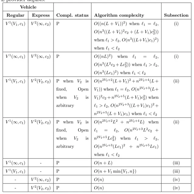
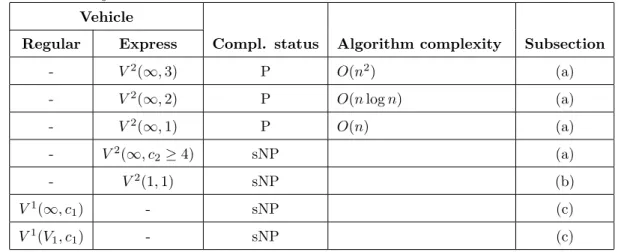
stage to the downstream stage. A batch cannot be delivered until all orders of the batch are completed at the upstream stage. Two transportation modes are considered: regular transportation, for which delivery departure times are fixed, and express transportation, for which delivery departure times are flexible. The manufacturer’s objective is to min-imize the makespan and the 3PL provider’s objective is to minmin-imize the transportation cost. We investigate four scenarios: (1) manufacturer dominates, 3PL provider adjusts; (2) 3PL provider dominates, manufacturer adjusts; (3) manufacturer dominates, 3PL provider negotiates; (4) manufacturer and 3PL provider coordinate. For the scheduling problems in each scenario, we provide polynomial-time algorithms or prove their NP-completeness. We provide two mechanisms of coordination for scenarios (3) and (4) and evaluate the benefit of coordination using numerical experiments.

Problem 2: production and outbound distribution scheduling problem with release dates and deadlines (Fu et al. 2014)

In this problem, we consider a supply chain with a manufacturer, a 3PL provider and a customer. The manufacturer has to process a set of orders on one machine, then the 3PL provider delivers them in batches to the customer. Each order has a release date and a delivery deadline fixed by the customer. The manufacturer’s objective is to ensure that all orders are delivered before or at their deadline and the 3PL provider’s objective is to minimize the transportation cost. We first investigate individual scheduling problems. Then we consider three coordinated scheduling problems with different ways how an order can be produced and delivered: non-splittable production and delivery (NSP-NSD) problem, splittable production and non-splittable delivery (SP-(NSP-NSD) problem and splittable production and delivery (SP-SD) problem. For these scheduling problems, we provide a polynomial-time algorithm for some restricted versions of SP-NSD and SP-SD problems and a branch-and-bound algorithm for NSP-NSD problem which is NP-hard. We evaluate the performance of branch-and-bound algorithm using numerical experiments.

Problem 3: production and outbound distribution scheduling problem with setup times and delivery time windows

This problem is a real problem proposed by a company working in the packaging industry. We consider a supply chain with a manufacturer, a 3PL provider and several customers.

(16)

1.3. Organization of the dissertation 6

The manufacturer has to process a set of orders on unrelated parallel machines and splitting of order is allowed in production. A sequence-dependent setup time and a setup cost occur when production changes from one order to another order. Then the 3PL provider delivers orders in batches to the customers with heterogeneous vehicles subject to delivery time windows. The manufacturer’s objective is to minimize the total setup cost and the 3PL provider’s objective is to minimize the transportation cost. We propose mathematical models for individual scheduling problems and coordinated scheduling problem. We develop a first decomposition approach to solve the coordinated scheduling problem using a commercial solver. we evaluate the feasibility of the approach and the potential benefit of coordination using numerical experiments for small instances. Finally, we propose some directions of improvement for further research.

1.3 Organization of the dissertation

This dissertation is organized as follows. Chapter 2 is dedicated to a literature review on production scheduling, distribution scheduling, integrated production and distribution scheduling, and supply chain scheduling. The three investigated problems are presented in two parts. In part I, we investigate a production and interstage distribution schedul-ing problem, i.e., the problem 1, which is divided to be presented in chapter 3 and chapter 4. In chapter 3, we study the individual scheduling problems, i.e., scenarios (1) manufacturer dominates, 3PL provider adjusts and (2) 3PL provider dominates, manu-facturer adjusts. In chapter 4, we study the coordinated scheduling problems in different scenarios, i.e., scenarios (3) manufacturer dominates, 3PL provider negotiates and (4) manufacturer and 3PL provider coordinate. Then, we evaluate the benefit of coordi-nation using numerical experiments. In part II, we investigate the two production and outbound distribution scheduling problems, i.e., problem 2 and problem 3, which are studied respectively in chapter 5 and chapter 6. Chapter 7 contains conclusions and perspectives of future research.

(17)

Chapter 2 Literature Review

In this chapter, we provide a literature review on the following problems: production scheduling, distribution scheduling, integrated production and distribution scheduling, and supply chain scheduling.

2.1 Production scheduling

Production scheduling problem can be presented generally as follows: supposing that a set of orders have to be processed on a set of machines, the problem is how to allocate one or more time intervals for each order to one or more machines while optimizing one or several objective functions.

Graham et al. (1979) introduced a three-field classification α|β|γ for production scheduling problem, where α, β and γ specify respectively machine environment, or-der characteristics and optimality criteria. This classification was extended by Brucker (2007).

The machine environment is specified by a string α = α1α2. α2 denotes the number

of machines. If α1 ∈ {◦, P , Q, R, P M P M , QM P M }, then each order consists of a

single operation. If α1 ∈ {G, J, F , O, X}, then each order consists of a set of operations.

If α1 ∈ {M P T }, then each order requires one or more processors at a time. The values

are characterized as:

α1 = ◦: single machine;

(18)

2.1. Production scheduling 8 α1 = P : identical parallel machines, i.e., processing speeds of machines are

identi-cal;

α1 = Q: uniform parallel machines, i.e., processing speeds of machines are

machine-dependent;

α1 = R: unrelated parallel machines, i.e., processing speeds of machines are

machine-dependent and order-dependent;

α1 = P M P M : multi-purpose identical parallel machines, i.e., an operation can be

processed on any machine equipped with the appropriate tool, and the machines are identical;

α1 = QM P M : multi-purpose identical parallel machines, i.e., an operation can be

processed on any machine equipped with the appropriate tool, and the machines are uniform; α1 = G: general shop; α1 = J : job shop; α1 = F : flow shop; α1 = O: open shop; α1 = X: mixed shop;

The order characteristics are specified by β ⊆ {β1, β2, . . ., β7}. The values are

characterized as:

β1 ∈ {pmtn, split}, i.e., preemption or splitting of order is allowed, and in the

splitting environment the split order can be processed simultaneously on several machines, which is different from the preemption environment;

β2 = prec, i.e., precedence relations exist between the orders;

β3 = rj, i.e., orders may have different release dates from which their production

(19)

2.1. Production scheduling 9 β4 specifies the restrictions on processing times or number of operations;

β5 = dj, i.e., orders may have different deadlines;

β6 ∈ {p − batch, s − batch}, i.e., orders can be scheduled in batches, the length of a

batch is equal to the maximum (sum) of processing times of all orders in the batch for p-batching (s-batching) problem;

β7 ∈ {sj, sij, sijk}, i.e., a setup time occurs when the production changes from

a family (or order) to another family (or order), sj and sij represent

sequence-independent setup time and sequence-dependent setup time respectively, and sijk

represent sequence-dependent and machine-dependent setup time.

The optimality criteria are commonly specified by the total cost objectives depending on completion times of orders, and the customer service quality objectives depending on due dates of orders. The objectives are characterized by two types of functions: the bottleneck objectives, as makespan Cmax, maximum lateness Lmax; the sum objectives,

as (weighted) total flow time, (weighted) total tardiness, (weighted) total earliness, etc. The objective of scheduling problem is to minimize one or several objective functions.

Production scheduling problem has been extensively investigated from the mid 1950s. In the book of Brucher (2007), he discussed the classical scheduling algorithms for solving single machine scheduling problems, parallel machine scheduling problems, shop schedul-ing problems, due dates schedulschedul-ing problems, batchschedul-ing problems, schedulschedul-ing problems with setup times, multi-purpose machines problems and multiprocessor tasks scheduling problems.

In the following, we focus on the literature of some problems linked to our research: flow shop scheduling problems, single machine scheduling problems with release dates, and scheduling problems with setup times.

In flow shop scheduling problems, each order has to be processed in a fixed sequence of machines, i.e., the first operation of each order is performed on the first machine, the second operation on the second machine, and so on. For regular objective functions, i.e., functions that are non-decreasing in completion times of orders, the problem is to find a processing sequence of orders for each machine. We focus on some flow shop scheduling

(20)

2.1. Production scheduling 10

problems with makespan objective function Cmax. Johnson (1954) provided a

polynomial-time algorithm to solve the 2-machine flow shop scheduling problem F 2||Cmax. Garey

et al. (1976) proved the NP-hardness of the m-machine flow shop scheduling problem F m||Cmax with m ≥ 3.

Concerning the single machine scheduling problems with release dates, we focus on the problems with maximum lateness Lmax objective function. The problem without

release dates 1||Lmaxcan be solved by Jackson’s earliest due date (EDD) rule introduced

by Jackson (1955). This problem is a special case of the problem 1|prec|Lmaxsolved by a

polynomial-time algorithm provided by Lawler (1973). The problem with release dates and preemption 1|rj, pmtn|Lmaxcan be solved by Jackson’s preemptive earliest due date

(EDD-preemptive) rule introduced by Jackson (1955). This problem is a special case of the problem 1|prec, rj, pmtn|Lmax solved by a polynomial-time algorithm provided

by Baker et al. (1983). Lenstra et al. (1977) proved the NP-hardness of the problem 1|rj|Lmax. Carlier (1982) provided the first efficient branch-and-bound algorithm to solve

this problem.

Allahverdi et al. (2008) provided a survey of scheduling problems with setup times or costs. They discussed the problems with sequence-independent setup time (sj) or

sequence-dependent setup time (sij). sj depends upon only order j processed after

the changeover, while sij depends upon both orders i and j processed before and after

the changeover respectively. We focus on the problems with the objective of minimiz-ing makespan Cmax or sum of setup cost. The single machine problem 1|sj|Cmax is

polynomial-time solvable. The single machine problem 1|sij|Cmax is NP-hard (Bruno

and Downey 1978) and can be reformulated as a Traveling Salesman Problem (TSP). The two parallel machine problem with unit processing times and unit setup times P 2|pj = 1; sj = 1|Cmax is NP-hard (Brucker et al. 1998). The special case of this

problem where all families have equal sizes can be solved in polynomial time (Brucker 2007). Several heuristics and meta-heuristics were provided for the parallel machine problem P 2|sij|Cmax: a divide and merge heuristic by Gendreau et al. (2001), a

heuris-tic and a tabu search algorithm by Mendes et al. (2002), and a hybrid meta-heurisheuris-tic by Behnamian et al. (2009). For the same problem with splitting of order, in that orders can be split and processed simultaneously on different machines, some heuristics were

(21)

2.2. Distribution scheduling 11

provided by Tahar et al. (2006) and Yalaoui and Chu (2003). Concerning the problems with the sum of setup cost objective function, few papers have investigated this problem. Miller et al. (1999) provided a hybrid genetic algorithm for a single machine scheduling problem with sequence-dependent setup time minimizing the sum of setup cost, inventory cost, and backlog cost. Vignier et al. (1999) considered a parallel machines scheduling problem with sequence-dependent setup time, release dates and deadline. The objec-tive function is to first find a feasible schedule and then to minimize the cost due to assignment and setup time costs. They proposed a hybrid method that consists of an iterative heuristic, a genetic algorithm, and a branch-and-bound algorithm. Anglani et al. (2005) proposed a fuzzy mathematical programming approach to solve a parallel machines scheduling problem with sequence-dependent setup time, uncertain processing time and the objective of minimizing the total setup costs.

Some other scheduling problems with setup times have been investigated, such as flow shop scheduling problems with setup times (Cheng et al. 1999, Brucker et al. 2005, etc.), open shop scheduling problems with setup times(Averbakh et al. 2005, Billaut et al. 2008, etc.), job shop scheduling problems with setup times (Cheung and Zhou 2001, Artigues and Roubellat 2002, etc.).

2.2 Distribution scheduling

Distribution scheduling problem is a central problem in distribution management and is faced by a lot of enterprises every day. There are three types of delivery (Chen 2010): individual delivery, i.e., each order is shipped individually; direct batch delivery, i.e., different orders of a customer can be delivered together in a shipment; routing batch delivery, also named as vehicle routing delivery, i.e., orders of different customers can be delivered together in a shipment. The individual delivery and direct batch delivery are used to deliver the time-sensitive products. The vehicle routing delivery is extensively adopted by many enterprises to reduce distribution cost. In the literature on distribution management, the vehicle routing problem has attracted an extensive research since the first study provided by Dantzig and Ramser (1959). In fact, the first two types of delivery can be seen as two special cases of the vehicle routing delivery. There are few

(22)

articles investigating only the distribution scheduling problem with the first two types of delivery. In many cases, these problems are simple and have been discussed in the integrated production and distribution scheduling problems (Chen 2010). However, it is interesting to investigate these problems with some adding characteristics, such as a limited number of vehicles, vehicles with fixed departure dates, heterogeneous vehicles, release dates, delivery deadlines, etc. In this section, we focus on vehicle routing problem. The classical vehicle routing problem (VRP) is to determine a set of routes for a fleet of vehicles, each of which starts and ends at its own depot, to serve a set of customers on minimizing the total travel cost subject to a set of constraints. The VRP is one of the most popular combinatorial optimization problems and is NP-hard because it generates the traveling salesman problem (TSP) (Dantzig and Ramser 1959). A lot of exact algo-rithms and heuristics are provided to solve the VRP. Toth and Vigo (2002) surveyed the variants of the VRP. The capacitated vehicle routing problem (CVRP) considers the ve-hicle capacity. In the distance-constrained veve-hicle routing problem (DVRP), the length of each each route cannot exceed a preset limit. The capacitated distance-constrained vehicle routing problem (DCVRP) considers both the vehicle capacity and the constraint of distance. In the vehicle routing problem with time windows (VRPTW), the service at each customer must start within a given time window and the arrival of vehicles after time windows are prohibited. In the vehicle routing problem with backhauls (VRPB), each customer location may act as a pickup or a delivery node and all deliveries must be performed before any pickup. In the vehicle routing problem with pickup and de-livery (VRPPD), the passengers or goods are transported between pickup and dede-livery locations. All the above problems are NP-hard because they generate the classical VRP. Toth and Vigo (2002) provided a survey of exact algorithms and heuristics for all the above vehicle routing problems. Similar surveys were provided in chapter 6 (Cordeau et al. 2007) and chapter 7 (Cordeau et al. 2007) of the handbook of operations research and management science. Other surveys have been provided for one or some of the above problems, such as VRPTW by Br¨aysy and Gendreau (2005), VRPB and VRPPD by Parragh et al. (2008), large-scale VRPTW by Gendreau and Tarantilis (2010), CVRP and VRPTW by Kumar and Panneerselvam (2012). There are other variations of the VRP, such as the dynamic vehicle routing problem (DVRP) where part or all of the

(23)

input is unknown before the start of working day, the heterogeneous fleet vehicle routing problem (HVRP) where a fleet of vehicles is characterized by different capacities and costs, and the split delivery vehicle routing problem (SDVRP). Surveys on DVRP, HVRP and SDVRP were provided respectively by Pillac et al. (2013), Baldacci et al. (2008) and Archetti and Speranza (2008).

In the following, we focus on the exact algorithms and heuristics for the VRPTW. The VRPTW can be defined on a directed graph and formulated as a multicommodity network model with time windows and capacity constraints (Desrochers et al. 1988). There are four main exact algorithms for the VRPTW: Lagrangian relaxation based branch-and-bound algorithm where the lower bound is obtained by Lagrangian relax-ation (Fishier 1994, Fishier et al. 1997, Kohl and Madsen 1997, Kallehauge et al. 2006); column generation based branch-and-bound algorithm where the linear relaxations are solved by column generation (Desrochers et al. 1992, Kohl et al. 1999, Cook and Rich 1999); branch-and-cut algorithm where the upper bound is obtained by a greedy ran-domized adaptive search procedure (Bard et al. 2002); genetic and set partitioning two-phase approach (Alvarenga et al. 2007). Because of the NP-hardness of the VRPTW, the research has concentrated on heuristics, such as construction heuristics where at a time one customer is inserted into partial routes until a feasible solution is obtained (Solomon 1987, Potvin and Rousseau 1993, Ioannou et al. 2001, Nagata and Bräysy 2009, Pang 2011), improvement heuristics where a feasible solution is improved itera-tively with an exchange mechanism (Russell 1977, Baker and Schaffer 1986, Potvin and Rousseau 1995, etc.), combination of construction and improvement heuristics (Russell 1995, Cordone and Wolfler Calvo 2001, Bräysy 2002), tabu search heuristics (Taillard et al. 1997, Chiang and Russell 1997, Cordeau et al. 2001, Lau et al. 2003, etc.), ge-netic algorithms (Gehring and Homberger 2002, Berger et al. 2003, Mester and Bräysy 2005, etc.), two-phase greedy randomized adaptive search procedure (Kontoravdis and Bard 1995), guided local search algorithm (Kilby et al. 1999), ant colony optimization algorithm (Gambardella et al. 1999), four-phase metaheuristic (Bräysy 2003), two-stage hybrid algorithm (Bent and Van Hentenryck 2004), improved multi-objective evolution-ary algorithm (Garcia-Najera and Bullinaria 2011), etc.

(24)

2.3. Integrated production and distribution scheduling 14

2.3 Integrated production and distribution

schedul-ing

In the literature, two types of integrated production and distribution scheduling problems have been investigated: the integrated production and interstage distribution scheduling (IPIDS) problem involving the distribution of orders between manufacturing stages in the shop production, such as flow shop, job shop, open shop, etc; the integrated production and outbound distribution scheduling (IPODS) problem involving the distribution of orders to the customers.

In the IPIDS problem, the production and transportation of orders between the stages are taken into account. The problem can be specified by the characteristics of ma-chine environment, i.e., flow shop, job shop, open shop and so on, by the characteristics of transportation time, i.e., order-dependent, order-independent, machine-dependent, machine-independent and constant, by the characteristics of transporters, i.e., sufficient number, limited number, unlimited capacity and limited capacity. Brucker et al. (2004) provided a survey on the IPIDS problem in the flow shop and open shop environments. There are other surveys in the literature on the IPIDS, such as Hurinka and Knustb (2001), and Lee and Chen (2001).

We focus on the IPIDS problems with order-independent transportation time in 2-machine flow shop. Here, we use the three-field classification α|β|γ of production schedul-ing problem for the IPIDS problems. Maggu and Das (1980) developed a polynomial time algorithm based on well-known Johnson’s rule (Johnson 1954) for the problem of minimizing the makespan subject to an unlimited number of transporters with order-dependent transportation time, denoted by F 2|tj, v ≥ n|Cmax, where tj, v and n represent

respectively order-dependent transportation time, number of transporters and number of orders. Since the problem with order-independent transportation time can be seen as a special case of the problem with order-dependent transportation time, the similar problem with order-independent transportation time F 2|tj ∈ {t1, t2}, v ≥ n|Cmax can

be solved by the same algorithm, where t1 represents the transportation time from the

first stage to the second while t2 represents the returning time. The problem minimizing

(25)

transportation time, denoted by F 2|tj ∈ {t1, t2}, v = 1, c = 1|Cmax was proved to be

strongly NP-hard even if t1 = t2 (Hurinka and Knustb 2001). Tang et al. (2010)

devel-oped an approximation algorithm with worst case ratio of 2 for this problem. Lee and Chen (2001) proved the NP-hardness of a similar problem with a vehicle capacity more than 2, denoted by F 2|tj ∈ {t1, t2}, v = 1, c ≥ 3|Cmax, and provided a polynomial-time

dynamic programming algorithm for the special case with equal processing times on one machine and a fixed number of vehicles. Lee and Strusevich (2005) proved that for the problem F 2|tj ∈ {t1, t2}, v = 1, c ≥ n|Cmax, finding the best schedule in class SF (2) of

schedules with at most two shipments is NP-hard even if t1 = t2, and provided an

ap-proximation algorithm with worst case ratio of 3/2, which is the best possible algorithm in the class of heuristics that construct schedules with at most two shipments. Gong and Tang (2011) developed an approximation algorithm with worst case ratio of 2 for the problem F 2|tj ∈ {t1, t2}, v = 1, c ≥ n|Cmax and an approximation algorithm with worst

case ratio of 7/3 for a similar problem with the orders having different sizes of physical storage space in the transporter. There are also other related problems with buffer space constraints studied by Stern and Vitner (1990), Panwalkar (1991).

While the above articles considered transportation capacity and transportation time, few articles consider transportation cost. As mentioned in previous chapter, in a global supply chain, a product can be processed at different plants located at different geo-graphic locations. So the transportation cost is not negligible. Aloulou et al. (2014) considered a bicriteria 2-machine flow shop serial-batching scheduling problem with a sufficient number of transporters with limited capacity. They developed two approx-imation algorithms and provided polynomial-time algorithms for some special cases. They considered two criteria: number of production batches and makespan. This prob-lem is equivalent to the probprob-lem F 2|tj ∈ {t1, t2}, v ≥ n, c ≥ 1|T C, Cmax, where T C

represents the trip-based transportation cost, where the cost of one delivery batch is order-independent.

Chen (2010) surveyed the IPODS problems and introduced a five-field notation, α|β|π|δ|γ, to represent the IPODS models. α, β and γ specify respectively the ma-chine environment, the order characteristics and the optimality criterion as the classical three-field classification (Graham et al. 1979, Pinedo 2002). Some new objective

(26)

func-2.3. Integrated production and distribution scheduling 16

tions of transportation are introduced, such as maximum delivery time denoted by Dmax,

total trip-based transportation cost denoted by T C, etc. π and δ specify respectively the characteristics of delivery process and the number of customers. The number of customers is specified by one value of {1, k, n}, where δ = k ≥ 2 means there are mul-tiple customers, and δ = n means that each order belongs to a different customer. The characteristics of delivery process include vehicle characteristics (number and capacity of vehicles) and delivery methods. The vehicle characteristics are specified by V (x, y), where:

x ∈ {1, v, ∞} represents the number of vehicles.

y ∈ {1, c, ∞, Q} represents the capacity of vehicles. {1, c, ∞} and Q distinguish, respectively, the possible capacities of vehicles when orders have equal size, and the limited capacity of vehicles when orders have general size.

The delivery methods include:

iid: individual and immediate delivery. direct: direct batch delivery.

routing: batch routing delivery.

fdep: shipping with fixed delivery departure dates.

split: splittable delivery, i.e., an order can be split and delivered by several vehicles. The IPODS problems are classified by delivery methods: (i) models with individual and immediate delivery; (ii) models with direct batch delivery to a single customer; (iii) models with batch routing delivery to multiple customers; (iv) models with batch routing delivery to multiple customers; (v) models with fixed delivery departure dates. Chen (2010) surveyed the algorithms, heuristics, and complexity for the IPODS problems in each class.

We focus on the IPODS problems related to our considered problems: the IPODS problems with release dates rj; the IPODS problems with maximum lateness Lmax or

delivery deadline dj, and transportation cost T C; the IPODS problems with setup times

(27)

P m|rj|V (∞, 1), iid|n|Dmax, (iv) F m|rj|V (∞, 1), iid|n|Dmax are strongly NP-hard. Liu

and Cheng (2002) proved the NP-hardness of the problem (v) 1|rj, sj, pmtn|V (∞,

1), iid|n|Dmax. In these problems, the orders are delivered individually and

imme-diately to the customers upon their completion while minimizing the maximum de-livery time. For problems (i), (ii), (iii) and (v), approximation algorithms and (or) polynomial-time approximation schemes were provided by Potts (1980), Hall and Shmoys (1989, 1992), Mastrolilli (2003), Zdrzalka (1994), Liu and Cheng (2002). Gharbi and Haouari (2002) developed a branch-and-bound algorithm for problem (iii). Kamin-sky (2003) proposed an asymptotic optimality of the longest delivery time algorithm for problem (iv). Few articles consider direct or routing delivery. Lu et al. (2008) provided a polynomial-time algorithm for the problem 1|rj, pmtn|V (1, c), direct|1|Dmax.

For the problem 1|rj|V (1, c), direct|1|Dmax they proved its NP-hardness and proposed

an approximation algorithm with worst case ratio of 5/3. Mazdeh et al. (2008) provided a branch-and-bound algorithm for a special case of the NP-hard problem 1|rj|V (∞, ∞), direct|n|P Fj+ T C, where P Fj represents the total flow time. Mazdeh

et al. (2012) provided a branch-and-bound algorithm for a special case of the similar problem with sum of weighted flow time, 1|rj|V (∞, ∞), direct|n|P wjFj + T C.

Sel-varajah et al. (2013) provided an evolutionary meta-heuristic for the same problem in the general case and a polynomial-time algorithm for the special case with common weight and preemption in production, 1|rj, pmtn|V (∞, ∞), direct|n|P wFj + T C and

1|rj, pmtn| V (∞, ∞), direct|n|P wCj+ T C. There are some articles considering the

on-line problem, i.e., the information related to an order becomes known when this order is released. Ng and Lu (2012) investigated the problems of Lu et al. (2008) in on-line envi-ronment. Averbakh and Xue (2007) provided an on-line two-competitive algorithm for the on-line problem 1|rj, pmtn|V (∞, ∞), direct|k|P Dj + T C, where P Dj represents

(28)

IPODS problems with Lmax and T C: Some IPODS problems with maximum

lateness Lmax or delivery deadline dj, and transportation cost T C have been

inves-tigated in the literature. Polynomial-time algorithms were provided for the prob-lems 1||V (∞, ∞), direct|k|Lmax + T C with a fixed k by Hall and Potts (2003),

1||V (∞, c), direct|k|Lmax+ T C with a fixed k by Pundoor and Chen (2005), 1||V (1, ∞),

direct|1|Lmax + T C by Hall and Potts (2005), 1||V (v, ∞), direct|1|Lmax + T C with

a fixed v and 1||V (1, ∞), routing|k|Lmax + T C with a fixed k by Chen (2010),

1|pmtn, dj|V (∞, Q), direct|1|T C by Chen and Pundoor (2009). Wang and Lee (2005)

proved the NP-hardness of the problem 1|dj|V (∞, 1), iid|n|T C with two types of vehicles

and provided a pseudo-polynomial time dynamic programming algorithm for a special case. Chen and Pundoor (2009) proved the NP-hardness of the problems without pre-emption of production, 1|dj|V (∞, Q)|1|T C and 1|dj|V (∞, Q), direct|1|T C, and provided

approximation algorithms with worst-case ratio of 2.

IPODS problems with setup times: Few articles investigated the IPODS problem with sequence-independent setup times (sj) or sequence-dependent setup times (sij). The

problem with sequence-independent setup time and individual and immediate delivery, 1|sj|V (∞, 1), iid|n| Dmax, is strongly NP-hard (Chen 2010). Zdrzalka (1991) provided

an approximation algorithm with worst case ratio of 5/3 for the problem in the case with unit setup times, and Zdrzalka (1995) provided an approximation algorithm with worst case ratio of 3/2 for the problem in the case with general setup times. Woeg-inger (1998) developed a polynomial-time approximation scheme for this problem. Liu and Cheng (2002) proved the NP-hardness and provided a polynomial-time approxi-mation scheme for the similar problem with release dates and preemption of produc-tion, 1|rj, sj, pmtn|V (∞, 1), iid|n|Dmax. Zdrzalka (1994) provided an approximation

with worst case ratio of 3/2 for this problem. Van Buer, et al. (1999) proved the NP-hardness and provided a heuristic for the problem with sequence-dependent setup time and routing delivery, 1|sij, dj|V (∞, Q), routing|n|T C + V C, where T C and V C

repre-sent respectively the trip-based transportation cost and the vehicle-based transportation cost. Wang and Cheng (2009) provided three heuristics for the NP-hard problem with sequence-dependent setup times and direct delivery, P 2|sj|V (∞, c), direct|k|Dmax+ T C.

(29)

2.4. Supply chain scheduling 19

IPODS problems with routing delivery and time windows: While the

VRPTW has been well studied, few articles investigated the IPODS problem with routing delivery and time windows. Ullrich (2013) investigated the problem P m, rm|[aj, bj]|V (v, Q), routing|k|P Tj, i.e., a set of orders of general size is processed

on parallel machines subject to the machine release time rm, and delivered to customers

within the time windows [aj, bj] by a fleet of heterogeneous vehicles on minimizing the

sum of tardinessP Tj. They provided a genetic algorithm for the integrated problem and

evaluated its performance by comparing with two classical decomposition approaches. Low et al. (2014) provided an integer nonlinear programming model and two adap-tive genetic algorithms for the problem 1|[aj, bj]|V (∞, Q), routing|n|T C +P Ej+P Tj,

where retailers’ orders are processed in a distribution center and delivered to customers by a fleet of heterogeneous vehicles within the soft time windows, i.e., the violation of time windows incurs a penalty. The objective is to minimize the total cost includ-ing the transportation cost, the penalty cost of earliness P Ej and the penalty cost of

tardiness P Tj. Low et al. (2013) investigated the problem with the same model on

minimizing the time required to complete producing the product, delivering it to re-tailers and returning to the distribution center. Chen (2009) investigated an IPODS problem with routing delivery and time windows for perishable food products, which cannot be represented by the five-field notation of Chen (2010). In this problem, the products of each delivery batch are produced continuously on a single machine and are delivered to customers within soft time windows. The orders are assumed stochastic and the deterioration of products throughout their lifetime is considered. The objective is to maximize the expected total profit of the supplier. He proposed an algorithm composed of the constrained Nelder-Mead method (Nelder and Mead 1965) and a heuristic for the VRPTW.

2.4 Supply chain scheduling

As mentioned in the previous chapter, the supply chain scheduling problem focuses on the coordination of the scheduling decisions (Dawande et al. 2006). Generally, the following problems are considered: the individual scheduling problems at the conflict models, the

(30)

coordinated scheduling problem and the mechanisms of coordination, and the evaluation of the benefit of coordination. Since it is difficult to consider the coordination in the whole supply chain, the coordination between two or three stages has been considered in several articles.

Hall and Potts (2003) were the first to study supply chain scheduling problems. In their model, a three-stage supply chain is formed by suppliers, manufacturers, and customers. A supplier makes deliveries to several manufacturers who also make deliveries to customers. The problems in each stage have been studied. From the viewpoint of the supplier, the problem is to minimize the sum of production and delivery costs, where three production costs are considered respectively: sum of flow times, maximum lateness and number of late orders. From the viewpoint of the one manufacturer, the problem is to minimize the sum of production and delivery costs subject to the release dates of orders imposed by the supplier. The coordinated scheduling problem is to minimize the overall cost. The authors proposed polynomial-time dynamic programming algorithms or proved the NP-completeness for the supplier’s scheduling problem, special cases of the manufacturer’s scheduling problems and special cases of the coordinated scheduling problems. They also provided mechanisms of coordination and evaluated the benefit of coordination for two examples.

Agnetis et al. (2006) studied a coordinated scheduling problem between a supplier and several manufacturers, taking into consideration an intermediate storage buffer. They considered the inventory cost and the interchange cost representing the distances between the actual schedules at the various stages of supply chain and their respec-tive ideal schedules. They investigated the individual scheduling problems and a special case of the coordinated problem. They provided a polynomial-time algorithm for each problem minimizing the interchange cost or both costs.

Dawande et al. (2006) analyzed the conflict and coordination issues between a manu-facturer and a distributor. In their considered two distribution systems, a manumanu-facturer makes products which are delivered to customers by a distributor. In the first system, the manufacturer focuses on minimizing the makespan and the distributor minimizes the maximum lateness. In the second system, the manufacturer focuses on minimizing the total setup cost and the distributor minimizes the inventory cost. They introduced the

(31)

cost of conflict, which is the additional cost when the other decision maker imposes his optimal schedule. They provided polynomial-time algorithms for the individual schedul-ing problems when one decision maker dominates and imposes the requirement to the other decision maker. They developed a polynomial-time algorithm for the coordinated scheduling problem. They also proposed mechanisms of coordination and evaluated the benefit of coordination.

Chen and Hall (2007) studied the conflict and coordination issues in an assembly system, where several suppliers deliver the parts of orders to a manufacturer. They considered two objectives, the makespan and the maximum lateness, for each decision maker. They evaluated the cost of conflict. They investigate the problems in four scenarios: manufacturer dominates, suppliers adjust; suppliers dominate, manufacturer negotiates; manufacturer dominates, suppliers negotiate; manufacturer and suppliers coordinate. They provided either a polynomial-time algorithm or a proof of intractability for the scheduling problems in the above scenarios, and developed heuristics for NP-hard problems. They provided mechanisms of coordination and evaluated the benefit of coordination.

Hall and Liu (2010) studied a coordinated scheduling problem between a manufac-turer and several distributors. The manufacmanufac-turer allocates the capacity of production to satisfy all or a set of orders among the distributors. The distributors may share their allocated capacity among themselves before submitting revised orders. Finally, the manufacturer schedules the revised orders to minimize his cost. They considered three mechanisms of coordination: the manufacturer considers the scheduling costs and con-straints in making capacity and order allocation decisions; the distributors share their allocated capacity; the manufacturer and the distributors coordinate. They provided optimal algorithms for the scheduling problems and mechanisms of coordination. They evaluated the benefit of coordination.

Aydinliyim and Vairaktarakis (2010) studied a coordinated scheduling problem in a supply chain where several manufacturers outsource certain operations to a single third part. The objective of each manufacturer is to minimize the total cost consisting of the booking cost and the sum of weighted flow time cost. The objective of the third part is to minimize the total cost incurred by all manufacturers, and develop a saving

(32)

sharing scheme which motivates the coordination. They proved that the scheduling problem of each manufacturer and the third part centralized scheduling problem are NP-hard, for which they provided three heuristics. They presented a savings-sharing scheme of coordination and evaluated the benefit of coordination. Cai and Vairaktarakis (2012) investigated the same problem with the objective of minimizing the booking, overtime, and tardiness costs. They designed a truth-telling mechanism of coordination and evaluated the benefit of coordination.

(33)

Part I

Production and Interstage

Distribution Scheduling

(34)

(35)

Chapter 3 Individual Production and

Interstage Distribution Scheduling

Problems

3.1 Introduction

In part I, we consider a production and interstage distribution scheduling problem in a permutation flow shop environment. A set of orders are processed by a manufacturer at the upstream facility, and delivered to the downstream facility belonging to the same manufacturer. The distribution is outsourced to a third-party logistics (3PL) provider. The manufacturer may impose his requirement to the 3PL provider, for example, each order should be delivered within a certain time T from its release at the upstream stage. Small values of T indicate high responsiveness of the 3PL provider, which is desirable for the manufacturer. However, this may entail higher costs for the 3PL provider. The 3PL provider may impose his delivery schedule to the manufacturer, for example, the delivery schedule fixes the number of available vehicles for some fixed departure dates. In order to decease the transportation cost, the 3PL provider decreases the frequency of delivery and offers the vehicles of large capacity. However, large batch deliveries may increase the makespan at the downstream stage. These conflicts motivate the coordination between the production scheduling and the interstage distribution scheduling.

In the literature, it is commonly assumed that all orders are produced at a single

(36)

3.1. Introduction 26

plant. However, in our globalized world, many firms have now multiple plants spread over different countries. Even national firms adopt a multiple plants scheme to reduce production costs and to expand their production capacity. Therefore, in a global supply chain, a product can be processed at different plants located at different geographic loca-tions. So there is a need to analyze the process of planning, scheduling, and distribution in the multiple plants environment.

Another feature considered in our model is the presence of multiple transportation resources. As observed by Chen (2010) in his survey on integrated production and distribution scheduling problems, research has not yet adequately addressed problems with fixed delivery departure times. These refer to the fact that transportation resources are available to depart from the upstream stage only at fixed, known departure times. While a handful of papers (Li et al. 2005, 2006; Stecke and Zhao 2007; Wang et al. 2005) address coordination between production and outbound distribution with fixed delivery departure times, we are not aware of articles on production and interstage distribution scheduling problems with fixed delivery departure times. In this problem, we consider a general setting in which transportation can be provided by means of resources with fixed departure times as well as dedicated resources which are always available. We will refer to the two transportation modes above as regular and express respectively. In general, deciding which transportation resource is the most appropriate to perform each delivery is part of the 3PL provider decision problem. Koc et al. (2013) considered the similar transportation setting for an integrated production and outbound delivery planning problem. In our problem, the cases with only one transportation mode and with both transportation modes are considered.

We investigate four scenarios specified by the bargaining powers and the relation-ship of decision makers: (1) manufacturer dominates, 3PL provider adjusts; (2) 3PL provider dominates, manufacturer adjusts; (3) manufacturer dominates, 3PL provider negotiates; (4) manufacturer and 3PL provider coordinate. For the scheduling problems in each scenario, we provide polynomial-time algorithms or prove their NP-hardness. We provide two mechanisms of coordination for scenarios (3) and (4). We evaluate the benefit of coordination using numerical experiments. The most related research was provided by Dawande et al. (2006). They analyzed the conflict and coordination issues

(37)

3.2. Problems and Notations 27

between a manufacturer and a distributor. In their considered two distribution systems, a manufacturer makes products which are delivered to customers by a distributor. In the first system, the manufacturer focuses on minimizing the makespan and the distrib-utor minimizes the maximum lateness. In the second system, the manufacturer focuses on minimizing the total setup cost and the distributor minimizes the inventory cost. They introduced the cost of conflict, which is the additional cost when the other deci-sion maker imposes his optimal schedule. They provided polynomial-time algorithms for the individual scheduling problems when one decision maker dominates and imposes the requirement to the other decision maker. They developed a polynomial-time algorithm for the coordinated scheduling problem. They also proposed mechanisms of coordina-tion and evaluated the benefit of coordinacoordina-tion. The literature of the IPIDS (integrated production and interstage distribution scheduling) problem can be found in section 2.3 of chapter 2.

In chapter 3, we study the individual scheduling problems, i.e. scenarios (1) and (2). In section 3.2, we formally describe the problems and introduce notations and termi-nology. Section 3.3 illustrates some general properties of the optimal delivery schedules which are common to scenarios (1) and (2). Section 3.4 is devoted to scenario (1), section 3.5 to scenario (2). Section 3.6 contains some conclusions and perspectives. Chapter 4 is dedicated to scenarios (3) and (4), to the mechanisms of coordination, and to the evaluation of the benefit of coordination.

3.2 Problems and Notations

In this section, we formally define the problems addressed in this chapter. We refer to the upstream and downstream stages of a supply chain as machine M1 and M2 respectively.

The context is specified by the following points.

A manufacturer has to process a set of n orders, 1, . . . , n. Each order j = 1, . . . , n is first processed on machine M1, with processing time p1j, then on machine M2,

with processing time p2 j.

We consider the permutation flow shop context, i.e. the orders are processed within the same sequence on both machines.

(38)

3.2. Problems and Notations 28 After processing on M1, the orders have to be shipped from M1 to M2 (typically,

located in a different city) for further processing. Denote by Ci

j the completion time of order j = 1, . . . , n, on machine Mi, i = 1, 2.

In particular, C_j1 is the release time of order j from the upstream stage. The quantities Ci

j specify a production schedule. When it is necessary to denote a

production schedule as σ, the related quantities will be indicated as C_j1(σ). We denote by σ(j) the j-th order in the production schedule σ.

A 3PL provider is in charge of transportation of semi-finished product from M1 to

M2.

Transportation must comply with a certain responsiveness requirement, i.e., each order j has to be delivered to M2 within a time T from its completion on M1. In

other words, for each order j, a deadline dj = Cj1 + T is specified. The uniform

setting of T can be adopted in practice for homogeneous semi-finished products. We let Dj denote the actual delivery time of order j to M2, so in a feasible solution

Dj ≤ dj for all j. This responsiveness requirement can be relaxed in the scenarios

with coordination.

The vehicles used by the 3PL provider have a certain capacity, given by the maxi-mum number of orders a vehicle can carry (i.e., orders are supposed to have equal size).

The 3PL provider uses two transportation modes.

– Type-1 transportation is regular transportation. There are V1identical vehicles

of capacity c1 ≤ n each of which has a fixed departure time. The transportation

time from M1to M2is denoted by `1. We assume that each vehicle can be used

for at most one trip. So we ignore the return of vehicle. The transportation cost per delivery is denoted by h1. We assume we have L fixed delivery

departure times t1 < . . . < tL, vs ≤ n vehicles for departure time ts, s =

1, . . . , L, and consequently V1 ≤ Ln.

– Type-2 transportation is express transportation. There are V2 identical

(39)

fixed departure times. The transportation time from M1 to M2 is denoted by

`2 and the return time by `02. The transportation cost per delivery is denoted

by h2.

For both modes, the transportation cost of one shipment depends on the assigned resource by the 3PL provider and does not depend on the quantity of products delivered.

Clearly, if either V1 = 0 or V2 = 0, only one transportation mode exists.

For both transportation modes, orders in the same delivery form a batch. A batch B is available for delivery when all orders belonging to B are completed at M1.

The delivery time of a batch B, denoted by DB, is the time at which the batch

reaches M2. We let a regular batch or an express batch be a batch for which regular

or express transportation, respectively, is used.

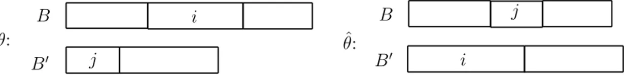
Given a production schedule, a delivery schedule θ is a partition of the orders into b batches, along with the specification of a transportation mode and the departure time for each batch.

A production-distribution schedule is specified by a production schedule σ and a delivery schedule θ. We indicate a production-distribution schedule by the pair (σ, θ). Given a production-distribution schedule, we let B(j) denote the batch of order j. The delivery time of an order j is therefore denoted by DB(j).

In all scenarios, the objective of the 3PL provider is to minimize the transportation cost T C = h1n1 + h2n2, where n1 and n2 are the number of batches of type 1

(regular) and type 2 (express), respectively. If only one transportation mode is present, the objective is to minimize the number of batches. The objective of the manufacturer is to minimize the makespan Cmax = maxj=1,...,nCj2. The values

of makespan Cmax and transportation costs T C associated with the

production-distribution schedule (σ, θ) are denoted as Cmax(σ, θ) and T C(σ, θ) respectively.

Scenarios In this chapter we consider two scenarios: (1) manufacturer dominates, 3PL provider adjusts; (2) 3PL provider dominates, manufacturer adjusts. These are formally defined in the following.

(40)

1. Manufacturer dominates, 3PL provider adjusts - scenario 1.

(a) Manufacturer’s problem. The manufacturer determines an optimal pro-duction schedule in two steps. In the first step, because of the dominance, the manufacturer can plan his schedule disregarding the role of the 3PL provider, i.e., assuming that each order will be transported to M2

imme-diately after release from M1. Hence, in the first step, the manufacturer

faces a 2-machine permutation flow shop scheduling problem with a con-stant transportation time-lag. Following the three-field notation α|β|γ for machine scheduling problems (Graham et al. 1979), this problem is denoted by F 2|time − lag|Cmax. In the second step, the manufacturer first imposes

the constraints, i.e. the release time C1

j and the deadline dj of order j,

j = 1, . . . , n, to the 3PL provider. Then, the manufacturer adjusts the start-ing time of the orders on M2 on minimizing Cmaxsubject to the delivery times

Dj of each order j = 1, . . . , n offered by the 3PL provider and the sequence

of production on M1.

(b) 3PL provider’s problem. Given the release time C1

j and the deadline dj of

each order j, j = 1, . . . , n, the 3PL provider aims at finding a delivery sched-ule that minimizes the transportation cost T C and such that each order is delivered to M2 within dj, i.e., it must hold Dj ≤ Cj1+ T . The 3PL provider’s

problem can be seen as an IPODS (Integrated production and outbound dis-tribution scheduling) problem with a single machine, deadlines and direct batch delivery to a single customer, in which the sequence on the machine is fixed. Following the five-field notation α|β|π|δ|γ of Chen (2010), the problem can therefore be denoted as 1|f seq, dj = Cj1+ T |π|1|T C, where:

α: 1 refers to a single machine (M1) and fseq indicates that the sequence on

M1 is fixed,

β: deadlines are defined as C1 j + T ,

π: this field may contain the following values: direct indicate the direct batch delivery V1_(x

(41)

reg-3.2. Problems and Notations 31

ular transportation (either limited or unlimited) and y1 ∈ {c1, ∞} is

the capacity of each vehicle for regular transportation (either limited or unlimited).

V2_(x

2, y2), where x2 ∈ {V2, ∞} represents the total number of

ve-hicles for express transportation (either limited or unlimited) and y2 ∈ {c2, ∞} represents the capacity of each vehicle for express

trans-portation(either limited or unlimited).

δ: this field is equal to 1, which refers to a single customer (M2)

γ: this field contains the objective function, which is the total cost to the 3PL provider (T C).

2. 3PL provider dominates, Manufacturer adjusts - scenario 2.

(a) 3PL provider’s problem. In this scenario, on the one hand the 3PL provider wants to relax the responsiveness by increasing the value of T , on the other hand he want to find the best constraints of release time by imposing the delivery schedule to the manufacturer. With the necessary information of production, i.e. the processing time of orders on M1, the 3PL provider aims

at determining a production-distribution schedule (hence, both a production schedule on M1 and a delivery schedule) such that the transportation cost

T C is minimized, while delivering each order within T from its release by M1

(i.e., dj = Cj1 + T for each order j). We consider production schedules in

which M1 continuously processes orders, with no idle time. This constraint

enforces a minimum productivity requirement. This problem can be seen as an IPODS problem, denoted by 1|no−idle, dj = Cj1+T |π|1|T C. In the β field

we specify that M1 must never be idle, while π is as described in the previous

scenario. Then according to the obtained schedule, the 3PL provider offers a limited set of regular vehicles and express vehicles with given capacities and transportation times to the manufacturer.

(b) Manufacturer’s problem. The manufacturer determines a production schedule on both machines minimizing the Cmax subject to a limited set of

Coordination d'ordonnancement de production et de distribution

Universit´e Paris-Dauphine

´

Ecole doctorale de Dauphine

Th`

ese

Pour l’obtention du grade de

Docteur en informatique

Coordination of production and

distribution scheduling

Coordination d’ordonnancement de production et de

distribution

Pr´esent´ee par : Liangliang FU

Soutenue le 2 d´

ecembre 2014 devant le jury compos´

e de :

Directeur de th`

ese :

Rapporteurs :

Examinateurs :

Abstract

R´

esum´

e

Acknowledgements

Contents

I

Production and Interstage Distribution Scheduling

23

II

Production and Outbound Distribution Scheduling

93

List of Figures

List of Tables

Chapter 1

Introduction

1.1

Background

1.2

Contribution

1.3

Organization of the dissertation

Chapter 2

Literature Review

2.1

Production scheduling

2.2

Distribution scheduling

2.3

Integrated production and distribution

schedul-ing

2.4

Supply chain scheduling

Part I

Production and Interstage

Distribution Scheduling

Chapter 3

Individual Production and

Interstage Distribution Scheduling

Problems

3.1

Introduction

3.2

Problems and Notations