an author's https://oatao.univ-toulouse.fr/27143
Aguirre, Miguel Angel and Duplaa, Sébastien Epsilon: An Open Source Tool for Exergy-Based Aerodynamic Analysis. (2020) In: Aerospace Europe conference 2020, 25 February 2020 - 28 February 2020 (Bordeaux, France).
AEC2020_466
Epsilon: An Open Source Tool for Exergy-Based Aerodynamic Analysis
Miguel Angel Aguirre(1), Sébastien Duplaa(2),(1)
ISAE-SUPAERO, Université de Toulouse (France), Email: [email protected] (2)
ISAE-SUPAERO, Université de Toulouse (France), Email: [email protected]
KEYWORDS: exergy analysis, aerodynamics,
drag bookkeeping, Paraview, CFD, wind tunnel.
ABSTRACT:
This paper presents the open source code called “Epsilon”. It is a tool suited for the aerodynamic analysis of CFD and wind tunnel data by using the exergy method. Other methods are also provided (near-field, far-field, Lamb vector). The architecture of the code is presented as well as a qualitative description of the analysis capabilities provided by the tool. Some reference test cases are presented and an accuracy assessment of the exergy analysis is performed. The software is released to the public along with this conference paper.
1. NOMENCLATURE
𝒜̇ = total rate of anergy, W 𝒜̇𝑤 = shock wave anergy, W𝒜̇𝛷 = viscous dissipation anergy, W
𝒜̇𝛻𝑇 = thermal mixing anergy, W
a = speed of sound, m.s-1 c = airfoil chord, m CD = drag coefficient
Cp, Cv = mass specific heat at constant pressure
and at constant volume, J.kg-1.K-1 D = drag force, N
dc = drag count, (1dc=0.0001 CD)
e = mass specific internal energy, J.kg-1 𝐸̇𝑢 = axial kinetic exergy, W
𝐸̇𝑣 = transverse kinetic exergy, W
𝐸̇𝑝 = boundary-pressure work rate, W
hs, ht = specific static and total enthalpy, J.kg -1
i, j ,k = unit vectors along the x-, y- and z-axes
M = Mach number (= u0/a0)
n = 𝑛𝑥 i, 𝑛𝑦 j, 𝑛𝑧 k, local surface normal
Ps, Pt = static and total pressure, Pa
Pr = Prandtl number R = gas constant, J.kg-1.K-1
Re = Reynolds number (= 𝜌0 𝑢0 c / 𝜇0)
S = surface, m2
s = mass specific entropy, J.kg-1.K-1 Ts, Tt = static and total temperature, K
V = ui, vj, wk, local velocity vector, m.s-1
= angle of attack, deg
= ( ) – ( )0, local variation of a parameter
respect to the upstream reference value 𝜀̇𝑚 = mechanical exergy, W
𝜀̇𝑡ℎ = thermal exergy, W
𝛷𝑒𝑓𝑓 = effective dissipation, W.m-3
γ = ratio of specific heats
eff = effective thermal conductivity, W.m -1
.K-1
μ, μ
t = laminar and turbulent dynamicviscosities, kg.m.s-1
= air density, kg.m-3
𝝉̿
= viscous stress tensor, Pa( )∗ = isentropic component of the variable ( )
( ) ̅̅̅ = non-isentropic component of ( ) Subscripts 0 = Upstream values b = body surface w = wake region
out = outlet plane (infinite survey plane)
2. INTRODUCTION
The aerodynamic analysis based on the exergy method is gaining interest in the research community and the industry as it provides a powerful performance assessment for any configuration, regardless its complexity [1-5]. Indeed, it became the most suited tool for the study of future aircraft configurations where complex engine/airframe interactions are present [6,7]. Nevertheless, this method is not yet used massively. One of the reasons behind is that very few exergy-based CFD posttreatment codes are available today and all of them are paid software. ISAE-SUPAERO decided to overcome this drawback by developing an open source exergy analysis tool suited for CFD and experimental data (wind tunnel testing).
3. CLASSICAL METHODS
Before presenting the exergy method, the classical aerodynamic analysis methods are reviewed. This will give a reference against which the advantages of the exergy method can be compared.
3.1. Reference system
All the formulations discussed below uses a standard reference frame as described in Fig.1. It considers a reference system where the x-axis is aligned with the upstream flow direction and pointing rearwards, the y-axis points towards the right-hand side of the body and the z-axis points upwards. The x-, y-, z-axes will be called “aerodynamic axes” (or “wind axes”). Moreover, when control volume formulations are used, it is supposed that the outlet section of the control volume is a plane (called “survey plane”) and it is placed normal to the x-axis (i.e., normal to the upstream flow direction). Also, the lateral surfaces are considered parallels to the upstream direction and far away from the body.
Figure 1. Conventional reference frame
3.2. Near-field method
The most used method for aerodynamic analysis is the near-field approach, which allows calculating drag by performing a body surface integral [8,9]:
𝐷 = ∫ (𝑃𝑆𝑏 𝑠 𝒏𝒙− 𝝉̿ . 𝒏𝒙) 𝑑𝑆𝑏 (1)
This approach has the advantage of being very simple and easy to understand. However it only decomposes the drag into its pressure and friction components, which does not give a complete understanding of the physics: this highlights its drawbacks for design analysis purposes (which becomes especially true for the analysis of complex configurations).
3.3. Far-field method
A more powerful aerodynamic assessment can be made by using the so-called far-field methods. All of them apply the momentum conservation equation to a control volume surrounding the body in order to define a set of equations thereby
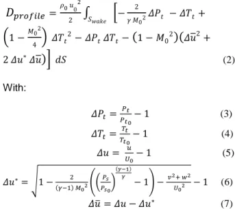
allowing a phenomenological decomposition of drag, while giving at the same time a good insight into the physics. Several variants of this method are available, [10-17] each that allow the extraction of the drag force by only analyzing the wake of a body. For simplicity, we will use here the Meheut’s method, which is suited for the wind tunnel measurement of stationary flows [17]. It is based on the small perturbations method and the decomposition of the axial velocity deficit inside the wake. This leads to the following profile drag equation which is valid for compressible and incompressible regimes:
𝐷
𝑝𝑟𝑜𝑓𝑖𝑙𝑒 =𝜌0 𝑢02 2∫
[
− 2 𝛾 𝑀02𝛥𝑃𝑡 − 𝛥𝑇𝑡+ 𝑆𝑤𝑎𝑘𝑒(
1 −𝑀02 4)
𝛥𝑇𝑡 2− 𝛥𝑃 𝑡 𝛥𝑇𝑡−(
1 − 𝑀02)(
𝛥𝑢̅
2+ 2 𝛥𝑢∗ 𝛥𝑢̅)]
𝑑𝑆 (2) With: 𝛥𝑃𝑡=𝑃𝑃𝑡 𝑡0− 1 (3) 𝛥𝑇𝑡=𝑇𝑇𝑡 𝑡0− 1 (4) 𝛥𝑢 = 𝑈𝑢 0− 1 (5) 𝛥𝑢∗= √1 − 2 (𝛾−1) 𝑀02(( 𝑃𝑠 𝑃𝑠0) (𝛾−1) 𝛾 − 1) − 𝑣2 𝑈+ 𝑤2 02 − 1 (6) 𝛥𝑢̅ = 𝛥𝑢 − 𝛥𝑢∗ (7)The “small perturbation” assumption considers that the variations of total pressure 𝛥𝑃𝑡, total
temperature 𝛥𝑇𝑡 and velocity Δu are small.
Moreover, the velocity perturbation Δu is decomposed into a viscous contribution 𝛥𝑢̅ (which is null outside the wake) and other component 𝛥𝑢∗
that is related to the isentropic field.
For 2D applications, the profile drag is the total drag acting upon a body (which includes the viscous drag and the wave drag). For 3D cases, the vortex drag must also be considered:
𝐷𝑣𝑜𝑟𝑡𝑒𝑥 = ∫𝑆𝑜𝑢𝑡𝜌2(𝑣2+ 𝑤2) 𝑑𝑆 (8)
𝐷𝑡𝑜𝑡𝑎𝑙= 𝐷𝑝𝑟𝑜𝑓𝑖𝑙𝑒+ 𝐷𝑣𝑜𝑟𝑡𝑒𝑥 (9)
Although this method provides a deep physical understanding, it is not suited for the analysis of complex systems like a strongly-coupled powered aircraft, where the thrust-drag bookkeeping is no longer possible [6]. This issue can be solved by using the exergy analysis, which provides at the same time, an even deeper physical analysis than the far-field method.
S
oU
oS
lateralS
outS
wakex
y
z
4. EXERGY ANALYSIS
Exergy is a Thermodynamic concept based on the first and second laws [18-19] as shown in Fig.2.
Figure 2. The origin of the exergy analysis
It considers the flow around a body as an energy system that can be splitted into two parts: the exergy (its useful part -it can be recovered-) and the anergy (its useless part-it is already lost-). This is depicted in Fig.3.
Figure 3. The exergy analysis principle
The energy of a system may be converted to work only if the system is not in equilibrium with its environment. It does not matter if the system represents a sink or a source of energy (low temperature for example), what matter is the imbalance itself. Thus, any disturbance of the flow field has an energy potential (more precisely, an exergy potential). An increase of air velocity inside a jet or the low speed inside the wake of a profile contains an amount of energy that can be
recovered (Fig.4). Hence, exergy represents the theoretical maximum amount of work that can be recovered by bringing the system back to thermodynamic equilibrium with its environment by following a reversible transformation.
Figure 4. Energy recovery principle
The exergy “𝜀” of a system is given by:
𝜀 = 𝛿ℎ𝑡− 𝑇𝑠0 𝛿𝑠 = 𝛿ℎ𝑡− 𝒜 (10)
There are several exergy-based formulations for aerodynamic analysis [1-7, 20-22]. Here, the Arntz’s formulation [1] will be used since it is suited for the analysis of CFD simulations and also because it is widely used for the analysis of future aircraft configurations [7]. This approach allows calculating the drag of a body from an exergy-based point of view as follows: 𝐷 ∗ 𝑢0= 𝜀̇ + 𝒜̇𝑐𝑟𝑒𝑎𝑡𝑒𝑑= 𝜀̇𝑚+ 𝜀̇𝑡ℎ+ 𝒜̇ (11)
Where the exergy (𝜀̇) was splitted into its mechanical (𝜀̇𝑚) and thermal (𝜀̇𝑡ℎ) components. The related drag coefficient is then given by: 𝐶𝐷𝜀= 𝜀̇𝑚+𝜀̇𝑡ℎ+𝒜̇ 1 2𝜌0 𝑢03 𝑆𝑟𝑒𝑓 (12) The mechanical exergy is given by the sum of the axial kinetic exergy (a quantity related to the perturbations of the axial velocity component), the transverse kinetic exergy (a quantity related to the perturbations of transverse velocity components) and the boundary-pressure work rate (a quantity related to the pressure perturbations): 𝜀̇𝑚= 𝐸̇𝑢+ 𝐸̇𝑣+ 𝐸̇𝑝 (13)
𝐸̇𝑢= ∫𝑆𝑜𝑢𝑡12𝜌 𝛿𝑢2(𝑉⃗ . 𝑛⃗ )𝑑𝑆 (14)
𝐸̇𝑣= ∫𝑆𝑜𝑢𝑡12𝜌(𝑣2+ 𝑤2) (𝑉⃗ . 𝑛⃗ ) 𝑑𝑆 (15)
𝐸̇𝑝= ∫𝑆𝑜𝑢𝑡(𝑃𝑠− 𝑃𝑠0)[(𝑉⃗ − 𝑉⃗ 0). 𝑛⃗ ]𝑑𝑆 (16)
Also, the thermal exergy represents a quantity related to the temperature perturbations:
Velocity perturbation = energy that can be recovered
ε̇th= ∫𝑆𝑜𝑢𝑡ρ δe (V⃗⃗ . n⃗ ) dS+ ∫𝑆𝑜𝑢𝑡Ps0(V⃗⃗ . n⃗ ) dS−
Ts0∫𝑆 ρ δs (V⃗⃗ . n⃗ ) dS
𝑜𝑢𝑡 (17)
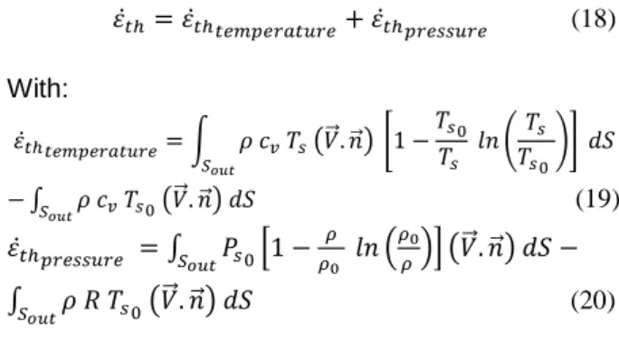
An alternative expression for 𝜀̇𝑡ℎ is given by [1, 22]:
𝜀̇𝑡ℎ= 𝜀̇𝑡ℎ𝑡𝑒𝑚𝑝𝑒𝑟𝑎𝑡𝑢𝑟𝑒+ 𝜀̇𝑡ℎ𝑝𝑟𝑒𝑠𝑠𝑢𝑟𝑒 (18) With: 𝜀̇𝑡ℎ𝑡𝑒𝑚𝑝𝑒𝑟𝑎𝑡𝑢𝑟𝑒= ∫ 𝜌 𝑐𝑣 𝑇𝑠 (𝑉⃗ . 𝑛⃗ ) [1 − 𝑇𝑠0 𝑇𝑠 𝑙𝑛 ( 𝑇𝑠 𝑇𝑠0)] 𝑑𝑆 𝑆𝑜𝑢𝑡 − ∫𝑆𝑜𝑢𝑡𝜌 𝑐𝑣 𝑇𝑠0 (𝑉⃗ . 𝑛⃗ ) 𝑑𝑆 (19) 𝜀̇𝑡ℎ𝑝𝑟𝑒𝑠𝑠𝑢𝑟𝑒 = ∫ 𝑃𝑠0[1 −𝜌𝜌 0 𝑙𝑛 ( 𝜌0 𝜌 )] (𝑉⃗ . 𝑛⃗ ) 𝑑𝑆 𝑆𝑜𝑢𝑡 − ∫𝑆 𝜌 𝑅 𝑇𝑠0 (𝑉⃗ . 𝑛⃗ ) 𝑑𝑆 𝑜𝑢𝑡 (20)
Finally, the anergy represents the amount of exergy that has been actually destroyed as a result of irreversibilities (entropy generation by viscous dissipation, shockwaves and thermal gradients):
𝒜̇ = 𝑇𝑠0∫𝑆 𝜌 𝛿𝑠 (𝑉⃗ . 𝑛⃗ ) 𝑑𝑆
𝑜𝑢𝑡 (21)
The total anergy can then be decomposed into its viscous, thermal and wave components as follows:
𝒜̇ = 𝒜̇𝛷+ 𝒜̇𝛻𝑇+ 𝒜̇𝑤 (22) 𝒜̇𝛷= ∫ 𝑇𝑇𝑠0 𝑠 𝑣 𝛷𝑒𝑓𝑓 𝑑𝑣 (23) 𝒜̇𝛻𝑇= ∫ 𝑇𝑇𝑠0 𝑠2 𝑣 𝑘𝑒𝑓𝑓 (𝛻𝑇)2 𝑑𝑣 (24) 𝒜̇𝑤= 𝑇𝑠0∫𝑆𝑤𝑎𝑣𝑒(𝜌 𝛿𝑠 𝑉⃗ ). 𝑛⃗ 𝑑𝑆 (25) With: 𝜅𝑒𝑓𝑓 = 𝑐𝑝((𝑃𝑟𝜇) + (𝑃𝑟𝜇𝑡 𝑡)) (26) 𝛷𝑒𝑓𝑓= (𝜏 ̿. 𝛻). 𝑉⃗ (27)
The interest of the exergy method is that it provides a powerful insight into the physics: if a
survey plane is placed just downstream of a body there is certain exergy available (related to the velocity, pressure and temperature perturbations) as well as certain amount of anergy (related to the losses occurred upstream, inside the boundary layer and wake). As the survey plane moves downstream, viscous and thermal dissipation takes place, which reduces the available exergy. This exergy destruction process is equal to the amount of anergy created (i.e., proportional to the entropy generation). Finally, if the survey plane is placed at an infinite distance downstream, all the exergy that was available at the trailing edge of the body has now been destroyed: there is only anergy left. Moreover, at any plane position, the sum of exergy and anergy gives the drag coefficient (Eq.12). In particular, when the survey plane is placed far downstream, drag is only given by anergy (i.e., given by the total entropy generation [12]).
5. EPSILON
Epsilon is an open source aerodynamic analysis tool suited for CFD and experimental data. It allows the user to perform an aerodynamic analysis by using the exergy method as well as the classical methods (near field, far-field and Lamb vector).
Epsilon is a set of plugins for Paraview created to provide an easy to use tool for the post processing of 2D and 3D data as shown in Fig.5. The code was developed at ISAE for research purposes (Development of new exergy formulations [20-22]) and now is released to the public along with this conference paper under GNU GPL V3 license. It can be downloaded from this internet site:
https://Epsilon-Exergy.isae-supaero.fr The site also contains plenty of related information: user manual, tutorials, open data as well as some theory.
5.1. Capabilities
Since Epsilon was conceived as an aerodynamic analysis tool, it includes the classical aerodynamic parameters used for performance assessment (like total pressure loss). On the top of that, the main four aerodynamic analysis methods are provided: near-field, far-field, Lamb vector and Exergy. Some of the parameters available in the code are the following (non-exhaustive list):
a) Classical aerodynamic analysis:
• Pressure coefficient (Cp)
• Total pressure ratio (Pt/Pt0)
• Vortex detector (Q criterion, Lambda 2) [23] • Shock wave detection (Fig. 6) [24]
b) Near-field method [8-9] c) Far-field methods: • Momentum conservation [9] • Betz [10] • Jones [11] • Oswatitsch [12] • Maskell [13]
• Van Der Vooren [14] • Giles [15] • Kusunose [16] • Meheut [17] d) Lamb-vector method • Wu [25] • Marongiu [26] e) Exergy method • Arntz [1] • Aguirre [20-23]
Moreover, since Epsilon is a flexible platform, it also allows the user to implement new equations or variables by simply modifying a Python code.
Figure 6. Shockwave detection in CFD example
5.2. Architecture
Epsilon is basically a set of plugins for Paraview. Paraview has been selected as a platform because it is open source, user-friendly and widely used by the CFD community [27]. The plugins allows Paraview to execute several Python files that calculates the aerodynamic parameters.
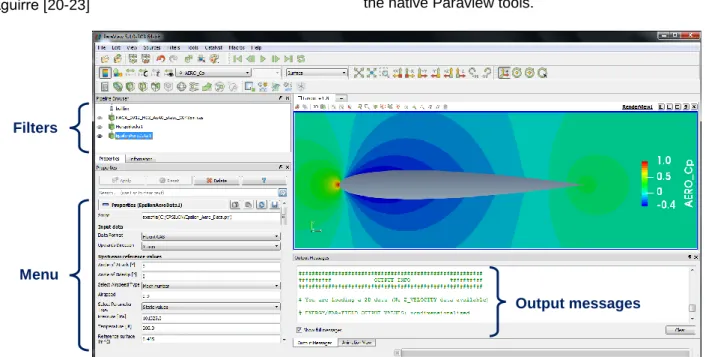
The user simply has to load its CFD/experimental data into Paraview and to execute Epsilon Aero Data (The main Epsilon plugin). Then, he is ready to perform an aerodynamic analysis as depicted in Fig.7 and 8.
Epsilon Aero Data provides all the variables associated to the methods indicated in Section 5.1 which can be easily visualized and integrated with the native Paraview tools.
Figure 7. Interface of Paraview/Epsilon
Output messages Filters
Figure 8. Architecture of Epsilon
In some cases, the user may want to perform deeper analyses that require using tools not available in Paraview by default. That is why Epsilon provides some ready-to-use analysis tools (e.g., automatic integration methods).
5.3. Analysis tools
The most typical aerodynamic analysis is to plot the distribution of a certain parameter along the chord or span of a body, as shown qualitatively in Fig. 9 for the spanwise lift distribution
Figure 9. Example of lift distribution
Since lift, drag and exergy are integral quantities, this kind of plot requires first performing a plane integral at several stations and then to plot the integrated values along the desired axis. This is achieved by the automatic integration tool provided by Epsilon. In order to do that, a survey plane is created and the desired positions of the plane are defined as shown in Fig. 10 for a 3D case (the same applies for a 2D case). Then, the tool performs an automatic integration at each position and hence the output can be plotted along the sweeping direction as shown qualitatively in Fig. 11.
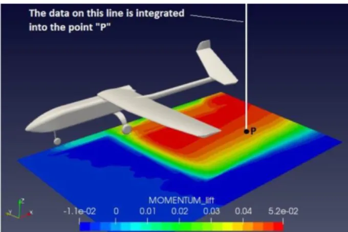
On the other hand, the same integration concept can be further extended for the case of 3D data. In
those cases a line can be used instead of a plane for the integral. This allows the integration of the 3D volume data into a plane as shown in Fig. 12, where each point of the plane represents the local integral of the 3D domain in a direction normal to the plane. This kind of mapping is very useful for the analysis of complex configurations.
Figure 10. Survey plane and plane positions
Figure 11. Axial distribution of profile drag
Figure 12. Integration of 3D data into a plane
Another tool provided by Epsilon is a Poisson equation solver. This tool is required for the Maskell method in order to calculate the induced drag. This tool solves the Poisson equation starting from the axial vorticity field and gives the related stream function as shown qualitatively in Fig. 13.
CFD/experimental DATA
Epsilon Aero Data
Data visualization and integration
Automatic Integration methods
Figure 13. Stream function in the survey plane
5.4. Data formats
Several commercial CFD solvers are supported by Epsilon by default. CFD data from other solvers can be easily read by writing a small Python script. Moreover, experimental data can also be analyzed with Epsilon: PIV (2D2C, stereo and 3D) as well as directional probes (five-hole probe and seven-hole probe). An example of this is shown in Fig. 14 (PIV data by courtesy of Y. Bury). The gray region is the PIV measurement area and the black line represents the contour of the body.
Figure 14. Axial exergy field from the stereo PIV wake measurement of an aircraft afterbody [28]
5.5. Future developments
Epsilon was originally intended for the analysis of external aerodynamic cases. However, since the code is under continuous development, new features will be available soon.
The software has been tested on steady-state adiabatic unpowered external aerodynamic cases. Future work intends to extend its capabilities to cover unsteady flow, heat transfer and powered cases (e.g., aircraft engine integration). Also, turbomachinery applications are no currently explicitly supported but this will be available soon (still under development). However, it is reminded that Epsilon is a flexible platform allowing the user to easily implement his own equations.
6. TEST CASES
6.1. Geometries
In order to verify the accuracy of the software for the prediction of the drag coefficient, 2D and 3D CFD data was used: a NACA 0012 airfoil with sharp trailing edge and a rectangular wing with the same airfoil and aspect ratio 8. The CFD data presented hereafter is available in the website. Hence, the results shown in this paper can be reproduced by the users.
6.2. Mesh
Although any kind of mesh can be used in Epsilon, the wake analysis methods (far-field, Lamb vector and exergy) require some specific requirements. As a matter of fact, most of CFD meshing techniques only refine the region close to the wall (Boundary layer mesh) but not inside the wake. However, this kind of mesh is not suited for the wake analysis methods as a large numerical dissipation will take place inside the wake region due to the lack of cell refinement. Hence, a suited mesh must have a proper wake refinement in order to ensure that the losses are convected downstream from the body to the survey plane position without numerical dissipation.
A mesh that satisfies this requirement is shown in Fig.15 and 16, where the wake refinement region is shifted for different angles of attack in order to properly capture the wake. It is a C-type multiblock structured mesh created in ICEM CFD with 593.000 cells. The boundaries of the domain are placed at ±150 chords from the airfoil to minimize the interaction of the body with the boundaries as shown in Fig. 17 .For the 3D case, the boundaries are placed at ±30 chords and the mesh contains 9.196.000 cells (Fig.18). In all cases, Y+ value is less than 1 at any surface point.
Figure 16. C-grid structured mesh suited for α=10°
Figure 17. mesh of the entire domain (α=0°)
Figure 18. Surface mesh for the 3D case (α=0°)
6.3. Solver setup
RANS simulations were run with ANSYS Fluent 16.2 solver. Reynolds number was fixed at 3.0x10⁶ and the Mach number was varied from 0.3 to 0.8. In all cases, Spalart Allmaras turbulence model was used, along with Roe flux type and density
based solver. A first quick convergence was made with a first-order discretization (flow and turbulence) by about 3000 iterations, followed by a final 2nd order interpolation scheme for flow and turbulence (Fig.19). All the simulations were left running until the near-field drag coefficient residual was less than 0.1dc (drag counts). At the same time, the residuals must reach their maximum precision in order to ensure that the airfoil’s losses were completely convected downstream. Then, the y+ parameter was controlled in order to verify that y+≤1 everywhere around the body (as required by the Spalart Allmaras model).
Figure 19. Residuals convergence for the airfoil at α=0°/M=0.3
6.4. Grid convergence
In order to verify the accuracy of the CFD solution, a grid convergence study was made by using three grid levels: coarse, medium and fine (Table 1).
Mesh
size Coarse Medium Fine
Extra-fine
Cells
count 145.000 593.000 2.187.000 8.065.715
Table 1. Airfoil mesh sizes
The Richardson extrapolation technique [29] was used to obtain a higher-order extrapolated values (corresponding to an extra-fine mesh). The resulting near-field drag coefficient (extracted from the solver FLUENT) was compared in Fig.20 against experimental data with transition fixed at the leading edge [30] (because SA turbulence model does not predict boundary layer transition). The medium mesh was retained for all cases.
Figure 20. Grid convergence for α=0°/M=0.3
7. VALIDATION
The comparison of the near-field drag values from Fluent against experimental data just provides an assessment of the quality of the simulation itself but it does not provide an assessment of the performance of Epsilon. Since Epsilon is a posttreatment software, the only way to assess its performance is by comparting the near-field drag values from Fluent to the far-field and exergy-based drag values from Epsilon. If a good agreement between near-field and far-field/exergy values is found, it means that:
• The mesh is properly refined along the wake. • The posttreatment provided by Epsilon is good.
7.1. Drag coefficient comparison
Far-field and exergy drag coefficient values are extracted by using a survey line as shown in Fig.21 for the 2D case (For the far-field method, the survey line only covers the wake region).
Figure 21. Survey line and field of exergy-based drag density for M=0.3 and α=10°
Table 2 shows the far-field and exergy drag values extracted with Epsilon at 1 chord downstream of the airfoil. These values are compared against the near-field drag coefficient extracted from Fluent. A very good agreement is observed as expected, because those methods are supposed to analyze the same physics from different points of view.
M / α [°] Near-field Far-field Exergy
0.3/0° 91.5 91.68 91.75 0.75/0° 86.39 86.18 86.47 0.8/0° 158.7 158.7 158.94 0.3/10° 153.55 149.82 152.5 0.75/3° 302.19 301.69 302.27 0.8/2.5° 388.11 387.8 388.34
Table 2. Profile drag coefficient [drag counts] for the 2D airfoil (survey plane 1 chord downstream)
The differences among these methods are related to several reasons. On one hand, there are the assumptions required for each method. In this regard, the Meheut’s far-field method is the most compromised as it relies on the small perturbations theory (whose effect is noticeable in the case M=0.3/α=10°, where it shows a difference of almost 4dc respect the near-field value). On the other hand, there are numerical issues playing a major role, like the wake refinement discussed before.
A way to assess the quality of the wake refinement is by sweeping the survey plane position downstream of the body and by comparing the drag coefficients at all positions. This is shown in Fig. 22 for the M=0.3/α=0° case, where the x-axis has the origin at the leading edge, hence x/C=1 is the trailing edge position. A very good correlation is observed for all the methods at any plane position, even at large distances from the body.
Figure 22. Profile drag at several survey plane positions (M=0.3 and α=0°)
The drop of the predicted drag coefficient for the Meheut’s method when the survey plane is very close to the body is a typical drawback of the far-field methods [21], which is not present in the exergy method.
For the 3D case the data is integrated on a survey plane as shown in Fig. 23. Drag values are shown in Table 3 where a good correlation is observed.
Figure 23. Total anergy at survey plane and shockwave volume for M=0.75/α=3°
M / α[°] Near-field Far-field Exergy
0.3/0° 94.52 94.31 95.38 0.75/0° 93.26 93.47 94.13 0.8/0° 135.72 137.1 136.79 0.3/10° 420.4 431.98 422.14 0.75/3° 209.92 211.57 211.13 0.8/2.5° 288 287.31 289.95
Table 3. Wing’s total drag coefficient [drag counts] (survey plane at 1 chord downstream)
7.2. Exergy breakdown comparison
A deeper verification of the posttreatment from Epsilon is proposed by comparing our results against reference data of the bibliography [1]. The same test case (2D airfoil at M=0.3/α=0°) will be used to compare the Fluent/Epsilon results against the elsA/ffx results (taken here as the reference value). The related distribution of exergy and anergy components downstream of the airfoil are plotted in Fig. 24 and 25 respectively. A very good correlation is observed.
Figure 24. Exergy distribution (airfoil M=0.3/α=0°)
Figure 25. Anergy distributions (airfoil M=0.3/α=0°)
Table 4 shows the actual values of these components for a survey plane placed at one chord downstream of the airfoil. The small differences found can be attributed to the fact that the CFD data is not the exactly the same (there are always small differences among different solvers even if the same mesh is used).
Data 𝜀̇𝑚 𝜀̇𝑡ℎ 𝒜̇𝛻𝑇 𝒜̇𝛷 𝒜̇ 𝐶𝐷
elsA
ffx 4.1 0.17 1.06 84.95 86.01 90.28 Fluent
Epsilon 4.08 0.17 1.25 85.48 87.5 91.75
Table 4. exergy parameters [drag counts] at M=0.3/α=0°, survey plane at 1 chord downstream
8. CONCLUSIONS
An open-source posttreatment tool for exergy analysis of CFD and wind tunnel data is released to the public domain. It has the intention of promoting the utilization of the exergy method by academics, research and industry sectors. The main target is to provide to the aerodynamicists a powerful analysis tool for performance assessment suited for any domain: aeronautics, automotive, defense and so forth.
9. ACKNOWLEDGEMENT
The authors would like to acknowledge ISAE for supporting the development of the code.
10. REFERENCES
[1] Arntz, A., “Civil Aircraft Aero-thermo-propulsive Performance Assessment by an Exergy Analysis of High-fidelity CFD-RANS Flow Solutions,” Fluids mechanics, Université de Lille 1, 2014.
[2] Drela, M., “Power Balance in Aerodynamic Flows,” AIAA journal Vol. 47, No. 7, 2009.
[3] Aguirre, Duplaa, “Exergetic Drag Characteristic Curves,” AIAA Journal, Vol. 57, No. 7, 2019. [4] Camberos, J. and Moorhouse, D., “Exergy Analysis and Design Optimization for Aerospace Vehicles and Systems,” Progress in Astronautics and Aeronautics, AIAA, 2011.
[5] Hayes, Lone, Whidborne, Camberos, Coetzee, “Adopting Exergy Analysis for use in Aerospace,” Progress in Aerospace Sciences, Vol. 93, 2017.
[6] Hall, D., “Boundary Layer Ingestion Propulsion: Benefit, Challenges and Opportunities,” 5th UTIAS International Workshop, Canada, 2016.
[7] Wiart, L. and Negulescu, C., “Exploration of the Airbus “Nautilius” Engine Integration Concept,” 31st
ICAS, September 9-14, Brazil, 2018.
[8] Drela, M., Flight Vehicle Aerodynamics, The MIT Press, Cambridge, MA, 2014
[9] Anderson, J., Fundamentals of Aerodynamics, McGraw-Hill Education, Boston, 2010.
[10] Betz, “A Method for the Direct Determination of Wing-Section Drag”, NACA TR 337, 1925. [11] Jones, “Measurement of Profile Drag by the Pitot-Traverse Method,” ARC R&M 1688, 1936. [12] Oswatitsch, K., Gas Dynamics, Academic Press Inc., New-York, 1956.
[13] Maskell, E., “Progress Towards a Method of Measurement of the Components of the Drag of a Wing of Finite Span”, RAE TR 72232, 1973. [14] Van der Vooren, “On drag and lift analysis of transport aircraft from wind tunnel measurements”, Aerospace Science and Technology 12, 2008.
[15]Giles, "Wake Integration for Three-Dimensional Flowfield Computations Theoretical Development", Journal of Aircraft, Vol 36 No 2, 1999.
[15] Giles,"Wake Integration for Three-Dimensional Flowfield Computations Theoretical Development", Journal of Aircraft, Vol 36 No 2, 1999.
[16] Kusunose, Crowder “Extension of Wake-Survey Analysis Method to Cover Compressible Flows,” Journal of Aircraft, Vol. 39, No. 6, 2002. [17] Meheut, M., “Evaluation des Composantes Phénoménologiques de la Trainée d'un Avion à
Partir des Résultats Expérimentaux,” Thèse ONERA-Université de Lille, France, 2006.
[18] Cengel, Y., Boles, M., Thermodynamics: An Engineering Approach, Eighth edition, Mc Graw Hill Education, New York, 2015.
[19]Bejan,Advanced Engineering Thermodynamics , 2nd Ed., John Wiley and Sons, New York, 1997.
[20] Aguirre, Duplaa, Carbonneau, “Vortex Exergy Prediction”, 54th 3AF Int. Conference on Applied Aerodynamics, 25 – 27 March, France, 2019. [21] Aguirre, Duplaa, Carbonneau, Turnbull, “A Systematic Analysis of the Mechanical Exergy of an Airfoil by Using Potential Flow, Euler & RANS”, 24ème CFM, France, 2019.
[22] Aguirre, Duplaa, Carbonneau, Turnbull, Arntz, “A Better Assessment of the Recoverable Energy Behind a Body by the Exergy Method”, Aerospace Europe Conference, 25-28 February, France, 2020
[23] Jeong, Hussain, “On the identification of a vortex,” J. Fluid Mech., vol. 285, pp. 69-94, 1995. [24] Lovely, D., Haimes, R., “Shock Detection From CFD Results,” AIAA 99-3285, 1999.
[25] Wu, J.M., Ondrusek, B, Wu, J.Z., “Exact force diagnostics of vehicles based on wake-plane data,” AIAA 34th Aerospace Sciences, Reno, 1996.
[26] Marongiu, Tognaccini, Ueno, “Lift and Lift-Induced Drag Computation by Lamb Vector Integration,” AIAA Journal, Vol. 51, No. 6 2013. [27] Ahrens, J., Geveci, B., Law, C., “ParaView: An End-User Tool for Large Data Visualization,” Visualization Handbook, Elsevier, 2005.
[28] Bury,Y., Jardin,T, and Klöckner, A., “Experimental investigation of the vortical activity in the close wake of a simplified military transport aircraft,” Experiments in Fluids, 54. 2013.
[29] Richardson, L. , ‘The approximate arithmetical solution by finite differences of physical problems involving differential equations, with an application to the stresses in a masonry dam’, Philosophical Transactions of the Royal Society A. 210.1911.
[30] W. McCroskey, “A Critical Assessment of Wind Tunnel Results for the NACA 0012 Airfoil,” NACA TM 100019, 1987.