Estimation de l'équivalent en eau de la neige par l'utilisation d'un système d'assimilation de température de brillance dans un modèle de métamorphisme de neige multicouche

Département de Géomatique Appliquée

Faculté des lettres et sciences humaines

Université de Sherbrooke

Estimation de l’équivalent en eau de ]a neige par l’utilisation

d’un système

d’assimilation de température de brillance dans un modèle

de

métamorphisme de neige multicouche.

Estimation ofsnow water equivalent using a radiance assïmilatîon

scheme

with a multi-layered snow physical model

AJJy MOUNIROU TOURÉ

Thèse présentée pour l’obtention du grade de Philosophiae Doctor(Ph.D.) en télédétection

Août 2009

© Ally MOUNIROU TOURÉ, 2009

Composition du jury

Cette thèse a été évaluée par un jury composé des

personnes suivantes:

Pr. Kalïfa

Goïta,

Directeur de recherche

(Département de Géomatique Appliquée, Faculté des lettres

et sciences humaines)

Pr. Christian Mitz1er, Codirecteur de recherche

(Institute ofApplied Physics, Universïty of Bern.)

Pr. Alain Royer, Codirecteur de recherche

(Département de Géomatique Appliquée, Faculté des lettres et sciences humaines)

Pr. Ramata Magagi, Examinatrice interne

(Département de Géomatique Appliquée, Faculté des lettres et sciences humaines)

Pr Norman T. O’Neill, Examinateur interne

(Département de Géomatique Appliquée, Faculté des lettres et sciences humaines)

Dr. Clins Derksen, examinateur Externe

(Climate Research Division, Environment Canada)

Présidente: Madame Thérèse Audet

(Département de psychologie, Faculté des lettres et sciences humaines)

Financial support

• This work was supported by the National Science and Engineering Research Council of Canada and by Environrnent Canada (CRYSYS Program).

I dedicate this thesis to my oncle Souradjou Yacoubou who educated me during my childhood,

supported me unconditionally and encouraged me to pursue my interests. He taught me to aiways challenge myseif in other to achieve my God-given potential.

Acknowledgem ents

f irst, I would like to express my deep and sincere gratitude to my supervisor Prof.

Kalifa Goïta and co-supervisor Prof. Alain Royer for their consistent support and advice throughout the many stages ofmy PhD. It was a privilege to work and to learn from them.

I gratefully acknowledge the financial support of the National Science and Engineering Research Council of Canada (NSERC) and Environment Canada (CRYSYS Program).

My special thanks to Prof. Christian Mitzler for the opportunity to visit the Institute of Applied Physics (lA?), University of Bern; for his invaluable insights, advice, support and encouragement throughout this work. I bas been an honour and privilege to know him and work with him.

Thanks to the Institute ofApplied Physics (JAP), University of Bern, Switzerland for the invaluable logistical supportthey provided me with for the field work,

Thanks to Martin Schneebely of Institute for Snow and Avalanche Research (SLf), Davos, Switzerland for his insights and support during my field work at Weissfluhjoch, Davos.

I am grateful tothe Centre de Calcul Scientifique (CCS) of Université de Sherbrooke and especially to HuiZhong Lu who has been helpful in programming and optimizing ofmy codes. It was wonderflil to work with him.

I am ver)’ grateflul for Dr. M. Durand of Byrd Polar Research Center, Ohio State University for his keen insights and bis valuable advice in the implementation of the data assimilation system.

I would like to thank the Centre d’Étude de la Neige (CEN) in france for providing us with CROCUS.

Thanks to my dear friend Hatiétou Camara and Gwen Jones for is unflagging support and encouragement for these 5 years.

Thanks to my family who have been a long lasting source of energy during this exhaustive research. my wonderful parents, brothers and sisters (Kande, Madina, Baba, Amine, Audu and Todje

_),

my oncles Souradjou, and Bawa, my fiance Sara and my cousin

Yahya.

Résumé

Nous avons étudié la faisabilité de l’assimilation de la temperature de brillance (Tb) pour l’estimation des paramètres physiques de la neige en utilisant un modèle de métamorphisme de neige plus réaliste que celui qui a été utilisé dans les études précédentes. Le travail se divise en cinq parties. Les deux premiers chapitres sont consacrés à la revue de la littérature.

Dans le chapitre 3 nous avons étudié l’utilisation de la photographie numérique proche-infrarouge pour estimer la longueur de corrélation de la neige pour la modélisation de l’émission micro-onde. L’étude est basée sur les travaux expérimentaux que nous avons réalisés en Avril 2006 sur la neige dans les alpes suisses. Des mesures radiométriques et proche infrarouge d’échantillons de neige sous différentes conditions expérimentales ont été réalisées. Nous avons utilisé une relation empirique pour relier la réflectance dans le proche infrarouge de la neige à la surface spécifique de la neige puis avons converti la surface spécifique en longueur de correlation.

À

partir des mesures de Tb de la neige à 21 et 35 GHz, nous avons dérivé les coefficients de diffusions micro-onde de la neige en inversant les modèles de transfert radiatif Sandwich et Six-flux. Les longueurs de corrélations que nous avons trouvées sont dans la game déterminée par des travaux antérieurs en chambre froide.

Dans le chapitre 4, la performance du filtre de Kalman d’ensemble de Monte Carlo (EnKF) pour l’estimation de l’équivalent en eau de la neige a été évaluée en assimilant les Tb simulées par un modèle physique de neige multicouche (CROCUS). Le système d’assimilation était tourné en utilisant un ensemble de 20 réplicats de données météorologiques artificiellement biaisées. Le EnKf était en mesure d’estimer la valeur de l’équivalent en eau de la neige avec une moyenne saisonnière de RMSE de 1.2 cm (8.1%). Le système était aussi capable de simuler le profil de taille de grains de neige du manteau ce qui était impossible à faire avec les systèmes d’assimilation anciens.

Dans le chapitre 5 nous avons testé le système d’assimilation avec des données in situ du CLPX-l (Cold Land Processes field Experiment-1 2002-2003). Avant de tester le système d’assimilation, nous avons d’abord procédé à la vérification de la précision de la prédiction des

Tb en couplant le modèle de métamorphisme CROCUS au modèle démission MEMLS. Nous avons trouvé que la prédiction des Tbs se comparent favorablement avec les données in situ seulement lorsque CROCUS±MEMLS est forcé avec les données météo corrigées. La précision de la prediction de Tb est entre + _{7 K et} + 40 K. La différence de polarisation est sousestimée de 25 à 75%. Nous avons enfin assimilé les Tbs mesurées dans le modèle CROCUS afin d’estimer le SWE. Le système était en mesure d’estimer le SWE avec un bias de 0.14cm et une RMSE de 1.32cm (8.3%), ce qui représente une amélioration plus de 75% sur

la valeur du RMSE lorsque CROCUS est tourné seul, sans assimilation.

Mots-clés:

Temperature de brillance, assimilation des données, equivalent en eau de la neige, modèle de métamorphisme, modèle de transfert radiatif, filtre de Kalman d’ensemble, profondeur de neige, longueur de corrélation, surface spécifique de la neige

Abstract

The feasibility ofa radiance assimilation using a multi-layered snow physical model to estimate snow physical parameters is studied. The work is divided in five parts. The first two

chapters are dedicated to the literature review. In the third chapter, experimental work was conducted in the alpine snow to estimate snow correlation (for microwave emission modelling) using near-infrared digital photography. We made microwave radiometric and near-infrared reflectance measurements of snow slabs under different experimental conditions. We used an empirical relation to link near-infrared reflectance of snow to the specific surface area (SSA), and converted the SSA into the correlation length. From the measurements of snow radiances at 21 and 35 GHz, we derived the microwave scattering coefficient by inverting two coupled radiative transfer models (RTM) (the sandwich and six-flux model). The correlation lengths found are in the same range as those determined in the literature using cold laboratory work. The technique shows great potential in the determination of the snow correlation length under field conditions.

In the fourth chapter, the performance ofthe ensemble Kalman filter (EnKf) for snow water equivalent (SWE) estimation is assessed b)’ assimilating synthetic microwave observations at Ground Based Microwave Radiometer (GBMR-7) frequencies (18.7, 23.8, 36.5. 89 vertical and horizontal polarization) into a snow physics model, CROCUS. CROCUS has a realistic stratigraphic and ice layer modelling scheme. This work builds on previous methods that used snow physics model with limited number of layers. Data assimilation methods require accurate pred jetions of the brightness temperature (Tb) emitted by the snowpack. It has been shown that the accuracy of RTMs is sensitive to the stratigraphic representation ofthe snowpack. However, as the stratigraphic fidelity increases, the number of layers increases, as does the number of state variables estimated in the assimilation. One goal ofthe present study is to investigate whether passive microwave measurements can be used in a radiance assimilation (RA) scheme to characterize a more realistic stratigraphy. The EnKF run was performed with an ensemble size of 20 using artificially biased meteorological forcing data. The snow model was given biased precipitation to represent systematic errors introduced in modelling, yet the EnKF was stili able to recover the “true” value of SWE with a seasonally-integrated RMSE ofonly 1.2 cm (8.1%). The RA was also able to extract the grain size profile at much higher dimensionality which shows that the many-to-one problem of

SWE-Tb relationship can be overcome by assimilation, even when the grain size profile varies constantly with depth.

The last chapter was on the validation of the data assimilation system using a point

scale radiance observations from the CLPX-l GBMR-7. We first predicted snow radiance by

coupling the snow model CROCUS to the snow emission model (MEMLS). Significant improvement of Tb simulation was achieved for the fate february window for ail three frequencies. The range of the underestimation of the polarization difference is between 25% and 75%. We then assimilated ail six channels measurements ofthe GBMR-7. The filter was able to accurateiy retrïeve the SWE for periods of time when the Tb measurements were available. The resuits show that RA using EnKF with a multi-layered snow mode! can be used to determine snow physica! parameters even with a biased precipitation forcing.

Keywords:

Brightness temperature, radiance assimilation, snow depth, snow water equivalent, snow physical mode!, radiative transfer model, ensemble Kalman filter, corre!ation length, snow specific surface.

Sommaire

La couverture nivale saisonnière avec sa grande variabilité temporelle a un impact important sur le climat, les processus hydrologiques et sur les activités humaines (Singh et Singh, 2001).

À

l’échelle globale, la neige influence fortement les échanges énergétiques entre la surface de la terre et l’atmosphère (Hillard et al., 2003). Sur le plan régional, elle peut être considérée comme une précieuse ressource “renouvelable”. Dans les prairies canadiennes par exemple, la neige saisonnière génère à elle seule jusqu’à 80% de l’écoulement annuel de surface (Granger et Gray, 1 990). Dans les régions à couverture nivale saisonnière, la quantité d’eau stockée dans le manteau nival, c’est-à-dire son équivalent en eau (SWE), constitue le paramètre le plus important dans l’estimation du rendement du drainage de l’eau dans le bassin versant. La connaissance des variations saisonnières de SWE est donc cruciale pour la gestion efficace des ressources en eau. Elle aide au suivi du climat, à l’amélioration des prévisions météorologiques, à la gestion et de l’approvisionnement en eau pour l’irrigation et pour les centrales hydro-électriques. Elle permet aussi d’anticiper les effets des inondations, de prédire le rendement des récoltes et de contrôler le ruissellement (Matzler, 1985).

Traditionnellement, le SWE s’obtient à partir des mesures au sol dans des sites pré-sélectionnés. Souvent, seule la profondeur de la neige est déterminée, à partir de laquelle le SWE est estimé. Ces mesures ponctuelles restent limitées dans l’espace, longues et cofiteuses. Pour une surveillance à grande échelle, les capteurs satellitaires constituent une source possible de données de la neige. Les rayonnements micro-onde, du fait de leur capacité à traverser les nuages et à pénétrer le manteau nival, constituent potentiellement un excellent moyen de détermination des paramètres physiques de la neige (étendue, profondeur, SWE) (Kunzi et al., 1982; Chang et al., 1982).

Jusqu’à une date récente, les données micro-ondes satellitaires ont été utilisées dans des algorithmes simples et directs pour estimer de manière approximative les paramètres physiques de la neige. Des régressions linéaires sont trouvées entre la température de brillance (Tb) de neige et son équivalent en eau (Chang et al., 1987; Foster et aI, 1991; Hallikainen et Jolma 1992; Goïta et al., 2003). Dans ces algorithmes, seule une fraction de l’information disponible du capteur est utilisée (par exemple seulement 2 canaux sur 9 des capteurs SSM/1 sont utilisés). Ainsi, une quantité importante d’informations est perdue. De plus, la plupart des

modèles sont très dépendants des conditions locales de la neige. Appliqués à d’autres régions de morphologie de neige et de couverture du sol différentes, leur performance se détériore rapidement (foster et al., 2005; Dong et al., 2005).

Toute l’histoire du manteau nival est stockée dans la neige par son état métamorphique. Se servir de cette information peut réduire les ambiguïtés dans l’inversion de la Tb pour l’obtention des propriétés de la neige (Mtzler, 2003). Il existe des modèles de métamorphisme de neige qui (forcés par des données météorologiques) sont capables de simuler l’évolution des paramètres physiques de la neige en fonction du temps (par exemples: CROCUS (Brun et al., 1992), SNTHERM (Jordan, 1991) et SNOWPACK (Lehning et al. 2000a, b). Aussi, il existe des modèles d’émission micro-onde de neige (exemple de MEMLS (Wiesmann et Mitzler, 1 999) capables de simuler la Tb d’un manteau de neige multicouche. Par conséquent, il est possible de simuler l’émission micro-onde du manteau au capteur si son état géophysique est connu. Au lieu d’inverser le modèle d’émission micro-onde, il peut être intégré dans un système d’assimilation de données.

L’assimilation de données est une méthode d’intégration des données satellitaires dans un modèle de métamorphisme de neige. C’est une manière implicite et plus attrayante d’inversion des modèles de transfert radiatif (Durand et Margulis, 2006). Pour que cette approche, réussisse, des modèles assez réalistes et précis de métamorphisme de neige et de transfert radiatif sont nécessaires. La determination du SWE par l’utilisation d’un système d’assimilation de Tbs a été appliquée pour la première fois par Durand et Margulis (2006). Mais dans le but de réduire la complexité algorithmique de leur modèle d’assimilation, ils ont utilisé un modèle de métamorphisme, le SAST (Simple Snow—Atmosphere—Soil Transfer model, Sun et al., 1 999) qui limite le nombre de couches de neige à trois. Ils ont conclu quafin que la Tb simulée à partir du couplage des modèles de neige et d’émission soit adéquate pour l’assimilation, le modèle de métamorphisme doit prédire de manière précise la stratigraphie des couches de neige. Ce qui signifie que le nombre de couche de neige au cours de la saison peu dépasser trois.

Le but principal de la thèse est d’étudier la faisabilité de l’assimilation de la Tb dans un modèle multi-couche de neige pour l’estimation des paramètres physiques de la neige en utilisant un modèle de métamorphisme de neige plus réaliste que celui qui a été utilisé dans les études précédentes. La question scientifique à laquelle nous avons voulu répondre est la

suivante: Est ce qu’un système d’assimilation de Tb avec le filtre d’ensemble de Kalman utilisant un modèle de métamorphisme de neige multicouche peut permettre d’estimer les paramètres physiques de la neige? Cette thèse est divisée en cinq chapitres:

Dans le chapitre 1, nous rappelons les propriétés physiques de la neige. Ces propriétés influencent la Tb de la neige. Il s’agit principalement de : la densité, la teneur en eau liquide, la taille de grains de neige et l’équivalent en eau de la neige, produit de la densité par la hauteur. Nous y discutons aussi les différents types de métamorphismes de neige, les échanges d’énergie dans la neige, ainsi que les formules utilisées pour calculer la constante diélectrique de la neige.

Le chapitre 2 traite des propriétés de diffusion micro-onde de la neige. La diffusion des micro-ondes par les grains de neige est le phénomène le plus important qui influence la Tb du manteau nival. Nous avons présenté les aspects théoriques de la diffusion et l’équation de transfert radiatif. Par ailleurs les solutions de cette équation sont aussi discutées.

Dans le chapitre 3 nous avons étudié l’utilisation de la photographie numérique proche-infrarouge pour estimer la longueur de corrélation de la neige pour la modélisation de l’émission micro-onde. Le modèle d’émission micro-onde pour les manteaux de neige stratifiés (MEMLS) est un modèle de transfert radiatif qui nécessite entre autres paramètres, la longueur de corrélation pour chaque couche de neige. La longueur de corrélation est le paramètre de structure qui est le plus critique pour le calcul de la diffusion micro-onde, et est reliée à la surface spécifique de la matrice glace-air. Des études antérieures ont démontré un fait important : pour que l’assimilation des données aboutisse à des résultats précis, le modèle d’émission de la neige doit être capable de prédire la Tb avec une précision de+ 5 K et pour que cette precision soit atteinte, le modèle d’émission de neige doit prédire la Ingueur de correlation avec une précision de +/-O.016 mm. Pour obtenir une telle précision, il est nécessaire de trouver une manière de représenter la taille de grains des modèles physiques de neige et d’émission par un même paramètre: la longueur de correlation. Pour cela, nous avons consacré le chapitre 3 à l’établissement d’une nouvelle méthode pratique de determination de la longueur de corrélation de la neige en utilisant sa surface spécifique estimée à partir de la photographie dans le proche infrarouge (NTR). La méthode traditionnelle de détermination de la longueur de corrélation exige un travail en chambre froide, long et laborieux. Ce paramètre

important d’entrée du modèle a donc été toujours impossible à mesurer directement sur le terrain. Pour contourner la difficulté de mesure de la longueur de corrélation, certains chercheurs mesurent la taille des grains de neige sur le terrain pour ensuite la convertir en longueur de corrélation en utilisant des formules empiriques. La conversion surestime souvent la taille optique des grains de neige parce que la neige est un milieu tridimensionnel et par conséquent ne peut pas être caractérisée par la taille de grains qui est un paramètre unidimensionnel. L’étude de la détermination de la longueur de correlation par la photographie NIR est basée sur les travaux expérimentaux que nous avons réalisés en Avril 2006 sur la neige dans les alpes suisses. Nous avons réalisé des mesures radiométriques et proche infrarouge d’échantillons de neige sous différentes conditions expérimentales. Nous avons utilisé une relation empirique pour relier la réflectance dans le proche infrarouge de la neige à la surface spécifique de la neige (Matzl and Schneebeli, 2006) puis avons converti la surface spécifique en longueur de correlation.

À

partir des mesures de Tbs de la neige à 21 et 35 GHz, nous avons dérivé les coefficients de diffusions micro-onde de la neige en inversant les modèles de transfert radiatif Sandwich et Six-flux (Wiesmann et al., 199$). Les longueurs de corrélations que nous avons trouvées sont dans la game déterminée par des travaux antérieurs en chambre froide.

Dans le Chapitre 4 nous avons évalué la performance du système d’assimilation de données que nous avons établi en combinant un modèle de métamorphisme de neige multicouche (CROCUS) avec un modèle d’émission de neige (MEMLS). Traditionnellement, dans l’inversion des données de télédétection micro-onde passive, des paramètres d’entrée du modèle sont traités comme résultats recherchés, lorsqu’ils permettent de minimiser (via un algorithme d’optimisation), la fonction de coût contenant la différence entre la Tb simulée par le modèle d’émission et celle mesurée par le satellite. La difficulté de cette méthode d’inversion est liée au fait que plusieurs combinaisons différentes de paramètres de neige peuvent donner une même Tb. D’où l’importance d’avoir de l’information a priori sur le manteau de neige. La Tb mesurée par les radiomètres constitue une information instantanée sur la neige. Cette mesure est souvent entachée de bruits (erreurs). Il existe des modèles de métamorphisme de neige qui, forcés par des données météorologiques sont capables de prédire les changements de la structure interne de la neige en fonction du temps. La précision de cette prédiction dépend de la qualité des données météorologiques et des approximations utilisées

pour établir le modèle. Les avantages des données satellitaires et ceux du modèle de métamorphisme peuvent être combinés en utilisant la technique d’assimilation de données: Le modèle de métamorphisme simule l’évolution du manteau nival en fonction du temps, jusqu’au moment où les mesures radiométriques soient disponibles. Les Tb mesurées, sont alors comparées à celles simulées grace au couplage modèle de métamorphisme! modèle d’émission; et quand cela est nécessaire, les résultats de la simulation sont ajustés en utilisant un algorithme d’optimisation (le filtre de Kalman d’ensemble de Monte Carlo (EnKf)). Le système d’assimilation de données se compose de trois principales parties: (1) le modèle de métamorphisme de la neige qui prédit l’évolution des paramètres physiques de la neige, (2) le modèle de transfert radiatif, qui convertit les profils de neige simulés en Tb correspondante ; et (3) l’algorithme d’optimisation, le filtre de Kalman d’ensemble (EnKF) qui corrige (ajuste) le profil simulé de neige en tenant compte des erreurs des modèles et de celles des mesures.

La performance du EnKf pour l’estimation de l’équivalent en eau de la neige a été évaluée en assimilant les Tb micro-ondes simulées par un modèle physique de neige multicouche. Les fréquences (18.7, 23.8, 36.5, 89 polarization verticale et horizontale) correspondent à celles du radiomètre «Ground Based Microwave Radiometer (GBMR-7)». Le système d’assimilation était tourné en utilisant un ensemble de 20 réplicats de données météorologiques artificiellement biaisées. Le modèle de neige a reçu des précipitations biaisées, et malgré cela l’EnKF était en mesure d’estimer ta valeur de l’équivalent en eau de la neige avec une moyenne saisonnière de RMSE de 1.2 cm (8.1%) malgré la présence d’eau liquide dans la neige en fin de saison. Le système était aussi capable de simuler le profil de taille de grains de neige du manteau ce qui était impossible à faire avec les systèmes d’assimilation anciens.

Dans le chapitre 5 nous avons testé le système d’assimilation avec des données in situ du CLPX-1(Cold Land Processes Field Experiment-1 2002-2003). Avant de tester le système d’assimilation, nous avons d’abord procédé à la vérification de la précision de la prédiction des Tb en couplant le modèle de neige (CROCUS) et le modèle d’émission de la neige (MEMLS). En considérant que les précipitations mesurées par les pluviomètres sont souvent biaisées, nous avons tourné CROCUS avec des précipitations mesurées et des précipitations corrigées. Nous avons démontré que lorsque CROCUS était tourné avec des précipitations corrigées (en multipliant la précipitation mesurée par 1 .65), la simulation de l’équivalent en eau de la neige

s’améliorait considérablement. Le RMSE de simulation de l’équivalent en eau de la neige était de 9.2% comparée à 41.6% quand CROCUS est tourné avec des précipitations non corrigées. CROCUS est ensuite couplé au modèle d’émission de la neige MEMLS, afin de prédire l’évolution saisonnière des Tbs. Les Tbs simulées par le couple CROCUS+MEMLS sont comparées aux données de vérité terrain mesurées par le radiomètres GBMR-7 lors de la campagne de terrain CLPX-l. Nous avons trouvé que la prédiction des Tbs se compare favorablement avec les données in situ seulement lorsque le couple CROCUS+MEMLS est forcé avec les données météorologiques corrigées. La précision de la prediction de Tb est entre

+ _{7 K et} ± _{40 K. La différence de polarisation est sousestimée de 25 à 75%, et cela est dû au}

fait que CROCUS simule mal la densité des couches de glace et autre couches minces qui se forment dans le manteau. L’évolution saisonnière des Tbs peut être divisée en trois parties: la première période est caractérisée par une diminution de Tbs (en fonction du temps) due à la diffusion micro-onde de la neige. La seconde période est caractérisée par des températures plus ou moins stables avec des pics dûs à l’alternance d’absorption des micro-ondes pendant le jour et de diffusion due aux couches de glace qui se forment pendant le gel dans la nuit. La troisième période est dominée par des Tbs élevées due à l’augmentation de l’absorption micro onde du fait de la présence permanente de l’eau liquide dans le manteau de neige. Nous avons enfin assimilé les Tbs mesurées dans le modèle CROCUS afin d’estimer le SWE. Le système était en mesure d’estimer le SWE avec un bias de 0.14 cm et une RMSE de 1.32 cm (8.3%), ce qui représente une amélioration plus de 75% sur la valeur du RMSE lorsque CROCUS est tourné seul, sans assimilation.

Table of Contents

Introduction .1

Chapter I: Physical properties ofsnow 6

1.1 Description ofsnow 6

1.1.1 Basic properties ofsnow 6

1.1.1.1 Density 7

1.1.1 .2 Grain shape and grain size 7

1.1.1.3 Liquid water content 9

1.1.1 .4 Snow Water Equivalent (SWE) 9

1.1.2 Snowmetamorphism 9

1.1 .2.1 Equi-tempçrature metamorphism j

o

1.1.2.2 Kinetic metamorphism 10

1.1.2.3 Melt+refreeze metamorphism ₁₁

1.2 Snow energy and mass balance ₁₂

1.2.1 Energy balance ₁₂

1.2.2 Mass balance ofthe snowpack ₁₃

1.3 Snow as a dielectric medium 15

1.3,1 Maxwells equations 15

1.3.2 Effective permittivity of mixture 17

1.3.3 Application to snow ₁₉

1.3.3.1 Dielectric constant ofdry snow 20

1.3.3.2 Dielectric constant ofwet snow 23

1 4 Conclusion ₂₆

Chapter II: Snow as a scattering medium ₂₇

11.1. Electromagnetism ofsnow 27

11.1.1 Scattering amplitude ₂₇

11.1 .2 Approximate scattering models 30

11.1 .2.1 Rayleigh scattering for small spheres 30

11.1 .2.2 The Born approximation 33

11.1.2.3 Semi-empirical formulae for the computation ofsnow scattering coefficient... .34

11.1.3. Absorption coefficient ₃₄

11.2 Radiative transfer 35

11.2.1 Radiance ₃₆

11.2.2 Radiation in thermal equilibrium ₃₆

11.2.3 Radiation in local thermodynamic equilibrium and Kirchhoffs law 38

11.2.4 Radiative Transfer Equation (RTE) 39

11.2.4.1 RTE for an absorbing and emitting medium 39

11.2.4.2 RTE for an absorbing, emitting and scattering medium 39

11.2.4.3 Solutions to the RTE 41

11.3 Microwave response ofsnow 43

11.3.1 Main contributions to snow microwave signature 43

11.3.2 Microwaves properties ofseasonal snow 44

11.3.2.1 Snow-free case ₄₄

11.3.2.2 Winter snow ₄₅

11.3.2.3 Spring snow ₄₅

11.3.2.4 Refrozen crust ₄₆

11.4 Conclusion ₄₇

Chapter III: Near-infrared digital photography to estimate SHOW correlation Iength for

microwave emission modelling ₄₉

111.1 Introduction ₄₉

111.2 The experiments ₅₁

111.2.1 The geographical location ofthe site ₅₁

111.2.2 Material ₅₂

111.2.3 Tb measurement procedures 53

111.2.3.1 Removal ofthe slab 54

111.2.3.2 Measurements ₅₄

111.2.4 Near infrared Photography ₅₅

111.2.5 CorreÏation ofreflectance and SSA ₅₆

111.3 Radiometric properties ofthe snow slab ₅₆

111.3.2 Brightness temperature ofthe snow on absorber .5$

111.4 Results and discussion 62

111.5 Conclusion 70

Chapter IV: Synthetic radiometric data assïmilation scheme for estimation of snow water

equivalent using the Ensemble Kalman Filter 72

1V. 1 Introduction 72

IV.2 Data assimilation system 73

IV.2.l Snow physical model (CROCUS) 74

IV.2.l.l Relationship between the CROCUS snow grain size parameters and the snow

optical diameter 76

IV.2. 1 .2 Evolution of dendricity, sphericity and size in dry snow 77

IV.2.2 Radiative transfer model (RTM) 7$

IV.2.3 Ensemble Kalman Filter $0

IV.3 Simulated experiment for veriing the assimilation scheme $2

IV.4 Resuits and discussion $5

IV.4.1 Influence ofthe ensemble size $5

IV.4.2 Snow depth $6

JV.4.3 Snow density $7

IV.4.4 Snow water equivalent 88

IV.4.5 Snow optical grain size .91

IV.4.6 Temperature 94

IV.4.7 Liquid water content 96

IV.4.$ Influence ofthe measurements errors 9$

TV.5 Conclusion 99

Chapter V: Point-scale radiometrïc data assimilation for estimation ofSHOWwater

equivalent: validation and testing 100

V.Ï Introduction 100

V.2 Validation ofthe assimilation scheme; overview 100

V.3 Experimental site and dataset 101

V.3.1 Geographical location ofthe site 101

V.3.2 Meteorological forcing: Precipitation and air temperature 105

V.4 Resuits and discussion .107

V.4.] Snow depth and SWE simulation using CROCUS 107

V.4.2 Temporal behavior oflb from CROCUS+MEMLS coupling 112

V.4.3 GBMR-7 radiance assimilation 118

V.5 Conclusion 122

Conclusion and recommendations 124

LIST 0F FIGURES

Figure 1.1.: Mechanisms of destructive metamorphism: a dendritic crystal is transformed into

rounded grain (from Canadian Avalanche Association, 199$) 10

Figure 1.2.: Mechanisms ofkinetic metamorphism: formation offaceted (multi-face) grains. The arrows show the direction ofmovement of water vapor

(http://www.enm.bris.ac.uk!teaching/projects/ 2002_03! jb83 5 5/introduction.html) 11

Figure 1.3: Constructive metamorphism: formation of depth hoar layer 11

Figure 1.4.: Melt+refreeze metamorphism: Microscopic images ofclustered rounded crystals held together by large ice-to-ice bonds (http://www.anri.barc.usda.gov/emusnow/comparison

/comp7.htm) 12

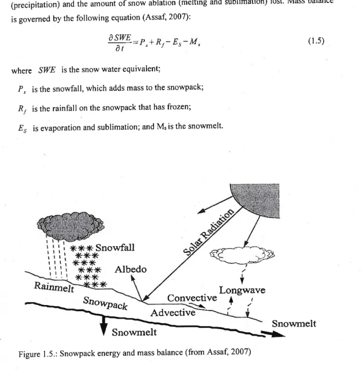
Figure 1.5.: Snowpack heat and mass balance (from Assaf, 2007) 14

Figure 1.6.: Concept ofthe effective permittivity of an heterogeneous medium: a) spherical particles are guest in a dielectric background host, and b) the effective medium that lias the same behaviour in term ofdielectric constant as the inhomogeneous medium 1$

Figure 1.7: Plots ofpermittivity of dry snow versus snow density: Mitz1ers empirical model is compared to Hallikainens and Tiuris models. The dots represent the snow dielectric

constant measured in the field by Mtzler in 1987 at Weissfluhjoch, Switzerland 21

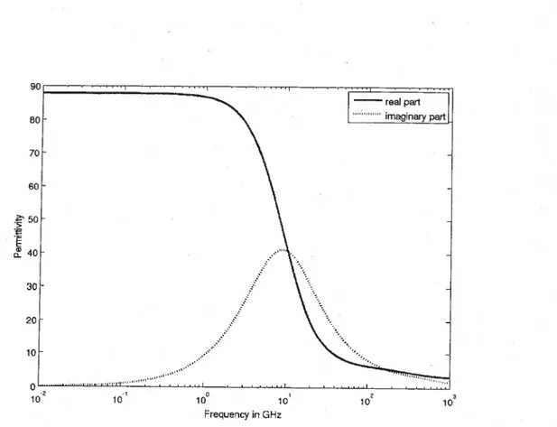
Figure 1.8.: Representation ofthe Debye relaxation equation: dielectric permittivity ofwater

at 0°C as a function offrequency (Mtzler 2005) 25

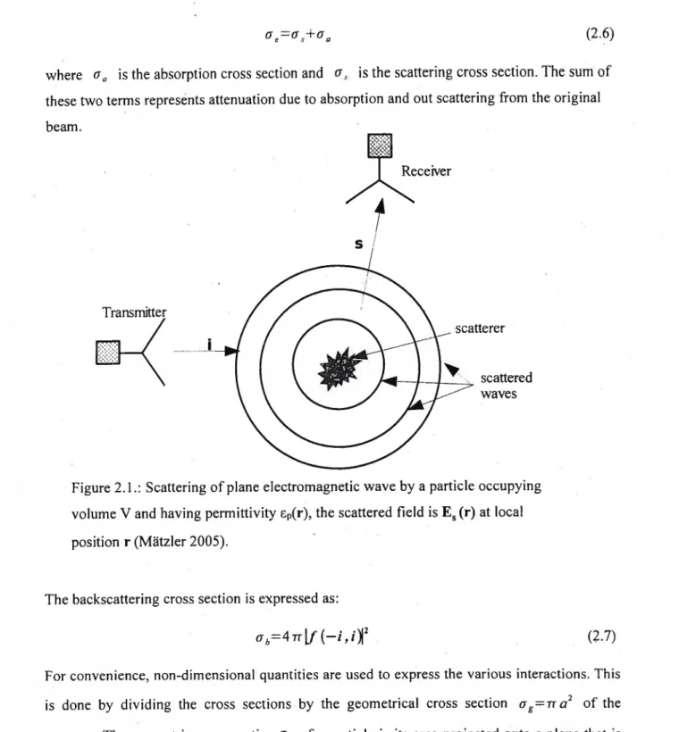
Figure 2.1.: Scattering of plane electromagnetic wave by a particle occupying volume V and having permittivity Ep(r), the scattered fleld is Es (r) at local position r (Matzler 2005) 29

Figure 2.2.: Illustration of scattering geometry; I and s are unit vectors in the direction ofthe incident and scattered waves, respectively, O is the angle between i and s, and is the angle

between E and S. (Mtzler, 1987) 31

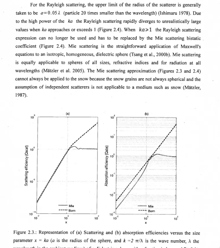
Figure 2.3.: Representation of(a) Scattering and (b) absorption efficiencies versus the size parameter x= ka (a is the radius ofthe sphere, and k =2 rr/À is the wave number, Â the

wavelength in the ambient medium) ofa dielectric sphere with refractive index m=1.7+0.lj comparison between Mie scattering and Dom approximation (Mtzler, 2005) 32

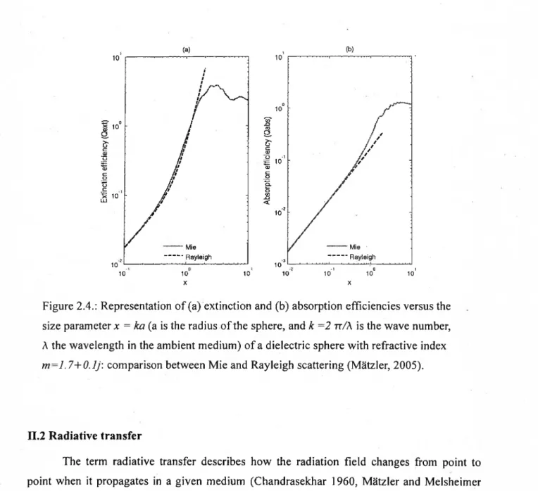
Figure 2.4.: Representation of(a) extinction and (b) absorption efficiencies versus the size parameter x = ka (a is the radius ofthe sphere, and k =2 TrIA is the wave number, À the

wavelength in the ambient medium)ofa dielectric sphere with refractive index m=1.7+0.1j:

comparison between Mie and Rayleigh scattering (Mtzler, 2005) 35

Figure 2.5.; Geometrical situation used to define the radiance: the differential solid angle dQ=sin0d8d in the spherical coordinates r, O and c; the area element dA is also shown

(modified from Tsang et al. 2000b) 3$

Figure 2.6.: A volume element dVds.dA where absorption and emission take place 39

Figure 2.7.: A volume element dV=ds.dA where absorption, emission and scattering take

place 40

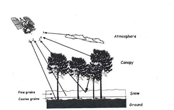
Figure 2.8.: The main contributions to the microwave emission measured by a spaceborne radiometer: (I) upward emitted soil emission contribution; (2) contribution from the snowpack (emission/scattering); (3)combined contribution from the canopy and the snowpack, (4) contributions from the forest canopy, (5) contributions from the atmosphere 43 figure 2.9: Semi-log representation ofemissivities at H and V pol. as well as their p01.

difference at 500 _{nadir versus frequency for rocky sou (lefi-hand graph) and (right-hand} graph) for dry, deep snow (without melt; SWE: 25-63 cm). The error bars show the standard

deviations from the mean emissivities (from Mitzler, 1994) 46

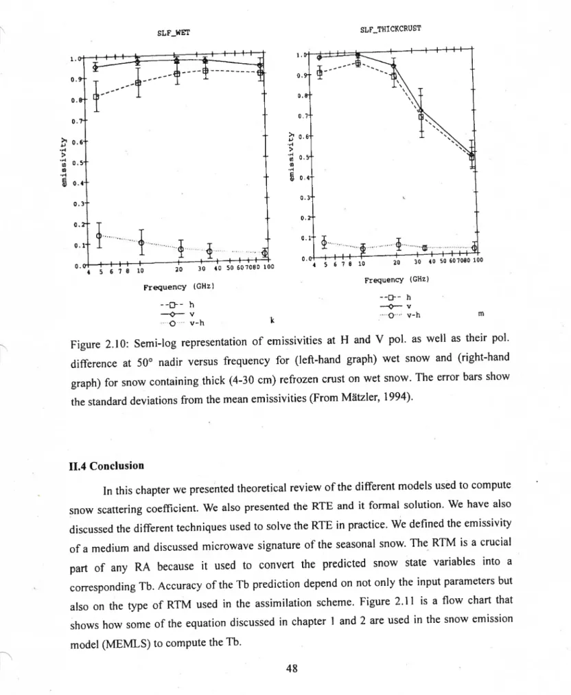
Figure 2.10.: Semi-log representation ofemissivities at H and V poi. as well as their pol. difference at 50° nadirversus frequency for (left-hand graph) wet snow and (right-hand graph) for snow containing thick (4-30 cm) refrozen crust on wet snow. The error bars show the standard deviations from the mean emissivities (From Mtz1er, 1 994) 47

Figure 2.11.: Computation ofTb using RTM model (MEMLS) 48

Figure 3.1.: Experimental setup: the radiometer is mounted on a frame directed at the snow sample (9 to 20 cm) which is placed on a 3 cm-thick styrofoam plate on a metal table

(aluminum). An absorber or metal plate is inserted between the sample and the styrofoam. The

polycorder (PC) and the battery box are also shown 53

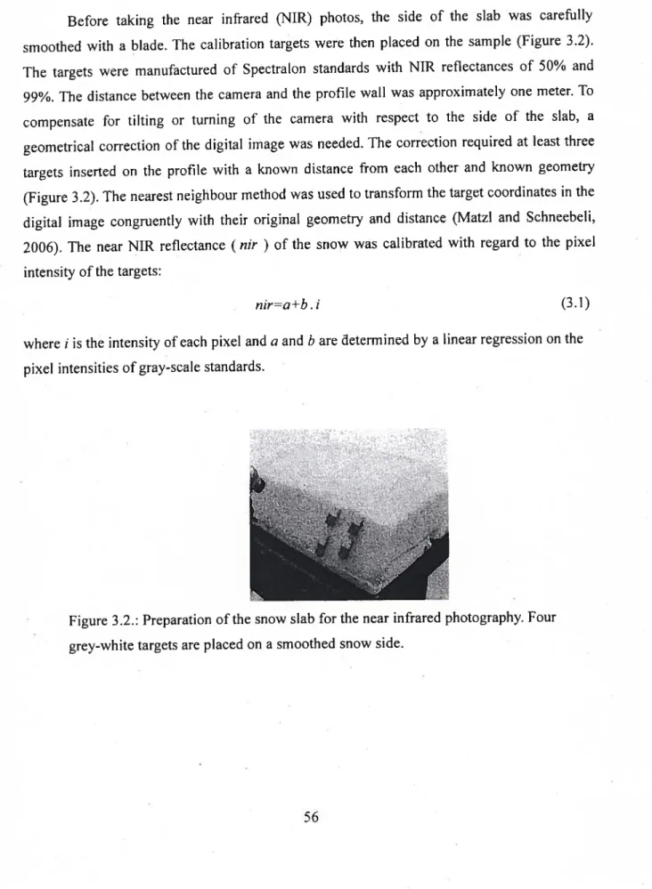
Figure 3.2.: Preparation ofthe snow slab for the near infrared photography. Four grey-white

targets are placed on a smoothed .snow side 55

Figure 3.3.: NIR photo ofa 13-cm thick inhomogeneous slab laying on a blackbody and styrofoam siabs: the top layer is a newly fallen snowwith high NIR (SSA38.5 I mm), the middte layer is a refrozen snow with very low NIR (SSA=7.7 I mm) and the bottôm layer is

made up of rounded snow (SSA=17.5 /mm) 56

Figure 3.4.: Principle of snow sample measurements: (a) measurement of brightness temperature ofsnow on metal plate, (b) measurement ofbrightness temperature ofsnow on absorber. Corresponding values ofblackbody radiation were also measured 58 Figure 3.5.: Computation of 6-flux scaflering coefficients ofthe snow samples 61 Figure 3.6.: Scatterplot ofSSA and snow mean density. Three different types of snow are

distinguished: snow with density

p<200

kg.m-3 (shown as triangles), density 200<p<300 kg.m-3 (shown as filled circles) and snow with density p>300 kg.m-3 (shown as diamonds) .63 figure 3.7.: Representation ofthe scattering coefficient at (a) 21 GHz vertical polarization, (b)

35 GHz vertical polarization, (c) 21 GHz horizontal polarization, (d) 35 GHz horizontal polarization versus the SSA. Samples with density p<200 kg.m-3 are shown as triangles. Samples with density p>200 kg.m-3 are shown in fihled circles. The numbers on the right of the symbols indicate the sample’s number. The solid une is the exponential fit ofthe dense

samples ₆₄

Figure 3.8.: Representation ofthe scattering coefficient at ta) 21 GHz vertical polarization, (b)

35 GHz vertical potarization, (c) 21 GHz horizontal polarization, (d) 35 GHz horizontal polarization versus snow density. The numbers on the right ofthe symbots indicate the

sample’s number ₆₆

Figure 3.9.: Double logarithmic representation ofthe scattering coefficients at (a) 21 GHz vertical polarization, (b) 35 GHz vertical polarization, (c) 21 GHz horizontal polarization, (U) 35 GHz horizontal polarization versus the correlation length. Samples with a density p<200 kg.m-3 are shown as triangles; samples with a densi.ty p>200 kg.m-3 are shown in filled circles. The numbers on the right ofthe symbols indicate the samples number. The solid une is the power law fit ofthe dense samples and the dash une represents power law fit found by

Wiesmann et al. (199$) _6$

Figure 3.10.: Comparison ofmeasured Tb ofsnow placed on metal plate with snow emission model (MEMLS) predictions: ta) and (b) represent the results at 21 GHz V and H polarization; (c) and (U) represent the results at 35 GHz V and H polarization _69’ Figure 4.1.: Snow radiance assimilation scheme: This illustrates how information, moUds and

radiometric measurements are merged using the EnKF ₇₄

Figure 4.2.: Representation of(a) the bias and (b) RMSE ofthe SWE estimate based on

assimilation with different numbers ofreplicates _$6

Figure 4.3.: Retrieval ofsnow depth estimate obtained by assimilating synthetic observations corresponding to GBMR-7 frequencies using the EnKf scheme. The “true” is the soiid line, the open-loop is the dotted line, faint dotted unes are individual replicates, and the EnKF

estimate (ensemble mean) is the dashed une _$8

Figure 4.4.: Retrieval of(a) snow minimum density, (b) maximum density, (c) average density. The “tnie” is represented by the solid ]ine, the open-loop is the dotted une, the faint dotted unes are individual replicates, and the dashed line is the EnKf estimate (ensemble mean). The “truth’. the open-loop and the EnKF estimate are ail superimposed in ta) 90 Figure 4.5.: Retrieval of SWE. The “truth” is the solid une, the open-loop is the dotted line, faint dotted unes are individual replicates, and the EnKF estimate (ensemble mean) is the

dashed une ₉₁

figure 4.6.: Retrieval ofthe mean optical grain size The “truth” is the solid une, the open

loop is the dotted une and the EnKf estimate (ensemble mean) is the dashed une 92

Figure 4.7.: Retrieved optical grain size profiles on 2/02/2003 93

Figure 4.8.: Retrieved optical grain size profiles on 25/03/2003 94

Figure 4.9.: Snow temperature predicted by EnKf: (a) the minimum temperature and (b) the maximum temperature. On ta), the open-loop and the filter estimate are superposed and on (b),

the truth is superposed on the estimate 95

Figure 4.10.: Retrieved Liquid Water Content (LWC in g.cm-3) ofthe snowpack. (a) minimum LWC for the snowpack, (b) maximum LWC for the snowpack and (c) weighted

mean density ofLWC for ail layers ofthe snowpack 97

Figure 5.1.: Nested study areas for the Cold Land Processes field Experiment. The map limits describe the Large Regional Study Area (4.5 x 3.5 degrees) in north central Colorado and south central Wyoming (outer square). The Small Regional Study Area (2.5 x 1 .5 degrees) boundaries are also shown. Within that area are the three 25-km x 25-km study areas: North Park, Rabbit Ears, and Fraser. Each ofthese three areas contains four l-km x 1-km Intensive Study Areas (flot shown).(From http://www.nohrsc.nws.gov/cline/clpx.html) 102 Figure 5.2.: Layout ofthe l-ha Local Scale Observation Site (LSOS) (located in the Fraser area) for Intensive Observation Periods (10?) 3 and 4 (february and March, 2003) (Graft et al.

2003) ₁₀₃

Figure 5.3.: Overview ofthe observation site: detail ofthe “open area” shown in Figure5.2, including the area observed by the GBMR-7. The oyais show the location of ail scan fields

observed by the GBMR-7 (From Graf et ai., 2003) 104

Figure 5.4.: Evolution of daily air temperature and precipitation measured at the LSOS site during 2002-2003; zero degree Celsius is indicated with a dashed horizontal line 107 Figure 5.5.: Evolution of(a) snow depth, (b) SWE simulated by CROCUS. forced with

meteorological data from the LSOS (Fraser area, Colorado,USA) 111

figure 5.6.: Measured compared to modelled Tbs (18.7 GHz and 550

incidence angle). “corrected” and ‘biased” refer to CROCUS±MEMLS runs using corrected and biased

precipitation values ₁₁₂

Figure 5.7.: Measured compared to modelled Tbs (36.5 GHz and 55° incidence angle). “corrected” and biased refer to CROCUS+MEMLS fun using corrected and biased

precipitation values ₁₁₄

“corrected” and biascd refer to CROCUS+MEMLS run using corrected and biased

precipitation values 116

Figure 5.9.: Snow wetness (w) profiles collected at snow pits #3 (Mardi 26, 28 and 30, 2003) and #4 March(25, 27. and 29, 2003) (From Tedesco et al., 2006c) 117 Figure 5.10.: Photography ofsnow pit #4 on Match 29, 2003. The total snow depthwas 60 cm (Graf et aI., 2003). Different types ofsnow layers can be identified: the top layet is fresh snow+ two meit-refrozen ]ayers (grey color) sandwiching a rounded-grain dry ]ayer+ bottom

wet snow layer 117

Figure 5.11.: Estimates of(a) snow depth, (b) SWE obtained by assimilating measured GBMR-7 Tbs using the EnKf scherne with CROCUS+MEMLS as the modefling kernel. The vertical unes shows the update times: from I O to 13 Dec. 2002, 1 $ to 26 Feb. 2003 and on 25

Match 2003 121

Figure 5.12.: Snow optical grain size profiles sirnulated on 24/02/2003 122

LIST 0F TABLES

Table 1.1.: Density range of different forms of snow (from Singh and Singh 2001) 7 Table 1.2.: Snow grain types and their size range (from Colbeck et aI. 1990) $

Table 3.1.: Properties ofthe portable Dicke Radiometers 52

Table 3.2.: fit parameters for the six-flux scattering coefficient versus the correlation length

and the correlation coefficients (d2, c3, R) compared to those determined by Wiesmann et al.

(1998) (d2wie, c3wie, Rwie

)

67

Table 4.1.: Technical specifications ofthe Ground Based Microwave Radiometer (GBMR-7)

(Graf et al., 2003) 85

Table 4.2.: The seasonal average bias and RMSE ofthe snow depth estimate compared with “true’ estimates. Values in parenthesis represent the ratio

(%)

ofthe RMSE divided by the

seasonal average ofthe “true’ snow depth 87

Table 4.3.: The season average bias and RMSE ofthe SWE estimate compared with the ‘true’ estimates. Values in parenthesis represent the ratio

(%)

ofthe RMSE divided by the seasonal

average ofthe “true’ SWE 89

Table 4.4.: The bias and RMSE ofthe SWE estimate for different assumed values ofthe standard deviation ofthe Tbs masurements error. Values in parenthesis are the ratio ofthe

RMSE over the seasonal mean SWE 98

Table 5.1.: Summary ofthe spatial, temporal coverage and resolution ofthe CLPX-1

meteorological, radiometric and snow pit measurements at the LSOS site, Colorado, USA..106 Table 5.2.: Results of different runs of CROCUS forced with precipitation data corrected with varying coefficients. The values in parenthesis represent the ratio of RMSE to the seasonally averaged snow depth or SWE expressed as a percentage. The computations over season

exciude the ]ast two weeks ofMarch 110

Table 5.3.: Bias and RMSE ofsnow depth and SWE estimate ftom the assimilation GBMR-7

Tb observations and the open-loop simulation. The values in parenthesis represent the ratio of

RMSE to the seasonal average snow depth or SWE (expressed as a percentage). The averaging period is limited to those days which were bracketed by the Dec. 10-13 and feb. 18-26 Tb

LIST 0F SYMBOLS

f

: Inclusion fractional

Ice fraction,

Pice t Ice density in kg / m3 t Permittivity ofthe inclusions

Ee : Permittivity of the host environment.

Eeff t Effective perm ittivity ofa heterogeneous material

T : Temperature in Kelvin

y Frequency in GHz

V0 t Relaxation frequency in GHz

cr, t Absorption cross section.

Scattering cross section. Optical grain size in mm SSA : Snow specific area

pc t Correlation length

Maximum diameter of snow grain, a Albedo ofthe snow surface.

Ed permittivity of dry snow

t Real part of factor of diy snow

Imaginary part if dry snow Density of dry snow in kg / m3 À Wavelength

White noise

Introduction

The seasonal snow cover lias a very strong impact on climate, hydrological processes and on human activities (Kukla, 1981). It may cover at its maximum extent as much as 62% of the Eurasian continent and ai] ofAmerica north of 35 degrees (Singli and Singli, 2001). The role ofthe snow cover may be considered in various scales. On the large scale, the seasonal snow is a critical variable in the global climate system (Kukla and Robinson, 1981). Snow cover, because of its high aibedo and latent heat, modifies energy exchanges between the surface and atmosphere (Walsh et al. 1982; Derksen and LeDrew, 2000). As the frozen storage term in water balance, snow is considered, on the regional scale as a valuable resource. Monitoring of the snows extent, water equivalent and melting condition is essential for hydrologicat forecasts in many regions, providing basic data for hydroelectric power generation, fresh water supply, river traffic, irrigation and flood control. With the increasing world populations ever increasing demand for fresh water, the optimum management of this resource is becoming important. The total amount of water stored in a snowpack is an important parameter for hydrological and water management applications. Knowing the snow water equivalent (SWE), and its distribution helps to follow the development oftheclimate, to improve weather forecasts, to predict water supply for irrigation and hydro-power stations, to anticipate flooding and to forecast crop yields (Mitzler. 1987).

Traditionally, SWE is obtained from ground measurements at selected sites. for.dry

winter snow, often only the snow depth is determined, from which the water equiva]ent can then be estimated. These spot measurements are spatially limited, time consuming and costiy. For large-scale monitoring, satellite sensors are the optimum sources ofsnow data. Visible and near-infrared satellite remote sensing provides coverage of snow extent at a reiatively high resolution and accordingly valuable data for hydrology (Rango, 1983). The shortcomings of these data sources are the frequent cloudiness in many regions of the world, the underestimation of the cover where dense forests mask the underlying snow and the lack of information on the snow depth (Kukia and Robinson, 1981; Dewey and Heim, 1981). Microwave remote sensing lias great potential because of the capabilities for depth penetration, all-weather observation and night-time viewing. Due to its ability to penetrate the snowpack and the frequency-dependent scattering losses in diy snow, spaceborne microwave measurements can be used for an effective monitoring of snowpack parameters (area extent,

depth, water equivalent, wet/dry state) (Kunzi et al., 1982; Chang et al., 1982).

Until recently, two different approaches were used to estimate SWE using microwave measurements. The first approach is purely empirical. Linear regression relationships are found between the snow brightness temperature (Tb) and its water equivalent (Chang et al., 1987: foster et al., 1991: Hallikainen and Jolma, 1992; Goïta et al. 2003). These sorts of algorithms are generally based on correlation between ground-based and satellite-borne measurements. Most ofthem are tuned to regional snow conditions. If applied to regions with different snow morpliology and land cover, the performance deteriorates drastically (Foster et al., 2005; Dong et al., 2005). Errors between 25 and 60% have been reported for some regression formulas (Foster et al. 2005). Also, the estimates tend to saturate for moderately deep snow depth (50 to 100 cm) (Chang et al., 1982; Chang et al., 1987). This makes them unsuitable for use in areas where the snow depth exceeds a meter.

The second approach is a direct inversion of a radiative transfer moUd (RTM). The technique uses measured Tb and a RTM, to determine estimates ofthe model parameters given the best fit with the observations (Menke, 1984). This is the analytical approach. f irst, the snow emission is modelled with realistic snow parameters

(

depth, density, liquid water content, correlation length (grain size). What is simulated here is the interaction of electromagnetic waves with elements that the snow is composed of: air, ice, and liquid water (when snow is wet) (Matzler, 1 987). The forward modelling leads to a deeper physical understanding of the interaction of electromagnetic waves with the snow cover. Examples of such physically-based RTMs are: Dense Media Radiative Transfer (DMRT; Tsang et al., 2000a) and the Microwaves Emission Model ofLayered Snowpack (MEMLS; Wiesmann and Matzler, 1 999). Whcn the input parameters are available, these moUds can accurately predict the Tb ofthe snow cover (Andreadis et al., 2007). The inversion is performed by considering as retrieved quantities, those parameters that minimize a cost function containing the difference between radiative transfer model predictions and measured values of the Tb observation through an optimization algorithrn (Qin et al., 2006). Direct inversion of RTM to retrieve SWE is difficult mainly because of the many-to-one nature of the SWE-Tb relationship (Durand and Margulis, 2006), and also because of the uncertainties in the forward modelling and noise in the data. The direct inversion is often ill-posed becausethere are only a few measurement channels and a large number ofunknown state variables.

To address the problem ofthe many-to-one nature ofthe SWE-Tb relationship, Armstrong 2

et al. (1993) proposed the use of apriori knowledge for ensuring the stability ofthe inversion process and reducing uncertainties in retrieved resuits. Tait (1998) used o priori

meteorological and geographic data to ciassify pixels and performed separate regressions on each. In the process of inverting the Helsinki University ofTechno!ogy snow emission mode! (RUT, Pulliainen et al., 1999), snow grain size is given a certain weight and added to a cost function as one constraint for yie]ding the maximum likelihood estimate for SWE. Josberger and Mognard (2002) developed an airground temperature gradient estimate of grain size, and integrated it into an SSMJI snow depth algorithm. Sturm and Benson (1997) developed a time dependent estimate of grain size and KelIy et al. (2003) integrated it into an AMSR-E snow depth algorithm. f oster et ai. (2005) pointed out that most errors are due to inaccurate grain diameter information and vegetation and proposed adjustments for the Chang et al. (1987) algorithm for each of these factors. Even though these algorithms incorporate a priori information, they do not estimate the uncertainty in the inversion (Foster et al. 2005). Uncertainty estimation can be thought of as obtaining thesecond moment of distribution ofthe quantity of interest, given the measurements (Qin et al., 2006). More genera]ly, a posterior distribution of the quantity of interest, inclusive of ail moments of the probability density function, is sought. It is significant to get the posterior distribution of the quantity of interest. First, it benefits the quantitative assessment of uncertainties in retrieval parameters. Second, the poster ior distribution could be treated as a priori knowledge for the next inversion (Qin et al., 2006).

Data assimilation is a scheme to merge observations with modelled data (Evensen, 1994; Rami!J and Snyder, 2000; Houtekamer and Mitcheil, 1998; Keppenne, 2000; Mitchell and Houtekamer, 2000; Anderson, 2001; Bishop et al., 2001; van Leeuwen, 2001; Reichie et al., 2002; Whitaker and Rami!!, 2002; Tippett et al., 2003; Ott et al., 2004). This approach is an implicit and more attractive way of inverting the RTMs (Durand and Margulis, 2006). Tb assimilation (RA) using Ensemble Kaiman filter (EnKF), a recursive fiiter suitable for problems with a large number of variables (Evensen, 1994), is a promising way to retrieve SWE from satellite lb observations (Durand and Margulis, 2006; Durand et al., 2007). The EnKF is an attractive data assimilation option because (j) its sequential structure is convenient for processing remotely sensed measurements in real time, (ii) it provides information on the estimate accuracy, and (iii) it is ab!e to account for a wide range of possible model and measurement errors. Satellite data gives a “snapshot” ofthe snow lb (Qin et al., 2006). Many

land surface models (LSM) have the ability to predict the changes in the snowpack with time, using surface meteorological forcing. Prediction accuracy is limited because of mode! inaccuracy (imperfect parameterization of snow dynamics) and errors in the meteorological forcing. Accuracy is also limited due to the spatial variability ofthe snow cover within a pixel and, the lack of in-situ measurements for comparison, over time as well as over a significant spatial scale, when compared with passive microwave observations (foster et al. 2005). Using the EnKF capitalizes on the LSM capability to capture the snow metamorphism dynamics and also the satellite measurement capability to provide real-time information about the state ofthe system. The LSM predicts the evolution of the snowpack, until new satellite Tbs become available. At this time the new measured lb is compared to the modelled snowpack lb and the snowpack properties are corrected on the basis ofthe observations. To make this comparison, it is necessary to estimate the satellite lb using a RTM from the simulated snow profile (Graf et al., 2006).

A number of studies have applied a product-based (SWE derived from empirical formulas) assimilation methods for deriving the SWE (Siater and Clark, 2006; Andreadis and Lettenmaier, 2006). Durand and Margulis (2006) were the first to study the feasibility ofa Tb based assimilation. They used three-layer LSM (Simple Snow—Atmosphere—Soi! Transfer moUd (SASI), Sun et al. 1999) with synthetic (simuÏated) measurements to design a season long, local-scale lb RA experiment in order to test the feasibility of SWE estimation. Synthetic measurements at SSM/I and AMSR-E frequencies and synthetic broadband albedo observations were assimilated simultaneously in order to update snowpack states in a LSM using the EnKF. Because the LSM uses a limited number of snow layers (maximum of three layers), it does flot realistical]y simulate the snow stratigraphy needed to improve lb simulations. Durand et al. (200$) recently demonstrated that stratigraphic errors due to a 3-layer snow scheme could lead to errors higher than 10 K for the 19 and 37 GHz channels.

Su êt al. (2008) suggested that a mu]ti-layer approach could significantly enhance the assimilation quality mainly because it improves the observation prediction accuracy by the coupling ofthe LSM and the RIM. Durand et al. (200$) found that in order for the predicted lbs from a coupled LSM and RIM to be adequate for RA purposes, the prediction accuracy must be within +5 K. For this accuracy to be obtained, the following conditions must be met:

1) the LSM snow layering scheme must accurately simulate the stratigraphic snowpack layers.

2) the formation of ice layers due rnelt+refreeze metarnorphism must be accurately modelled

and 3) the correlation Jength, the grain size parameter used bythe Microwave Emission Model of Layered Snowpacks (MEMLS, Wiesmann et Matzler, 1999)) must be predicted within + 0.01 6 mm. The correlation Jength can be defined as a measure ofthe average distance beyond which variations of the dielectric constant in one region of space become uncorrelated with those in another region (Parwani, 2002). The correlation length is the most critical input parameter for RTM because it is use to compute the snow microwave scattering. The traditional method ofdetermining the correlation length involves cold-laboratorywork, which is time consuming and laborious (see (Brzoska et aI., 2001 and Legagneux etal., 2002). So far there is no practical way to determine this crucial parameters under tield conditions.

The main objective of the thesis is to develop a RA scheme that combines a realistic snow physical and emission models with snow Tb measurements for a better estimation of

SWE.

The specific objectives ofthis work are:

i) study the feasibility ofa RA into a multi-layer snow physical model to determine the

S WE.

ii) propose a new practical method of determining the correlation Iength using near infrared digital photography.

This thesis consists of five chapters. Chapter I is concerned with the snow’s physical properties and its interaction with electromagnetic radiation. Chapter 2 deals specifically with the scattering properties of the snow. Chapter 3 is about the determination of the correlation length using near-infrared digital photography. Chapter 4 deals with the RA scheme using the EnKf. Synthetic experiments are described and their efficiencies are assessed. In Chapter 5, we use the EnKf to assimilate the Ground Based Microwave Radiometer (GBMR-7) Tb in snow physical model and compare the retrieved depth and SWE to the in situ measurements.

Chapter I: Physïcal properties of snow

1.1 Description ofsnow

Snow crystals precipitate in a wide variety of shapes (c.g.: dendrites, needles and columns (Colbeck et al. 1990)). Once on the ground (deposition), snow crystals bond together to form the snow cover. With each snowfall, a new layer is added to the SIIOW cover. The properties of the new layer is ofien different from the older snow beneath it (Jordan et al., 200$). Each of the layers is characterized by more or less well-defined boundaries and by discontinuons physical properties such as temperature, density, grain size, shapes and wetness (Weise, 1 996). f orced by weather conditions, physical properties of each snow layer change with time (Jordan et al., 200$). Understanding of snow physical properties is essential for understanding the mass and heat fluxes in the snowpack and modelling of microwave emissions from the snowpack. A short description of these properties is presented in this chapter.

1.1.1 Basic properties ofsnow

Snow is a mixture of ice, air and water (wet snow). The ice particles bond together to produce a distinctive snow texture. The texture is the resuit of the distribution of shape, size and pores and water present in the medium (Jordan et al., 2008). Hydrologists usually classify snow by visual examination as “crystafline”, “powdery”, “granular”, “pellet” and “mixtures”. In terms of Iiquid water content, they classify it as dry or wet (Singh and Singh, 2001). During the season, continuous structural changes occur in the snow due to compaction (due to weight of the overlaying layers), changes in grain size and shape. The structural transformation is known as metamorphism of snow (Alford, 1974). The basic properties used to describe snow cover are: snow depth, density. liquid water content, grain size and stratigraphy (Colbeck et al.

1990).

1.1.1.1 Density

Density is a fundamental snow physical parameter. The density is determined by dividing a known mass ofsnow by its known volume.The units of density are g/cm3 or kg/m3. Density of snow varies with time because of the rnetamorphism (Colbeck et al. 1990). The density ranges of different type of snow are shown in Table 1.1.

Table 1.1.: Density range ofdifferent forms ofsnow (from Singh and Singh 2001).

Type ofsnow Density (kg.m3)

New snow (after falling in cairn) I O - 70

Wet new snow 100- 200

Settled snow 200- 300

Depth hoar 200 -300

Wind-packed snow 350 - 400

1.1.1.2 Grain shape and grain size

Newly formed snow often crystallizes in hexagonal (dendritic), needles and columns shapes (Colbeck et al. 1990; Lachapelle, 1992; McClung and Schaerer, 2005). When snow crystals deposit on the ground, they alter in form due to metamorphism. Thus, a snow cover may contain grains of different shapes. An international classification of grain shape is given in Colbeck et aï. (1990). Hydrologists define the size ofthe grains as the largesi dimension (maximum diameter, D,,.

)

ofthe the snow grain. Usually, it is measured in millirneters. A mass of snow will contain a distribution of grain sizes. The grain size is determined as the average greatest extension ofthe predominant snow grains. Colbeck’s classifications for snow grain size are given in Table 1 .2. Volume scattering of electrornagnetic waves of a granular medium such as snow, does flot depend on grain size as defined (Grenfeli and Warren 1999; Mtz1er 2002). Physically meaningful structural parameters that must be used to compute the scattering are the opticai grain size

(

D0

)

or the snow specific area (SSA) or the correlation iength (pc) (Stogryn, 1984; Lim et al., 1994; Mtzler, 1997 ; Mtzler, 2002). The D0 is

defined as the diameter ofa sphere with the same total surface area and the same volume and thus the same mass as the real grain (Grenfeli and Warren, 1999). The SSA of a granular medium is the ratio of the surface area of the grains divided by their total volume (Mtzler, 2002). The pc and the D0 are inversely proportional to the SSA. Contrary to D,nax which is a one dimensional parameter, the SSA and the pc are three-dimensional parameter that take into account the shape and size of the grains, as well as their arrangement and orientation in the snowpack (Mtz1er, 2002).

According to Debye et aI. (1957) and MitzIer (2002), the relation between the

pc

and the SSA is as follows:

(1 _f,ce)

pc4

(1.1)

where

f

pIp1

is the volume fraction ofthe ie

(

p

is the density ofthe snow and P1ce917 kg/m3 isthe density of ice). The relation between pc and D0 is as follows (Mitzler 2002):

Traditional methods of determining SSA involve analyzing thin sections of snow in cold lab (Brzoska et al., 2001 , Legagneux et al., 2002; Matzl and Schneebeli, 2006) which can

be time-consuming and laborious. A more practical method ofdetermination ofthe correlation length using the digital photography in the near-infra spectrum is the subject cf chapter 3.

Table 1 .2.: Snow grain types and their size range (from Colbeck et al. 1990)

Type ofsnow size (mm)

Veiy fine <0.2 fine 0.2—0.5 Medium 0.5—1.0 Coarse 1.0—2.0 Very Coarse 2.0—5.0 Extreme

>5

$

1.1.1.3 Liquid water content

Snow Jiquid water content (LWC) also known as free water content is defined as the water available in the liquid state in the snowpack (Singh and Singh 2001). The amount of LWC of the snow is expressed as a percentage or fraction by volume. When the LWC is less than 0.5 % by volume, a thin water film covers the ice grains. The percolation (flow of liquid water) starts when the LWC is in the range of 1 to 6 ¾ ofthe total volume (Atford, 1974). Due to dielectric losses (energy absorption), the present of liquid water in a snowpack significantly

influences its Tb (see chapter 5 section V.4.2.).

1.1.1.4 Snow Water Equivalent (SWE)

The most important physical snow parameter for hydrologists and climatologists is its water equivalent. SWE can be defined as the depth of water that would result if the entire snowpack was melted instantaneously (Jordan et al. 2008). Changes to the SWE resuits from snow accumulation and snow meit (Alford, 1974). The SWE measurement unit is meters of depth of liquid water. SWE is computed as the product ofdepth and density:

SWE (m) depth (m) x density ofsnow (kg/m 3)/ density ofwater (kg/m3)

(Note: I cm3 (1 millilitre) ofwater basa mass of I g or 1000 cm3 (1 litre) basa mass of 1000 grams (1 kilogram)).

1.1.2 Snow metamorphism

The term metamorphism describes the changes in snow structure due to compaction and heat and water vapor llow within the snowpack (McClung and Schaerer, 2005; Lachapelle, 1992). The type and the rate ofmetamorphism depend on the prevailing weather conditions (Alford, 1974). That explains why succeeding fresh snow layers evolve differently and why the snowpack becomes multi-layered (Jordan et al., 200$). There are three types of metamorphism occurring in seasonal snow cover: the equi-temperature metamorphism, the kinetic metamorphism and the melt+refreeze metamorphism (Colbeck et al. 1990).

1.1.2.1 Equ i-temperature metamorphism

The equi-temperature metamorphism is also known as destructive metamorphism because it tends to destroy the original shape of snowcrystals (Gray and Male, 1981). (Figure Ï.!). Most oflen, this type ofmetamorphism occurs in new dry snow when the snowpack is subjected to small temperature (<10°C/m) (Alford, 1974). The loosely packed dentritic and piate-like ice crysta]s break up, and are slowly transformed into rounded ice granules (f igure 1.1) with typical diameters ranging from 0.5 to 1 mm (Alford, 1974). This causes the snow cover to shrink while its density increases. The average density of the fines grain snow that resuits from the equi-temperature metamorphism is about 300 kg.m3 (Lachapelle, 1992).

Rounded SmaII

Snowflake Eroded _cnstal rounded

snowflake ‘ crystal

Ç

/

f igure 1.1.: Mechanisms of destructive metamorphism: a dendritic crystal is transformed into rounded grain (from Canadian Avalanche Association, 199$).

1.1.2.2 Kinetic nietarnorphism

The kinetic metamorphism, also known as temperature-gradient metamorphism or constructive metamorphism, occurs as a resuit transfer of mass in the vapour phase, due to a differences in temperature and vapour concentration within the snowpack (McClung and Schaerer, 2005). Because snow is a good insulator, during winter, when the air temperature becomes very low, this creates a large temperature gradient (>1 0°C/m) between the colder top layer, and the warmer layer overlaying the ground. The temperature-gradient promotes a transfer of water vapour from the bottom of the snowpack to the top. The process of water vapor transfer (Figure 1 .2) results in grain growth which leads to a formation of layer of large faceted crystals at the bottom of the snowpack, referred to as “depth hoar” or “sugar snow”(Alford, 1974) (Figure 1.3). In general. the highest crystal growth is found for large

temperature gradients and large spaces between crystals (McClung and Schaerer, 2005). This

is why the depth hoar most likely occurs in early winter while the snowpack is stiil thin

(Lachapelle, 1 992).

Figure 1.2: Mechanisms ofkinetic metamorphism: Formation offaceted (multi-face) ‘grains. The arrows show the direction ofmovement ofwater vapor (http://www.enm .bris.ac.uk!teaching/projects/ 2002_03!

jb$35 5/introduction.html).

Figure 1.3: Constructive metamorphism: formation ofdepth hoar layer Faceted

(multif ace)

grain

Roundd rain{

(0.5

- 1.5

mm)

Facted grains

(1.5

-

5 rnrn

Ground

1.1.2.3 Melt+refreeze metamorphism

Melt+refreeze metamorphism describes changes in snow structure caused by melt+freeze cycles or wetting caused by an event of ram (Alford, 1974). Because snow bas a porous structure, it is able to hold a considerable amount of melt-water. In the presence of liquid water, temperature gradients and their effects disappear (Armstrong, 1985). Liquid water retained in the pores can refreeze during the following cool night. Consecutive melt+refreeze cycles are a common occurrence during the early spring period (melt during day and refreezes at night) (Mitzler 1987). The melt metamorphism leads to a formation of large irregular clusters (Figure 1 .4). These clusters strongly influence the snow microwave emission (Mitzler et al. 1987).

Figure 1.4.: MeIt+refreeze metamorphism: Microscopic images ofclustered rounded crystals held together by large ice-to-ice bonds (http://www.anri.barc.usda.gov /emusnow/comparison/comp7.htm).

1.2 Snow energy and mass balance 1.2.1 Energy baJance

The metamorphism of snow occurs in direct response to changing thermodynamic conditions in the snow (Lehning et al.,2002a). These thermodynamic changes in snow are primarily the result of variations in the intensity of meteorological conditions (i.e. precipitation, air temperature, humidity, wind speed, incoming shortwave and longwave radiations), and the nature of the surface energy exchange process (Alford, 1974). Several energy fluxes contribute to the energy balance of the snowpack (Assaf, 2007): Shortwave radiation that is incident on the snowpack can be reflected, transmitted or absorbed. The

specific nature ofthis radiation (spectral radiance) is influenced by clouds, aerosols molecules

in the atmosphere and by reflection from the snowpack (figure 1.5). An important factor

influencing albedo (reflectance to incident irradiance) depends on snow optica] grain size (Dozier et aI., 1981, Nolin and Dozier, 2000). A long-wave (infra-red) radiation exchange takes place between the snowpack and its surrounding environment that depend on overlaying air mass, tree cover, and clouds. Sensible (convective), latent, conductive, and advective energy fluxes also contribute to the energy budget. In general, the energy balance at the surface ofa snow cover is expressed as (Male and Granger, 1981):

z.\Q=R+H+LE+G+M (1.3)

WhereAQ is the net energy at the surface ofsnowpack.

R is the net radiative energy flux (W.m2)

R is the sensible (convective) energy flux between snowpack and overlying air mass LE, is the latent energy flux between the atmosphere and the snow surface (W.m2) G, is the conductive energy flux (W.m2) and

Mis the advective energy flux (W.m2).

The net radiation R is expressed as the balance of short- and long-wave radiation and

expressed as (Singh and Singh, 2001):

RS,,+ L,,(l— x)S,+(L1—L0) (1.4)

where S is the net short-wave radiation (S,7S1 -$o) and L (LL1 -Lo) is the net long-wave radiation, S is the incoming short-wave radiation,So is the outgoing short-wave radiation, L1 is the incoming long-wave radiation and Lo is the outgoing long-wave radiation and a is the albedo ofthe snow surface.

Details ofthe way these different components ofthe energy balance are computed can

1.2.2 Mass balance ofthe snowpack

Mass balance is the difference between the amount of snow accumulation (precipitation) and the amount of snow ablation (melting and sublimation) lost. Mass balance

is governed by the following equation (Assaf, 2007):

WEP+Ri_E5_Mr

where SWE is the snow water equivalent;

- is the snowfall, which adds mass to the snowpack; R1 is the rainfall on the snowpack that lias frozen;

E is evaporation and sublimation; and M is the snowmelt.

Figure 1.5.: Snowpack energy and mass balance (from Assaf, 2007)

(1.5)

Snowmelt

The snow physica] model CROCUS, (Brun et al. 1989; Brun et al. 1992) we chose to use in the RA system (see chapter TV for detailed description of CROCUS) lias the ability to mode] snow as multi-layer granular medium. The model can simulate ail different snow

Albedo

Snowmelt