Railway point machine prognostics based on feature fusion and health state assessment

an author's _{http://oatao.univ-toulouse.fr/21987}

https://doi.org/10.1109/TIM.2018.2869193

Atamuradov, Vepa and Medjaher, Kamal and Camci, Fatih and Dersin, Pierre and Zerhouni, Noureddine Railway point machine prognostics based on feature fusion and health state assessment. (2018) IEEE Transactions on Instrumentation and Measurement. 1-14. ISSN 0018-9456

Railway Point Machine Prognostics Based on

Feature Fusion and Health State Assessment

Vepa Atamuradov, Member, IEEE, Kamal Medjaher , Member, IEEE, Fatih Camci, Member, IEEE, Pierre Dersin, Member, IEEE, and Noureddine Zerhouni, Member, IEEE

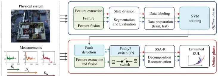
Abstract— This paper presents a condition monitoring approach for point machine prognostics to increase the reliability, availability, and safety in railway transportation industry. The proposed approach is composed of three steps: 1) health indica-tor (HI) construction by data fusion, 2) health state assessment, and 3) failure prognostics. In Step 1, the time-domain features are extracted and evaluated by hybrid and consistency feature evaluation metrics to select the best class of prognostics features. Then, the selected feature class is combined with the adaptive feature fusion algorithm to build a generic point machine HI. In Step 2, health state division is accomplished by time-series segmentation algorithm using the fused HI. Then, fault detection is performed by using a support vector machine classifier. Once the faulty state has been classified (i.e., incipient/starting fault), the single spectral analysis recurrent forecasting is triggered to estimate the component remaining useful life. The proposed methodology is validated on in-field point machine sliding-chair degradation data. The results show that the approach can be effectively used in railway point machine monitoring.

Index Terms— Adaptive feature fusion, feature selection and evaluation, health state division, point machine sliding-chairs, prognostics, segmentation, single spectral analysis, support vector machine (SVM).

I. INTRODUCTION

H

described as an inspection process of the machine degra-dation to detect the health state changes due to anomalies from the condition monitoring (CM) data [1]. Hence, the health state assessment information can be used in the devel-opment of prognostics for complex systems’ monitoring such as high-speed trains [2]–[4] and railway infrastructures, power supply systems [5], overhead contact line [6], [7], and point machines [8].

Railway point machines are one of the complex structures in railway infrastructure, which are used to control the railway turnouts at a given distance [9]. Thus, it is important to monitor the point machine components in order to increase operational Manuscript received April 23, 2018; revised June 25, 2018; accepted August 02, 2018. The Associate Editor coordinating the review process was Roberto Ferrero. (Corresponding author: Kamal Medjaher.)

V. Atamuradov and K. Medjaher are with the Production Engineering Lab-oratory, INP-ENIT, 65000 Tarbes, France (e-mail: vepa.atamuradov@enit.fr; kamal.medjaher@enit.fr).

F. Camci is with AMD Inc., Santa Clara, CA 95054 USA (e-mail: fatih.camci@amd.com).

P. Dersin is with ALSTOM, 93400 Saint-Ouen, France (e-mail:

pierre.dersin@alstomgroup.com).

N. Zerhouni is with the FEMTO-ST Institute, UMR CNRS 6174, UFC/ENSMM, 25000 Besançon, France (e-mail: zerhouni@ens2m.fr).

Color versions of one or more of the figures in this paper are available online at http://ieeexplore.ieee.org.

reliability, availability, and passenger safety [10]. Usually, the general procedure of CM methods includes data preprocessing, i.e., feature extraction, health indicator (HI) construction, health state division, fault detection, and remaining useful life (RUL) estimation steps.

After the extraction of time-based, frequency-based, and time–frequency-based [11] features from the measurements, the feature evaluation and selection are a key step in HI construction. The feature evaluation and selection metrics can be classified as follows.

1) Inherent, which filters the least interesting features using some ranking threshold (e.g., trendability (with time), monotonicity, and seperability [12]).

2) Consistent, which filters the least correlated features from the feature population.

3) Hybrid, which either combines inherent and/or consistent feature evaluation metrics to build a better feature selection scheme [13].

Javed et al. [14] proposed inherent feature selection metrics to evaluate the goodness of features for accurate prognostics of two different real applications. A similar work was also proposed in [15]. This paper is based on the inherent feature evaluation metric integrated with genetic algorithm (GA) to build a good prognostics HI for equipment CM. A linearly weighted hybrid fitness function for prognostics feature selec-tion was proposed in [16]. The proposed method utilizes the GA in the weight optimization step for the combination of features. However, despite the good optimization performance, using heuristic algorithms such as GA in weight optimization step of the hybrid metrics might be computationally expensive, particularly, if there is an increase in the amount of feature size. Moreover, although there are plenty of proposed feature selection metrics in the literature, it is hard to have a generic feature selection technique which is superior to others to build a good component HIs [17]. Thus, the development of more robust and computationally efficient feature evaluation and selection methods is necessary for HI construction to improve the accuracy of CM approaches for prognostics. One of the techniques of building a good HI for component CM is the feature fusion.

The main goal of feature fusion is to construct a generic machine HI to enhance the information content about the system degradation [18]. Since a single feature may contain partial and/or less correlated information about the component degradation [19], it might not include enough information about the component degradation. Therefore, it is beneficial to fuse different features that contain more complementary information about the health state of the degrading machine.

Fig. 1. Proposed CM approach workflow.

A novel fusion approach based on the combination of multiple linear regression models and superstatistics for prog-nostics has been presented in [20]. Lui et al. [21] proposed a composite health index demonstration approach through weighted average fusion using multisensory data for prog-nostics. Similarly, Yan et al. [22] proposed a HI construction approach based on the linear fusion method for asset prog-nostics, which operates under multiple operational conditions. In the same domain, a probabilistic multisensor data fusion approach for machinery CM, based on factoral analysis, was proposed in [23].

Although there are different fusion methods that were proposed for prognostics HI construction, there still remain some challenges in multifeature fusion due to the nonlin-ear degradation of components under different environments. Hence, developing a fusion strategy which can adaptively capture the local degradation changes conditioned to the feature population behavior is necessary. When the com-ponent HI is constructed, the obtained HI can be used in health state division step to discriminate the degradation levels.

The health state division can be defined as an assessment process of a component health status by dividing the HI into discrete degradation levels (e.g., healthy, faulty minor, and faulty critical). A data-driven health assessment methodology was proposed in [24] for failure prognostics of point machines next to health state division. The health state division was carried out by fitting two different degradation functions, and then the divided states were used in RUL estimation. A similar health state division approach using model fit-ting techniques was proposed in [25]. Eker et al. [9] and Eker and Camci [26] proposed a clustering-based health state detection and probabilistic prognostics approach for point machine monitoring. The proposed approach was compared with a hidden Markov model (HMM)-based health state divi-sion. However, HMM-based health state detection is compu-tationally expensive, whereas the clustering-based approaches may not guarantee that the change in health states is due to the machine degradation. Indeed, the clusters, i.e., health states,

found by these tools may refer to variations of the operational conditions rather than the variations due to degradation. Hence, it is important to build a model which is computationally efficient and invariant under the operational conditions. After the health state assessment process, the obtained component state information can be used in fault detection.

Fault detection can be described as a study of the change in component health state magnitudes by measuring the statistics of a fault propagation to characterize them as normal or faulty. In the literature, fault detection and diagnostics have been extensively studied for point machine monitoring by using machine learning [27], [28], signal processing [29], and statis-tical tools [30]–[32]. Lee et al. [33] proposed a fault detection approach for railway point machines based on acoustic data analysis. In this paper, time–frequency-based features were extracted and some of them were selected and used to detect and diagnose faults based on a support vector machine (SVM) classifier. However, traditional supervised fault detection meth-ods need a prior knowledge of the available data labels, which may not be always possible to have such information. Hence, it is preferable to build autonomous fault detection methods, which do not require a prior knowledge of the data in CM.

Based on the state-of-the-art analysis, this paper proposes a CM approach for railway point machine prognostics to fill the aforementioned gaps in the literature, particularly, in HI construction via feature evaluation and selection and fusion, health state assessment, i.e., health state division, and health state detection. For this purpose, the proposed approach, which is illustrated in Fig. 1, is composed of an offline phase and an online phase.

In the offline phase, a new feature evaluation method for prognostics feature selection, composed of hybrid feature selection and consistency parameter ranking, is developed to select the best representative feature class for fusion. In the hybrid feature selection step, an affinity matrix is built from the extracted feature pool and then, the features’ relative importance weights are calculated. Then, inherent metrics such as monotonicity, correlation, and robustness are calculated.

A weighted hybrid fitness function is then constructed by combining the between (i.e., relative importance weights) and within (i.e., inherent metrics) feature evaluation steps to form initial-ranked (i.e., best to worse) prognostics features. Afterward, the ranked features are used in the consistency parameter ranking step. The main goal of the consistency parameter ranking is to select the most consistent feature class among the best features. The selected feature class should have the highest consistency value. A component HI is then built from the consistent feature class by the proposed adaptive feature fusion (AFF) method. The AFF working principle relies on linearly weighted fusion strategy, based on the dynamically changing weights, conditioned to the machine degradation evolution in time.

The obtained HI is then fed into a bottom-up (BUP) time-series segmentation [39] algorithm and a silhouette segment optimization to divide the machine health states. The segmen-tation decomposes the given HI into different health states, whereas the silhouette criterion (SC) [34] evaluates the HI seg-ments to optimize the health states. By using the health state division information, the unlabeled raw measurements can be labeled (e.g., healthy, faulty-medium, and faulty-critical) prior to supervised fault detection. Finally, an SVM classifier [35] is trained by using the labeled raw CM measurements.

In the online phase, once the SVM detects the fault, the fail-ure prognostics algorithm is triggered by using the fused HI. The RUL of the sliding chair is then estimated by using a single spectrum analysis recurrent (SSA-R) forecasting [36] algorithm. The SSA-R is a nonparametric data-driven method based on a combination of statistics, probability theory, and signal processing concepts, which is used in time-series decomposition, identification, and forecasting [37]. In the literature, the SSA-R was used in fault detection [38], [39] and failure prediction [40], [41] of different applications.

The proposed approach is implemented on in-field point machine sliding-chair degradation data, which were col-lected from a real system, to illustrate its effectiveness and applicability.

The main contributions of this paper are as follows. 1) A new HI construction method for point machine

prognostics composed of a hybrid feature selection, a consistency parameter ranking, and an AFF based on a dynamic weight update strategy. Compared to the heuristic methods [16], our feature evaluation method is computationally efficient and effective for machine HI construction.

2) Segmentation-based point machine health state assess-ment (i.e., health state division). The segassess-mentation-based health state division method can detect health state transitions better than clustering-based techniques [9], and it is robust against the nonmonotonicity problem, which is more likely seen in clustering-based health state division methods.

3) An autonomous health state classification regardless of

a prioriknowledge. Compared to traditional supervised methods, our health state classification method relies on an unsupervised data labeling strategy that labels

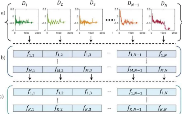
Fig. 2. (a) Raw data (DN is the N th sample). (b) Extracted feature set

( fM,N). (c) Selected feature subset ( fK,N, where K < M).

unlabeled measurements autonomously, regardless of the user intervention.

4) Finally, the application to real data related to railway point machines.

This paper contains four sections after the introduction. Section II explains the proposed approach. The point machine description, the data collection procedure, and the pro-posed approach results are presented in Section III. Finally, Section IV concludes this paper.

II. PROPOSEDAPPROACH

In this section, the offline and online phases of the proposed approach will be explained. The offline phase includes hybrid feature selection and consistency parameter ranking steps, segmentation-based health state division and optimization, and fault detection tool training. The online phase includes fault detection and SSA-R-based failure prognostics for component RUL estimation. The proposed CM approach workflow is shown in Fig. 1.

A. Feature Ranking and Consistency Evaluation

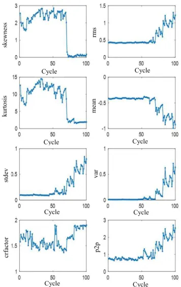
In this paper, time-domain-based features such as skewness, root mean square (rms), kurtosis, mean, standard deviation (stdev), variance (var), crest factor (crfactor), and peak-to-peak (p2p) are extracted from the point machine sliding-chair CM data. The extracted statistical features with different degra-dation behaviors (e.g., increasing or decreasing) in different scales are normalized before the selection step [(1) and (2)]. Equation (1) is used to normalize the features with a decreas-ing trend, whereas (2) is used to normalize the features with an increasing trend. The developed feature evaluation steps are shown in Fig. 2.

Fi =

(Di− min(Di))

(max(Di) − min(Di)); where Di,t =

fi,t max( fi)

(1)

Fi =

(Di− min(Di))

(max(Di) − min(Di)); where Di

,t =

min( fi)

fi,t

(2)

where fi,t is the i th feature data point at time index t (t =

1, . . . , T ), T is the feature length, and Fi is the i th normalized

The hybrid feature selection, that is to rank the best features, is carried out in two steps. In Step 1, the affinity matrix

(4) is built using the Euclidean distance (3) in the following

equation: dist( fp, fq) = ! " " #$N i=1 ( fp,i− fq,i)2 (3)

where N is the length of the given features p and q

Affinity_{M×M =}

%

0 if p_{= q}

dist( fp, fq) if p 6= q

(4)

where dist( fp, fq) is the Euclidean distance between the

fea-tures fpand fq from the feature population with a size of M.

The relative importance weight wi of the i th(∀i = 1 . . . M)

feature is calculated by using the exponential membership function (5). A feature with the minimum interclass distance is assigned with the highest weight (w) value in the feature selection. wi = exp     −1 × M ) i=1 dist( f_i,1) M     . (5)

In Step 2, inherent metrics such as monotonicity (Moni),

correlation (Corri), and robustness (Robi) are calculated

using (7)–(9). Then, a hybrid feature evaluation function is built.

The feature monotonicity metric is used to extract increas-ing or decreasincreas-ing trend information. The feature correlation measures the linearity statistics between the degradation and time. The robustness metric stands for the features’ resistance to the measurement noise. The correlation parameter utilized in this paper is based on Pearson’s correlation coefficient [42].

Moni( fi) = -.._. . . #_{d f}d i> 0 N− 1 − #_{d f}d i< 0 N− 1 . . . . . / (6)

where Moni is the monotonicity value for the i th feature ( fi)

with the length of N . The absolute value of the difference

between the number of positive (#(d/d fi) > 0) and negative

(#(d/d fi) < 0) derivatives gives the monotonicity value.

A feature with the higher monotonicity indicates a better degradation with an increasing/decreasing trend

Corri( fi, Ti) = 0_{cov( f} i, Ti) σfiσTi 1 (7)

where cov is the covariance of the i th feature ( fi) with the

time vector T , and σ is the standard deviation. To calculate the features robustness, first of all, the given feature should be decomposed into the trend and residual components. The

residual component (res fi) of a feature fi is extracted by

subtracting the smoothed feature smoothed_ fi(trend) from the

original (noisy) feature fi, as given in (8). Then, the robustness

is calculated by using (9) res fi = fi− smoothed_ fi (8) Robi( fi) =      N ) n exp2₋.._.res fi fi . . .3 N      (9)

where N is the length of the i th feature ( fi). Then, the features

are ranked by using the hybrid feature ranking function given in (10). The hybrid ranking function is the combination of the inherent metrics weighted by the corresponding relative importance weights.

hybRranking_{i =}

M

$

i=1

[wi× Moni, wi× Corri, wi× Rubi].

(10) Finally, the hybRranking vector is sorted in a descending order starting from the highest relevant feature to the lowest relevant feature. Once the feature ranking step is completed, the ranked features are fed into the consistency evaluation step to select the most consistent feature class for the fusion.

The goal of the feature consistency evaluation can be described as an analysis of the correlation statistics among the given feature set to select the most consistent class of features. In regard to this, the optimal (i.e., the most consistent) class can be obtained by an incremental evaluation method. To do this, the first k number of features is selected. Then,

the consistency parameter Conkis calculated. In each iteration,

the same procedure is repeated by incrementing the value of k by 1, i.e., adding a new feature to the previous class, until the whole feature set is evaluated. Finally, the feature class with the size of K (K < M) can be determined as the optimum consistent class with the maximum consistency parameter.

The Conk parameters are calculated by using the following

equation_:

Conk= exp

0

−std (HIEOL)

mean_{|HIEOL− HI0|}

1

, _{∀k = 2 . . . (M − 1)}

(11)

where HIEOLis a vector including the HI values at the end of

life, and HI0is a vector including the HI values at the initial

time. The selected feature subset is then used to build a unique component HI by using the AFF.

B. Adaptive Feature Fusion

In this section, the proposed AFF method, which is based on the dynamic weight, is described to construct the generic component HI.

Suppose that we have selected the most consistent feature

subset SN×k from the hybrid feature selection step, with k

features (xi, i = 1, . . . , k), where k = max(Con)(11) and

N is the number of observations. Then, the mean distance

vector di (12) between the given feature values xit at time t,

(xi

t, i = 1, . . . , k, t = 1, . . . , N) is calculated as given in (12).

It is obvious that the feature value x_it with the min(d_i) has the

Fig. 3. Simulated features with varying mean distance values.

j _{= 2, . . . k, ) at time t. Therefore, the following weight wi}t

is assigned to x_it, as given in (13). As the feature degradation

behavior changes in time, the weights assigned to each feature value change adaptively, conditioned to the distance parameter between the feature observations.

di(xit) = 1 k_{− 1}× N $ i6= j,t=1 kxit− xtjk2 (12) wt_{i = exp(−1 × d}i). (13)

After the construction of the dynamic weights for the given features at time t, the features are weighted and combined to get the generic HI for prognostics. The final form of the

proposed AFF is given in the following equation_:

Ft = N ) i=1 wi,tfi,t N ) i=1 wi,t = N ) i=1 4 exp -−1 × -1 k−1 × N ) i6= j,t=1 5 5xt i−xtj 5 52 //6 × fi,t N ) i=1 -exp -−1 × -1 k−1 × N ) i6= j,t=1 5 5xt i − x t j 5 52 /// (14)

where Ft is the fused feature at time t (t = 1, . . . , N).

To illustrate the dynamic evolution of the feature values, we have simulated four exponentially degrading features

( f1– f4), as shown in Fig. 3. The vertical solid lines at each

time index indicate the in-between feature values mean dis-tance, which can be referred to error bars. After the fifth cycle,

the variance between f4 and the other features increases and

the length of the error bars changes dynamically. In contrast,

the features f1,2,3 keep the similar pattern of error length,

indicating the correlation in failure propagation. It is most likely that this kind of feature propagations can happen in most applications, assuming that each feature (or sensor) has its distinct physical meaning with the varying failure propagation.

TABLE I

BUP TIMESERIESSEGMENTATIONPSEUDOCODE

Hence, a fusion algorithm should be able to cope with the local changes in failure propagation when constructing the component HI.

After the feature fusion step, the combined generic HI is used in the health state division, which is explained in Section II-C.

C. Segmentation-Based Health State Division and Optimization

In this paper, the BUP time-series segmentation tech-nique [43] is used in health state division. In a BUP segmentation, which is a piecewise linear approximation tech-nique, the two adjacent segments are merged by calculating the cost function. The same procedure is repeated iteratively until a stopping criterion is met. A detailed explanation of the BUP time-series segmentation can be found in [43]. A pseudocode for the BUP algorithm, which is used in this contribution, is shown in Table I.

Since the BUP decomposes the given feature into homoge-nous subsequences, each segment can be treated as a different machine health state with different degradation levels. Thus, the feature segments can be used in machine health assessment for fault detection and prognostics.

Generally, segmentation techniques are supervised and they need a predefined threshold or segment number prior to the segmentation. Therefore, a segment evaluation is needed to optimize the segment numbers and get the best homogeneous segments. In this paper, the optimum segment evaluation is carried out by using a well-known within cluster consistency evaluation technique, which is the SC [34].

The SC, which measures the within-class data consistency, is used to evaluate the optimal number of segments in the health state division.

Let us consider a(i ) as the within-segment mean distance

If Mi ∈ Sk, (k = 1, . . . , K ), then we have a(i ) = 1 nk− 1× $ i6= j d(Mi, Mj) (15)

where K is the total number of segments and nk is the length

of the segment Sk. Next, the mean distance δ(Mi, Sk′) of Mi

to the points of each of the other segments Sk′ is calculated as

δ(Mi, Sk′) = 1

nk′ ×

$

i′_∈Ik′

d(Mi, Mi′) (16)

where Ik′ is the set of observation indices belonging to the

segment Sk′. Then, the smallest mean distance is selected and

denoted as b(i ), as given in (17). The silhouette width for each

point Mi is then calculated by using (18).

b(i ) = min

k′_=kγ (Mi, Sk′) (17)

s_{(i ) =} b(i ) − a(i)

max(b(i ), a(i )) (18)

s(i ) takes the values between −1 and +1 (−1 ≤ s(i) ≤ 1).

A higher value of s(i ) indicates that Mi is well matched to its

segment. If most data points have a higher silhouette value, then the segmentation results are appropriate. Otherwise, if they have a lower value, then the segmentation process may have few or many segments. The final SC for a given segment

number is constructed by using the following equation_:

SC₌ 1 K K $ k=1 µk (19)

where µkis the mean silhouette width for a given segment Sk.

The optimum number of segments in the health state division is then calculated by taking the maximum of the SC in the time-series segmentation.

D. Fault Detection

The SVM classifier is chosen for fault detection due to its good accuracy and capability of performing linear and nonlinear data classification [44], especially on small sample data sets [45].

The initial principle of SVM is to separate given data into distinct two classes by finding an optimum decision hyperplane that maximizes the margin between two imaginary parallel planes (support vectors). In SVM, the kernel function describes the similarity measure of given data points. The ker-nel selection has been accepted as one of the major problems in SVM classification. There are several kernel functions used in SVM-based classifications. In this paper, a polynomial kernel with a degree of 3 is used in the health state detection due to its good classification performance among the others such as quadratic and Gaussian. Interested readers are referred to [46] for more detailed information about SVM with different kernel functions.

E. Failure Prognostics With Single Spectral Analysis Recurrent Forecasting

This section will explain the steps of a basic SSA algorithm for time-series forecasting. The interested readers are referred to [37] for more information about the SSA.

Briefly, the algorithm principle is based on two stages:

decompositionand reconstruction, each with two steps. In the

first stage, the time series Ts _{= {ts}n, n = 1, . . . , N} is

decomposed into several independent components (i.e., trend, periodic oscillatory, and noise). In the second stage, Ts is reconstructed by using the less noisy components.

1) Stage-1: Decomposition: The decomposition is accom-plished in two steps; embedding and singular value decompo-sition (SVD).

Embedding: in this step, the 1-D time series Ts is transformed into a trajectory matrix composed of L-lagged

Xi = (ts1, ts2, . . . , tsi+L−1)T vectors, where K = N − L +1.

The window length L should be assigned with an integer from

the range of 2 _{≤ L ≤ N}7_{2. The trajectory matrix} X , which

is an output of the embedding step, takes the form of Hankel matrix (20): X _{= [X1, . . . XK]} =           ts1 ts2 ts3 . . . tsk ts2 ts3 ts4 . . . tsk+1 ts3 ts4 ... ... ... .. . ... ... ... ... tsL tsL+1 tsL+2 . . . tsN           . (20)

The Hankel matrix has equal elements on the diagonals,

i.e., i _{+ j = constant, i, j are the row and column}

indices.

Singular value decomposition (SVD):This step expands the matrix X by using SVD into a sum of weighted orthogonal

matrices. The expansion of the X(L_{× K ) matrix is obtained}

through the eigen decomposition of the covariance matrix C=

X XT_{. After the eigen decomposition, a set of L eigenvalues}

(λ1 ≥ λ2 ≥ λ3 ≥ . . . ≥ λL ≥ λ0) and the corresponding

U1, U2, . . . UL eigenvectors are obtained. If d = maxi, λi >

0, i.e., the number of nonzero eigenvalues is equal to the rank(X), then the SVD of the trajectory matrix X can be

written as X _{= E1+ E1+ . . . E}d, where Ei = √ λiUiViT and Vi = X T_U i √

λi , (i = 1, . . . , d) is the principal components. The

collection of (√λiUiVi) is defined as the eigentriple of the

trajectory matrix X.

2) Stage-2: Reconstruction: The reconstruction stage of the SSA is accomplished in two steps: grouping and averaging.

Grouping: This step splits the Xi matrices into several X_{I = Xi}

1+ . . . + Xip group matrices, where I = {i1, . . . , ip}.

After getting the SVD of X , the split of the 1, . . . , d indices into the disjoint I1, . . . , Im subsets gives the following form:

X_{= XI}

1 + . . . + XIm (21)

Averaging: In this step, XIj is transformed into a Hankel

matrix to reconstruct the original time series through the diagonal averaging or by the “Hankelization” process H().

Let us assume that si j is an element of the generic matrix S,

then the nth term of the reconstructed series is obtained by

averaging the si j over all i, j , such that i + j = n + 2.

H_{(S) can be referred as the reconstructed time series from}

S matrix with the size of N . By applying the “Hankelization”

to all X _{= X}I1 + . . . + XIm, we obtain the expanded X =

H(XI1) + . . . + H (XIm). This procedure is equivalent to the

decomposition of the original series T s _{= {ts}n, n = 1 . . . N}

into a sum of m series: tst = )mk=1T s˜

k

t(t = 1, . . . N),

where ˜T s(k)_{N = { ˜}ts(k)₁ ,ts˜(k)₂ , . . . ,ts˜(k)_N corresponds to the matrix

H (XIk).

The SSA-R algorithm, which is used in forecasting, will be presented hereafter.

a) SSA-R forecasting: The main principle of the SSA-R forecasting tool is based on the linear recurrent relation (LRR). To perform the SSA-R forecasting, the given time series

T s _{= {ts}n, n = 1 . . . N} satisfies an LRR of order d if

there exist the coefficients a1, . . . ad, such that: T si+d =

)d

k=1akT si−d+k, N − d ≥ i ≥ a, ak 6= 0 and d < N.

The coefficients (weights), which are used in the SSA-R forecasting, are obtained from the eigenvectors in the SVD step [47]. The future values of the reconstructed time series can be predicted by choosing the first r eigentriples.

Let E be the chosen numbers of eigentriples, Ui ∈ RL and

i _{∈ E are the eigenvectors, ¯}Ui ∈ RL−1is the L−1 component

vector of the Ui, ρi be the last component of Pi,v2 =

)

i∈Eρi2, and 8T sN = {9ts1, . . ., ts8nbe the reconstructed series

by E. We define L = span(Ui, i ∈ E) as the linear space

spanned by Ui in an orthonormal base (i.e., which is not a

vertical space). Suppose that /_{∈ e}LL, eL = (0, 0, . . . , 1)T and

v2_{< 1. Then, it can be proven that the last component y}

L of

any vector F _{= ( f1, f2, . . . , f}L)T ∈ L is a linear combination

of the first components, i.e., f1, f2, . . . , fL−1(yL= a1fL−1+ . . . + aL−1f1), where R = (aL−1, . . . , a1)T is defined as:

R₌ 1

1− v2

$

i∈E

ρiU¯i. (22)

The h-step ahead prediction of the time series ZN+h =

{z1, z2, . . . , zN+h} can be obtained by:

zi=        ˜ tsi, i = 1, . . . , N L−1 $ j=1 ajzi− j, i = N + 1, . . . , N + h. (23)

The zN+1, . . . , zN+h values are the h-step ahead predictions of the time series Z .

Note that the selection of the parameters L (window length) and r (number of components) is very important in the SSA. A detailed information about the selection of the parameters can be found in [47].

b) RUL prediction: Before the RUL prediction, the HI, taken as a time series, is divided into two sets: training and testing. The training set is used to tune the SSA-R algorithm, while the testing set is used to estimate the RUL. In this paper, the training sample includes the healthy state time series, whereas the testing sample includes the faulty and the critical state time series.

The estimated RUL (eRULp) of the sliding-chair plate

degradation, at each prediction point ( p_{= N, N +1, . . . N +i;}

p_{≤ CEOL), is calculated as:}

eRULp= CEOL−

M

$

m

(Fm ≤ EOLT) (24)

where N is the initial prediction time, CEOLis the component

failure time, Fm is the predicted series with length m, EOLT

is the failure threshold, and i is the prediction step. The RUL estimation is based on the one-step-ahead prediction.

III. APPLICATION ANDRESULTS

A. System Description and Data Collection

Since point machines are one of the complex systems of the railway infrastructure, they have many failure modes such as the dry sliding chair, locking system, motor state, clutch slipping, and electric peripheral wear [48].

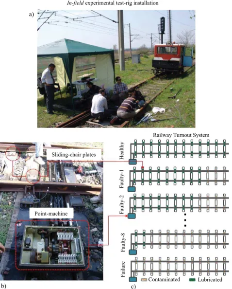
This paper investigates the dry sliding-chair failure mode of the point machine, which has been generated by an accel-erated aging procedure. Briefly, this aging can be defined as a manual contamination process (i.e., soiling or scratch-ing out the grease) of the slidscratch-ing-chair plates to obtain the slowly progressive failure modes in a short period of time. Fig. 4 shows the in-field experimental test-rig setup [Fig. 4(a)], the point machine [Fig. 4(b)], and the accelerated sliding-chair degradation modeling procedure [Fig. 4(c)] on the turnout with 12 wooden traverses (Tr.).

Sliding-chair plates are the metal assets of the turnout system that assist the point machine drive rods in moving the rail blades easily. The sliding-chair degradation data were collected from the real Turkish State Railways point machine in Tekirda˘g, Turkey. This turnout system has 12 sliding-chair plates in total. At first, all the 12 plates were individually lubricated and the point machine was run 10 times in each movement to get the first healthy (fault-free) CM sensory data. Afterward, the contamination (sprinkling dust or sand)

process took place by soiling three farthest (10th, 11th, and

12th) sliding-chair plates from the point machine to get an

initial faulty state. The second faulty state was created by soiling the ninth sliding-chair plate after the first contamination process. The accelerated failure process was repeated until a final and complete sliding-chair failure state was created. After each step of the contamination process, the point machine was run 10 times from normal-to-reverse (forth) and reverse-to-normal (back) positions to collect the sensory data. The contamination on the sliding-chair plates results in a variation of the performance measurement signals (e.g., force, current, voltage, and so on) due to the increasing friction force against the turnout driving rod force applied to move the blades from normal-to-reverse (forth) or reverse-to-normal (back) positions. The total number of degradation data collected in each state is 20 (10 in back and 10 in forth movements). Note that no trains went through the turnout system during the data acquisition operation. The turnout system was temporarily reserved as an experimental point machine for the sliding-chair failure modeling and data collection purposes only.

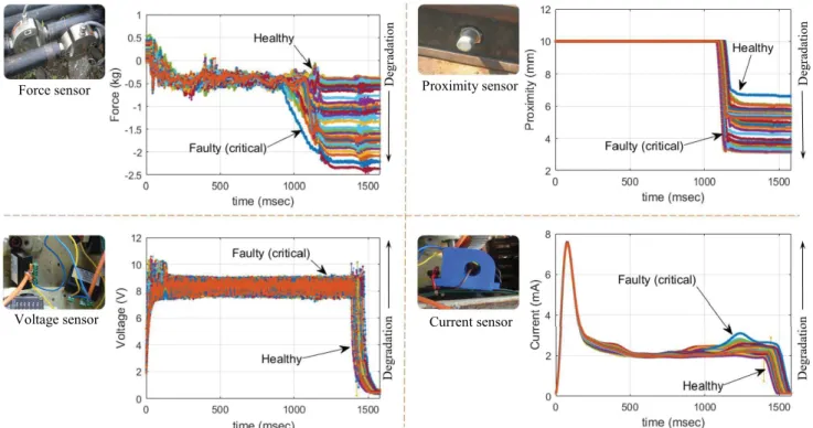
Fig. 4. (a) Experimental test-rig installation, (b) Point Machine and (c) Degradation modeling. Different sensors (see Fig. 5) were installed on the

electro-mechanical point machine components (e.g., drive rods, cables, rails, and so on) to monitor and collect degradation data. Fig. 5 shows the collected force, DC current, voltage, and proximity sensor data from the point machine. The CM data collected by the force and current sensors are the most commonly used sensors in the literature for point machine diagnostics and prognostics [48]. In this paper, the force degradation data are used to validate the proposed approach.

B. Results and Discussion

1) Feature Selection and Fusion:Fig. 6 shows the extracted time-domain-based statistical features from the raw force measurements, and Fig. 7 illustrates the normalized features by using (1) and (2).

The hybrid feature selection was carried out in two steps. In Step 1 (Table II), the affinity matrix and the relative features importance weights were calculated using (4) and (5). In Step 2 (Table III), inherent metrics such as monotonicity, correlation, and robustness were calculated using (6), (7), and (9). Before calculating the monotonicity metric, the features

TABLE II

INTERCLASSFEATUREANALYSIS AND THECALCULATED

RELATIVEIMPORTANCEWEIGHTS(w) (STEP1)

are smoothed by utilizing the moving average (MA) technique. Step 1 results are shown in Table II, and Table III presents the ranked features (F1{skewness}, F2{kurtosis}, F3{rms}, F4{mean}, F5{stdev}, F6{var}, F7{crfactor}, and F8{p2p}) after the hybrid ranking (hybRanking). Then, the ranked fea-tures were fed into the consistency evaluation step to select the best-correlated feature class.

Fig. 5. Sensors and collected measurements.

TABLE III

INTRACLASSFEATUREANALYSIS AND THE CALCULATEDHYBRIDFIT

-NESSFUNCTION(hybRanking) RESULTS(STEP2)

In the consistency evaluation step, the first k _{= 2 number}

of features, i.e., F3 and F5, were selected and the parameter

Conk=2 was calculated. In each iteration, the same procedure

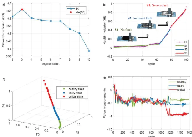
was repeated by incrementing the value of k by one until the whole feature set was evaluated. Then, the feature subset with the maximum consistency metric (11) was selected as the best-correlated feature subset. The calculated consistency parameters are given in Fig. 8(a), whereas Fig. 8(b) shows the selected feature class, which has the highest Con.

Afterward, the selected feature class was used to build an HI by using the AFF algorithm. Fig. 8(e) shows the fused HI result, whereas Fig. 8(c) and (d) shows the distance values and the dynamically adapted weights for the given HI observations. In summary, the AFF algorithm can detect the features’ local variations adaptively while constructing the global HI of the degrading component.

2) Health State Assessment: Health State Division and Labeling: The constructed HI is then fed into the BUP, and silhouette segment evaluation to divide and optimize the sliding-chair health states. First of all, the fused HI was

denoised by utilizing the MA technique to reduce the noise impact on the segmentation and optimization steps. The BUP segmentation algorithm was run several times using different segment numbers, starting from 2 up to 10. After each seg-mentation process, the SC was calculated. The maximum SC was obtained in the second segmentation process, by initial-izing the BUP with the number 3. Fig. 9 shows the health state division and optimization results. The SC results are shown in Fig. 9(a), and the segmentation results with fault severity information (S1—no fault, S2—incipient fault, and S3—severe fault) are shown in Fig. 9(b). The sliding-chair degradation state transitions in the representation space [35] are shown in Fig. 9(c), whereas the raw data samples from each health state are shown in Fig. 9(d).

After the segment evaluation process, the raw force time series were labeled. The assigned data labels to the force measurements are shown in Table IV. The first 72 force mea-surements were labeled as “healthy”, meamea-surements between 73 and 78 as “faulty” and measurements between 79 and 100 as “critical” health states for the sliding-chair degrada-tion. Then, the fault detection algorithm was trained. Note that the proposed autonomous health state assessment method does not need any prior knowledge of the data labels in fault detection.

3) Fault Detection and Prognostics: By using the labeled force measurements, the SVM was trained in the offline phase and was tested in the online phase for fault detection. The main focus of this step is to perform multiclass classification using the SVM to detect the faulty force time series and identify the triggering point for prognostics.

Fig. 6. Extracted time-domain features from force time series.

Fig. 7. Normalized time-domain features.

The fault detection was performed using two different scenarios. Scenario-1 includes the healthy, the faulty, and the critical force data classes. Scenario-2 includes only the healthy and the faulty force data classes. By using these scenarios,

TABLE IV

DEGRADATIONSTATES AND THECORRESPONDINGLABELS

TABLE V

MULTISTATECLASSIFICATIONRESULTS FORFAULTDETECTION

the fault detection based on the learned SVM was performed and its performance in two cases was compared. To do this, a 10-fold cross-validation was used in the SVM model training step. The raw force data set was split into different training (50% and 70%) and testing (50% and 30%) samples. The data samples used in model training (MTr) and testing (MTs) were selected randomly in each trial. The training (MTr_acc) and testing (MTs_acc) accuracy values are the mean values of 10 iterations for the corresponding training and testing steps.

The sliding-chair fault detection results are shown

in Table V. In Scenario-1, due to less variance between the health state transitions such as healthy, faulty, and critical classes, the classification results are not as accurate as in Scenario-2. Indeed, in Scenario-2, the healthy and faulty classes were classified very accurately by the SVM in both training samples. The Scenario-1 results can be evaluated in a component fault severity assessment and prognostics, whereas Scenario-2 results can be only used to detect an incipient fault to trigger the prognostics algorithm for RUL prediction. In summary, multistate classification based on the SVM for fault detection could classify the states easily by using the raw force data. Once the faulty state is detected by SVM, the SSA-R forecasting is triggered to predict the RUL of the point machine sliding-chair plates.

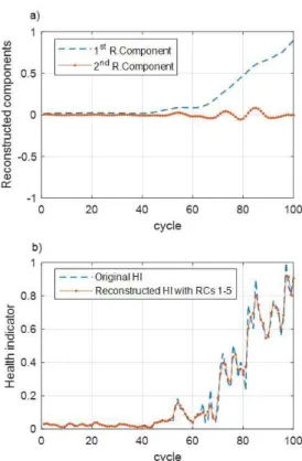
First of all, before the forecasting step, the L and r parameters in the decomposition and reconstruction stages of the SSA-R algorithm are initialized. The window length L was initialized to 10, and r was initialized to 5. Fig. 10(a) shows the first two reconstructed components of the HI, and Fig. 10(b) shows the completely reconstructed HI by using the initialized parameters. Note that using all the components in the HI reconstruction decreases the information contribution while increasing the noise impact. Therefore, in this paper, only the first five-components were used in the reconstruction and prediction.

Initially, the first 72-time series, i.e., series in the healthy state, of the fused HI were considered as the training data

Fig. 8. (a) Consistency (Con). (b) Selected feature class. (c) Distance. (d) Weights (w). (e) Fused HI.

Fig. 9. (a) Silhouette (SC). (b) Optimum segments. (c) Space representation of health state transitions. (d) Force measurements from each state.

set, and the rest as the testing (28-time series) data sets, i.e., series in the faulty and critical states, for RUL estimation. Since the RUL estimation is based on one-step (cycle) ahead

prediction, the length of the training sample is increased in each prediction, and the SSA-R was trained again as new data points are added. Fig. 11 shows the RUL estimation

Fig. 10. (a) First two reconstructed components.(b) Reconstructed HI by

using the r= 5.

Fig. 11. RUL estimation results at each prediction ( p= 73, . . . 100) time

for the sliding-chair degradation.

results at each prediction time ( p_{= 73, 74, . . . , 100) for the}

sliding-chair degradation. As shown in Fig. 11(b), the RUL

estimation errors (r RUL_{− eRUL) in the health state-2 (i.e.,}

the degradation stage of the sliding chairs) is higher than the estimated RULs in the health state-3. This is due to less information that was provided to the SSA-R in the training step. But, again data are available to train the SSA-R, the RUL estimation error decreases [dashed line in Fig. 11(a) and (b)] and the estimated RUL (eRUL) converges to the real RUL (r RUL). Despite the poor RUL estimation results in the health state-2 by the SSA-R, the RUL estimation results are improved in the health state-3.

IV. CONCLUSION

In this paper, a CM approach for fault detection and prognostics of sliding-chair failure was proposed.

In the offline phase, a goodness of prognostics features was evaluated by the proposed hybrid and consistency evaluation metrics to select the best feature class for fusion. Then, the selected feature class was fused by the proposed AFF fusion algorithm to build a generic component HI. After fusion, the HI was fed into the health state assessment for health state division and data labeling steps. The health states were segmented by using the BUP time-series segmentation algorithm, whereas the segments were optimized by using the SC. After the data labeling process, the labeled force time series were used in the training and testing steps of the SVM for fault detection.

In the online phase, once the faulty state is detected by the SVM classifier, the SSA-R algorithm was triggered to predict the point machine RUL by using the fused HI. The results show that the proposed approach for railway point machine CM can be effectively used in the evaluation of prognostics features and can be applied for online fault detection and prognostics.

As a future work, it is planned to use different prognostics tools in the RUL estimation problem. Furthermore, the results will be integrated with the development of a post-prognostics method to support better decision making in component main-tenance planning.

REFERENCES

[1] M. Cerrada et al., “A review on data-driven fault severity assessment in rolling bearings,” Mech. Syst. Signal Process., vol. 99, pp. 169–196, Jan. 2018.

[2] L. Liu, F. Zhou, and Y. He, “Automated visual inspection system for bogie block key under complex freight train environment,” IEEE Trans.

Instrum. Meas., vol. 65, no. 1, pp. 2–14, Jan. 2016.

[3] H. Henao, S. H. Kia, and G.-A. Capolino, “Torsional-vibration assess-ment and gear-fault diagnosis in railway traction system,” IEEE Trans.

Ind. Electron., vol. 58, no. 5, pp. 1707–1717, May 2011.

[4] V. Atamuradov, K. Medjaher, P. Dersin, B. Lamoureux, and N. Zerhouni, “Prognostics and health management for maintenance practitioners— Review, implementation and tools evaluation,” Int. J. Prognostics Health

Manag., vol. 8, no. 3, pp. 1–31, 2017.

[5] S. Saponara, L. Fanucci, F. Bernardo, and A. Falciani, “Predictive diagnosis of high-power transformer faults by networking vibration mea-suring nodes with integrated signal processing,” IEEE Trans. Instrum.

Meas., vol. 65, no. 8, pp. 1749–1760, Aug. 2016.

[6] J. Chen, Z. Liu, H. Wang, A. Nunez, and Z. Han, “Automatic defect detection of fasteners on the catenary support device using deep con-volutional neural network,” IEEE Trans. Instrum. Meas., vol. 67, no. 2, pp. 257–269, 2017.

[7] M. Brahimi, K. Medjaher, M. Leouatni, and N. Zerhouni, “Prognostics and health management for an overhead contact line system—A review,”

[8] M. Vileiniskis, R. Remenyte-Prescott, and D. Rama, “A fault detection method for railway point systems,” Proc. Inst. Mech. Eng. F, J. Rail

Rapid Transit, vol. 230, no. 3, pp. 852–865, 2015.

[9] O. F. Eker, F. Camci, A. Guclu, H. Yilboga, M. Sevkli, and S. Baskan, “A simple state-based prognostic model for railway turnout systems,”

IEEE Trans. Ind. Electron., vol. 58, no. 5, pp. 1718–1726, May 2011. [10] V. Atamuradov, F. Camci, S. Baskan, and M. Sevkli, “Failure diagnostics

for railway point machines using expert systems,” in Proc. IEEE Int.

Symp. Diagnostics Electr. Mach. Power Electron. Drives (SDEMPED), Aug. 2009, pp. 1–5.

[11] L. Ciabattoni, F. Ferracuti, A. Freddi, and A. Monteriu, “Statistical spectral analysis for fault diagnosis of rotating machines,” IEEE Trans.

Ind. Electron., vol. 65, no. 5, pp. 4301–4310, May 2017.

[12] F. Camci, K. Medjaher, N. Zerhouni, and P. Nectoux, “Feature evaluation for effective bearing prognostics,” Qual. Reliab. Eng. Int., vol. 29, no. 4, pp. 477–486, 2013.

[13] Y. Lei, N. Li, L. Guo, N. Li, T. Yan, and J. Lin, “Machinery health prog-nostics: A systematic review from data acquisition to RUL prediction,”

Mech. Syst. Signal Process., vol. 104, pp. 799–834, May 2018. [14] K. Javed, R. Gouriveau, N. Zerhouni, and P. Nectoux, “Enabling

health monitoring approach based on vibration data for accurate prog-nostics,” IEEE Trans. Ind. Electron., vol. 62, no. 1, pp. 647–656, Jan. 2015.

[15] L. Liao, “Discovering prognostic features using genetic programming in remaining useful life prediction,” IEEE Trans. Ind. Electron., vol. 61, no. 5, pp. 2464–2472, May 2014.

[16] J. Coble and J. W. Hines, “Identifying optimal prognostic parameters from data: A genetic algorithms approach,” in Proc. Annu. Conf.

Prognostics Heal. Manag. Soc., 2009, pp. 1–11.

[17] C. Freeman, D. Kuli´c, and O. Basir, “An evaluation of classifier-specific filter measure performance for feature selection,” Pattern Recognit., vol. 48, no. 5, pp. 1812–1826, 2015.

[18] Z. Chen and W. Li, “Multisensor feature fusion for bearing fault diagnosis using sparse autoencoder and deep belief network,” IEEE

Trans. Instrum. Meas., vol. 66, no. 7, pp. 1693–1702, Jul. 2017. [19] V. Atamuradov and F. Camci, “Segmentation based feature evaluation

and fusion for prognostics feature selection based on segment eval-uation,” Int. J. Prognostics Heal. Manag., vol. 8, no. 2, pp. 1–14, Dec. 2017.

[20] J. Lui, M. Zhang, H. Zuo, and J. Xie, “Remaining useful life prognostics for aeroengine based on superstatistics and information fusion,” Chin.

J. Aeronoutics, vol. 27, no. 5, pp. 1086–1096, 2014.

[21] K. Lui, N. Z. Gabraeel, and J. Shi, “A data-level fusion model for developing composite health indices for degradation modeling and prognostic analysis,” IEEE Trans. Autom. Sci. Eng., vol. 10, no. 3, pp. 652–664, Jul. 2013.

[22] H. Yan, K. Liu, X. Zhang, and J. Shi, “Multiple sensor data fusion for degradation modeling and prognostics under multiple operational condi-tions,” IEEE Trans. Reliab., vol. 65, no. 3, pp. 1416–1426, Aug. 2016. [23] J. Wang, J. Xie, R. Zhao, K. Mao, and L. Zhang, “A new probabilistic kernel factor analysis for multisensory data fusion: Application to tool condition monitoring,” IEEE Trans. Instrum. Meas., vol. 65, no. 11, pp. 2527–2537, Nov. 2016.

[24] C. Letot et al., “A data driven degradation-based model for the mainte-nance of turnouts: A case study,” IFAC-PapersOnLine, vol. 28, no. 21, pp. 958–963, 2015.

[25] M. Ma, C. Sun, and X. Chen, “Discriminative deep belief networks with ant colony optimization for health status assessment of machine,” IEEE

Trans. Instrum. Meas., vol. 66, no. 12, pp. 3115–3125, Dec. 2017. [26] O. F. Eker and F. Camci, “State-based prognostics with state duration

information,” Qual. Rel. Eng. Int., vol. 29, no. 4, pp. 465–476, 2013. [27] O. F. Eker, F. Camci, and U. Kumar, “SVM based diagnostic

on railway turnouts,” Int. J. Performability Eng., vol. 8, no. 3, pp. 289–298, May 2012.

[28] F. P. García-Mírquez, C. Roberts, and A. M. Tobias, “Railway point mechanisms: Condition monitoring and fault detection,” Proc. Inst.

Mech. Eng. F, J. Rail Rapid Transit, vol. 224, no. 1, pp. 35–44, 2010. [29] T. Asada, C. Roberts, and T. Koseki, “An algorithm for improved

performance of railway condition monitoring equipment: Alternating-current point machine case study,” Transp. Res. C, Emerg. Technol., vol. 30, pp. 81–92, 2013.

[30] N. Bolbolamiri, M. S. Sanai, and A. Mirabadi, “Time-domain stator current condition monitoring: Analyzing point failures detection by Kolmogorov–Smirnov (K-S) test,” Int. J. Electr. Comput. Energ.

Elec-tron. Commun. Eng., vol. 6, no. 6, pp. 587–592, 2012.

[31] S. Yoon, J. Sa, Y. Chung, D. Park, and H. Kim, “Fault diagnosis of railway point machines using dynamic time warping,” Electron. Lett., vol. 52, no. 10, pp. 818–819, 2016.

[32] V. Atamuradov, K. Medjaher, B. Lamoureux, P. Dersin, and N. Zerhouni, “Fault detection by segment evaluation based on inferential statistics for asset monitoring,” in Proc. Annu. Conf. Prognostics Health Manage.

Soc., 2017, pp. 1–10.

[33] J. Lee, H. Choi, D. Park, Y. Chung, H. Y. Kim, and S. Yoon, “Fault detection and diagnosis of railway point machines by sound analysis,”

Sensors, vol. 16, no. 4, p. 549, 2016.

[34] P. J. Rousseeuw, “Silhouettes: A graphical aid to the interpretation and validation of cluster analysis,” J. Comput. Appl. Math., vol. 20, pp. 53–65, Nov. 1987.

[35] A. Soualhi, K. Medjaher, and N. Zerhouni, “Bearing health monitor-ing based on Hilbert–Huang transform, support vector machine, and regression,” IEEE Trans. Instrum. Meas., vol. 64, no. 1, pp. 52–62, Jan. 2015.

[36] R. Vautard and M. Ghil, “Singular spectrum analysis in nonlinear dynamics, with applications to paleoclimatic time series,” Phys. D,

Nonlinear Phenom., vol. 35, no. 3, pp. 395–424, 1989.

[37] J. Harmouche, D. Fourer, F. Auger, P. Borgnat, and P. Flandrin, “The sliding singular spectrum analysis: A data-driven nonstationary signal decomposition tool,” IEEE Trans. Signal Process., vol. 66, no. 1, pp. 251–263, Jan. 2018.

[38] S. Krishnannair and C. Aldrich, “Fault detection in the tennessee eastman benchmark process with nonlinear singular spectrum analysis,”

IFAC-PapersOnLine, vol. 50, no. 1, pp. 8005–8010, 2017.

[39] B. Kilundu, X. Chiementin, and P. Dehombreux, “Singular spectrum analysis for bearing defect detection,” J. Vib. Acoust., vol. 133, no. 5, p. 051007, 2011.

[40] N. Safari, C. Y. Chung, and G. C. D. Price, “novel multi-step short-term wind power prediction framework based on chaotic time series analysis and singular spectrum analysis,” IEEE Trans. Power Syst., vol. 33, no. 1, pp. 590–601, Jan. 2017.

[41] C. M. S. Rocco, “Singular spectrum analysis and forecasting of failure time series,” Rel. Eng. Syst. Saf., vol. 114, no. 1, pp. 126–136, 2013. [42] G. Chandrashekar and F. Sahin, “A survey on feature selection methods,”

Comput. Elect. Eng., vol. 40, no. 1, pp. 16–28, Jan. 2014.

[43] E. Keogh, S. Chu, D. Hart, and M. Pazzani, “Segmenting time series: A survey and novel approach,” in Proc. Data Min. Time Ser. Databases, 2003, pp. 1–21.

[44] T. R. Baitharu, S. K. Pani, and S. Dhal, “Comparison of Kernel selection for support vector machines using diabetes dataset,” J. Comput. Sci.

Appl., vol. 3, no. 6, pp. 181–184, 2015.

[45] L. Ren, W. Lv, S. Jiang, and Y. Xiao, “Fault diagnosis using a joint model based on sparse representation and SVM,” IEEE Trans. Instrum.

Meas., vol. 65, no. 10, pp. 2313–2320, Oct. 2016.

[46] Z. Yin and J. Hou, “Recent advances on SVM based fault diagnosis and process monitoring in complicated industrial processes,”

Neurocomput-ing, vol. 174, pp. 643–650, Jan. 2016.

[47] N. Golyandina, V. Nekrutkin, and A. A. Zhigljavsky, Analysis of Time

Series Structure: SSA and Related Techniques. Boca Rotan, FL, USA: CRC Press, 2001. [Online]. Available: www.crcpress.com

[48] F. P. García-Márquez and F. Schmid, “A digital filter-based approach to the remote condition monitoring of railway turnouts,” Rel. Eng. Syst.

Safety, vol. 92, no. 6, pp. 830–840, 2007.

Vepa Atamuradov (M’18) received the B.S. degree

in computer technologies from International Black Sea University, Tbilisi, Georgia, in 2007, the M.S. degree in computer engineering from Fatih Univer-sity, Istanbul, Turkey, in 2009, and the Ph.D. degree in electrical-computer engineering from Selçuk Uni-versity, Konya, Turkey, in 2016.

He was involved in research projects Development of Failure Prognostics and Maintenance Planning System for Point Mechanisms in Railway from 2008 to 2009 and Development of Design-Based State-of-Health and Remaining Useful Life Estimation Techniques for Battery Management Systems and Its Application to Rechargeable Batteries from 2014 to 2016, granted by the Scientific and Technological Research Council of Turkey. Since 2016, he has been a Post-Doctoral Research Fellow on prognostics and health management of high-speed train bogies with the Tarbes National School of Engineering (ENIT), Tarbes, France. His current research interests include failure diagnostics and prognostics of complex industrial systems using machine learning and statistical methods.

Kamal Medjaher (M’18) received the Engineering

degree in electronics from Mouloud Mammeri University, Tizi Ouzou, Algeria, the M.S. degree in control and industrial computing from the Ecole

Centrale de Lille, Villeneuve-d’Ascq, France,

in 2002, and the Ph.D. degree in control and industrial computing from the University of Lille 1, Villeneuve-d’Ascq, in 2005.

He was an Associate Professor with the National

Institute of Mechanics and Microtechnologies,

Besançon, France, and the FEMTO-ST Institute, Besançon, from 2006 to 2016. He is currently a Full Professor with the Tarbes National School of Engineering (ENIT), Tarbes, France. He also conducts his research activities within the Production Engineering Laboratory. His current research interests include prognostics and health management of industrial systems and predictive maintenance.

Fatih Camci (M’18) was involved in research

projects related to decision support systems on Prognostics and Health Management (PHM) and energy in USA, Turkey, U.K., and France. He is currently the Manager of IT architecture with AMD, Santa Clara, CA, USA. His current research inter-ests include decision support systems in industrial engineering field focusing on PHM.

Pierre Dersin (M’18) received the B.S. degrees in

engineering and mathematics from Brussels Univer-sity, Belgium, and the M.S. degree in operations research, and the Ph.D. degree in electrical engineer-ing from MIT, Cambridge, MA, USA, in 1980.

He was with MIT LIDS, where he studied the reliability of electric power grids, as part of the Large Scale System Effectiveness Analysis Pro-gram funded by the U.S. Department of Energy. He was with Engineering Firm Fabricom, where he focused on fault diagnostic systems for factory automation. Since 1990, he has been with ALSTOM Transport, where he occupied several positions in reliability-availability-maintainability-safety, Maintenance and Research and Development. Since 2014, he has been the Co-Director of the joint ALSTOM-INRIA Research Laboratory for digital technologies applied to mobility and energy. He is currently the RAM Director and the Prognostics and Health Management (PHM) Director of ALSTOM Digital Mobility, and also the Leader of ALSTOM’s Reliability & Availability Core Competence Network. His current research interests include the links between reliability engineering and PHM and the application of data science, machine learning, and statistics to both fields, as well as systems optimization and simulation, including systems of systems.

Dr. Dersin is the IEEE Reliability Society Administrative Committee Mem-ber and the IEEE Future Directions Committee MemMem-ber. Since 2017, he has been the IEEE Reliability Society Vice President for Technical Activities. He was a Keynote speaker at the Second European PHM Conference, Nantes, in 2014.

Noureddine Zerhouni (M’18) received the

Engi-neering degree from the National Engineers and Technicians Institute of Algiers, Algiers, Algeria, in 1985, and the Ph.D. degree in automatic control from the Grenoble National Polytechnic Institute, Grenoble, France, in 1991.

In 1991, he joined the National Engineering Insti-tute of Belfort, Belfort, France, as an Associate Professor. Since 1999, he has been a Full Profes-sor with the National Institute in Mechanics and Micro technologies, Besançon, France. He has been involved in various European and national projects on intelligent maintenance systems. He is currently a member of the Department of Automatic Control and Micro-Mechatronic Systems, FEMTO-ST Institute, Besançon. His current research interests include intelligent maintenance, and prognostics and health management.