To link to this article : DOI :
10.1007/s41095-016-0075-z
URL :
https://doi.org/10.1007/s41095-016-0075-z
To cite this version :
Bähr, Martin and Breuss, Michael and Quéau, Yvain and
Boroujerdi, Ali Sharifi and Durou, Jean-Denis Fast and Accurate Surface
Normal Integration on Non-Rectangular Domains. (2017) Computational
Visual Media, vol. 3 (n° 2). pp. 107-129. ISSN 2096-0433
O
pen
A
rchive
T
OULOUSE
A
rchive
O
uverte (
OATAO
)
OATAO is an open access repository that collects the work of Toulouse researchers and
makes it freely available over the web where possible.
This is an author-deposited version published in :
http://oatao.univ-toulouse.fr/
Eprints ID : 18856
Any correspondence concerning this service should be sent to the repository
administrator:
[email protected]
Fast
and
accurate
surface
normal
integration
on
non-rectangular domains
Martin B¨ahr1, Michael Breuß1 ( ), Yvain Qu´eau2, Ali Sharifi Boroujerdi1, and Jean-Denis
Durou3
Abstract The integration of surface normals for the purpose of computing the shape of a surface in 3D space is a classic problem in computer vision. However, even nowadays it is still a challenging task to devise a method that is flexible enough to work on non-trivial computational domains with high accuracy, robustness,
and computational efficiency. By uniting a classic
approach for surface normal integration with modern computational techniques, we construct a solver that fulfils these requirements. Building upon the Poisson integration model, we use an iterative Krylov subspace solver as a core step in tackling the task. While such a method can be very efficient, it may only show its full potential when combined with suitable numerical preconditioning and problem-specific initialisation. We perform a thorough numerical study in order to identify an appropriate preconditioner for this purpose. To provide suitable initialisation, we compute this initial state using a recently developed fast marching integrator. Detailed numerical experiments illustrate the benefits of this novel combination. In addition, we show on real-world photometric stereo datasets that the developed numerical framework is flexible enough to tackle modern computer vision applications.
Keywords surface normal integration; Poisson integration; conjugate gradient method;
1 Brandenburg Technical University, Institute for Mathematics, Chair for Applied Mathematics, Platz der Deutschen Einheit 1, 03046 Cottbus, Germany. E-mail: M. B¨ahr, [email protected]; M. Breuß, [email protected] ( ); A. S. Boroujerdi, ali. [email protected].
2 Technical University Munich, 85748 Garching, Germany. E-mail: [email protected].
3 Universit´e de Toulouse, IRIT, UMR CNRS 5505, Toulouse, France. E-mail: [email protected].
preconditioning; fast marching method; Krylov subspace methods; photometric stereo; 3D reconstruction
1
Introduction
The integration of surface normals is a fundamental task in computer vision. Classic examples of processes where this technique is often applied are image editing [1], shape from shading as analysed by Horn [2], and photometric stereo (PS) for which we refer to the pioneering work of Woodham [3]. Modern applications of PS include facial recognition [4], industrial product quality control [5], object preservation in digital heritage [6], and new utilities with potential use in the video (game) industry and robotics [7], among many others.
In this paper we consider surface normal integration in the context of the PS problem, which serves as a role model for potential applications. The task of PS is to compute the 3D surface of an object from multiple images of the same scene under different illumination conditions. The standard PS method for reconstructing an unknown surface has two stages. In a first step, the surface is represented as a field of surface normals, or equivalently, a corresponding gradient field. In a subsequent step this is integrated to obtain the depth of the surface. To handle the integration step, many different approaches and methods have been developed during recent decades. However, despite all these developments there is still the need for approaches that combine a high accuracy reconstruction with
robustnessagainst noise and outliers, and reasonable computational efficiency for working with
high-resolution cameras and corresponding imagery.
Computational issues. Let us briefly elaborate
on the demands on an ideal integrator. As discussed, e.g., in Ref. [8], a practical issue is robustness with respect to noise and outliers. Since computer vision processes such as PS rely on simplified assumptions that often do not hold for realistic illumination and surface reflectance, artefacts may often arise when estimating surface normals from real-world input images. Therefore, the determined depth gradient field is not noise-free and may also contain outliers. These may strongly influence the integration process. Secondly, objects to be reconstructed in 3D are typically in the centre of a photographed scene. Therefore, they only form part of each input image. The sharp gradient usually representing the transition from foreground to background is a difficult feature for most surface normal integrators and generally influences the estimated shape of the object of interest. Because of this it is desirable to consider only image segments that represent the object of interest and not the background. Although similar difficulties (sharp gradients) also arise for discontinuous surfaces that may appear at self-occlusions of an object [9], we do not tackle this issue in the present article. Instead, we neglect self-occlusion and focus on reconstructing a smooth surface on the (possibly non-rectangular) subset of the image domain representing the object of interest. Related to this point, another important aspect is the computational time and cost saving that can be achieved by the concomitant decrease in the number of elements of the computational domain. For reasons of both reconstruction quality and efficiency, an ideal solver for surface normal integration should thus work on non-rectangular domains.
Finally, to capture ever more detail in 3D reconstruction, camera technology evolves and the resolution of images tends to increase continually. This means, the integrator has to work accurately and quickly for various sizes of input images, including images of size at least 1000 × 1000 pixels. Consequently, the computational efficiency of a solver is a key requirement for many possible modern and future applications.
To summarise, one can identify the desirable properties of robustness with respect to noise and outliers, ability to work on non-rectangular domains,
and efficiency of the method: one aims for an accurate solution using reasonable computational resources (such as time and memory).
Related work. Many methods taking into account the abovementioned issues individually have been developed to solve the problem of surface normal integration during recent decades.
According to Klette and Schl¨uns [10], such methods can be classified as local and global integration methods.
The most basic local method, also referred to as direct line-integration scheme [11–13], is based on the line integral technique and the fact that a closed path on a continuous surface should be zero. These methods are in general quite fast, but due to their local nature, the reconstructed solution depends on the integration path. Another more recent local approach for normal integration is based on an eikonal-type equation, which can be solved by applying the computationally efficient fast marching (FM) method [14–16]. However, a common disadvantage of all local approaches is sensitivity with regard to noise and discontinuities, which lead to error accumulation in the reconstruction.
In order to minimise error accumulation, it is preferable to adopt a global approach based on the calculus of variations. Horn and Brooks [2] proposed the classic and most natural variational method for the intended task by casting the corresponding functional in a form that results in a least-squares approximation. The necessary optimality condition represented by the Euler–Lagrange equation of the classic functional is given by the Poisson equation, which is an elliptic partial differential equation. This approach to surface normal integration is often called Poisson integration. The practical task arising amounts to solving the linear system of equations that corresponds to the discretised Poisson equation. Direct methods for solving the latter system, as for instance Cholesky factorisation, can be fast, but this type of solver may use a substantial amount of memory and appears to be rather impractical for images of larger than 1000×1000 pixels. Moreover, if based on matrix factorisation, the factorisation itself is relatively expensive to compute. Generally, direct methods offer an extremely highly accurate result, but one must pay a high computational price. In contrast, iterative methods are not naturally noted
for extremely high accuracy but are very fast when computing approximate solutions. They require less memory and are thus inherently more attractive candidates for this application, but involve some non-trivial aspects (see later) which make them less straightforward to use.
An alternative approach to solving the least-squares functional was introduced by Frankot and Chellappa [17]. The main idea is to transform the problem to the frequency domain where a solution can be computed in linear time through the fast Fourier transform, if periodic boundary conditions are assumed. The latter unfavourable condition can be resolved by use of the discrete cosine transform (DCT) as shown by Simchony et al. [18]. However, these methods remain limited to rectangular domains. To apply these methods on non-rectangular domains requires introducing zero-padding in the gradient field which may lead to an unwanted bias in the solution. Some conceptually related basis function approaches include the use of wavelets [19] and shapelets [20]. The method of Frankot and Chelappa was enhanced by Wei and Klette [21] to improve its accuracy and robustness to noise. Another approach was proposed by Kara¸cali and Snyder [22] who make use of additional adaptive smoothing for noise reduction.
Among all of the mentioned global techniques,
variational methods offer a high robustness with respect to noise and outliers. Therefore, many extensions have been developed in modern works [9, 23–28]. Agrawal et al. [23] use anisotropic instead of isotropic weights for the gradients during integration. Durou et al. [9] give a numerical study of several functionals, in particular with non-quadratic and non-convex regularisations. To reduce the influence of outliers, the L1 norm has also
become an important regularisation instrument [25, 26]. In Ref. [24] the extension to Lp minimisation
with 0 < p < 1 is presented. Two other recent works are Ref. [27] where the use of alternative optimisation schemes is explored and Ref. [28] where the proposed formulation leads to the task of solving a Sylvester equation. Nevertheless, these methods have some drawbacks. By the application of additional regularisation as in Refs. [9, 23–27], depth reconstruction becomes quite time-consuming and the correct setting of parameters is more difficult,
while the approach of Harker and O’Leary [28] is only efficient for rectangular domains Ω.
Summarizing the achievements of previous works, the problem of surface normal integration on non-rectangular domains has not yet been perfectly solved. The main challenge is still to find a balance between quality and time needed to generate the result. One should take into account that to achieve better quality in 3D object reconstruction, the resolution of images tends to increase continually, and so computational efficiency is surely a key requirement for many potential current and future applications.
Our contributions. To balance the aspects of
quality, robustness, and computational efficiency, we go back to the powerful classic approach of Horn and Brooks as the variational framework has the benefit of high modeling flexibility. In detail, our contributions when extending this classic path of research are:
1. Building upon a recent conference paper where we compared several Krylov subspace methods for surface normal integration [29], we investigate the use of the preconditioned conjugate gradient (PCG) method for performing Poisson integration over non-trivial computational
domains. While such methods constitute
advanced yet standard methods in numerical computing [30, 31], they are not yet standard tools in image processing, computer vision, and graphics. To be more precise, we propose
to employ the conjugate gradient (CG)
scheme as the iterative solver and we explore modern variations of incomplete Cholesky (IC) decomposition for preconditioning. The thorough numerical investigation here represents a significant extension of our conference paper. 2. For computing a good initialisation for the PCG
solver, we employ a recent FM integrator [15] already mentioned above. Its main advantages are its flexibility for use with non-trivial domains coupled with low computational requirements. While we proposed this means of initialisation already in Ref. [29], our numerical extensions mean that the conclusion we draw in this paper is much sharper.
3. We prove experimentally that our resulting, combined novel method unites the advantages of
flexibility and robustness of variational methods with low computational time and low memory
requirements.
4. We propose a simple yet effective modification for gradient fields containing severe outliers, for use with Poisson integration methods.
The abovementioned building blocks of our method represent a pragmatic choice among current tools for numerical computing. Moreover, as demonstrated by our new integration model that is specifically designed for tackling data with outliers, our numerical approach can be readily adapted to other Poisson-based integration models. This, together with the well-engineered algorithm for our application, i.e., FM initialisation and fine-tuned algorithmic parameters, makes our method a unique, efficient, and flexible procedure.
2
Surface normal integration
The mathematical set-up of surface normal integration (SNI) can be described as follows. We assume that for a domain Ω, a normal field n := n(x, y) = [n1(x, y), n2(x, y), n3(x, y)]
T
is given for each grid point (x, y) ∈ Ω. The task is to recover a surface S, which can be represented as a depth map
v(x, y) over (x, y) ∈ Ω, such that n is the normal
field of v. Assuming orthographic projection¥1, the
normal field n of a surface at (x, y, v(x, y)) ∈ R3 can
be written as
n(x, y) := [−vx, −vy, 1]
T
ð
ë∇vë2+ 1 (1)
with vx:= ∂v/∂x, vy := ∂v/∂y, and ∇v := [vx, vy]
T
. Moreover, the components of n are given by partial derivatives of v: (vx, vy) = 3 −n1 n3 , −n2 n3 4 = (p, q) (2)
where we think of p and q as given data.
In this section, we present the building blocks of our new algorithm in two steps, first the fast marching integrator, and afterwards the iterative Poisson solver relying on the conjugate gradient method supplemented by (modified) incomplete Cholesky preconditioning. When presenting Poisson integration, we also demonstrate the flexibility of the resulting discrete computational model by a novel adaptation for handling data with outliers.
1
¥The perspective integration problem can be formulated in a similar way, using the change of variable v = log v [32].
A detailed description of the fast marching integrator can be found in Refs. [15, 16], and the presentation of the components of the CG scheme can be found in literature on Krylov subspace solvers, e.g., Ref. [31]. We still summarize the algorithms in some detail here because there are important parameters that need to be set and some choices to make: since the efficiency of integrators depends largely on such practical implementation details, our explanations provide additional value beyond a plain description of the methods.
While our discretisation of the Poisson equation is a standard one, we deal with non-trivial boundary conditions in our application, necessitating a thorough description. The construction of our non-standard numerical boundary conditions, which is often overlooked in the literature, is another technical contribution to the field.
2.1 Fast marching integrator
We recall for the convenience of the reader some relevant developments from Refs. [14–16], which showed that it is possible to tackle the problem of surface normal integration via the following PDE-based model in w = v + λf :
ë∇wë =
ñ
(p + λfx)2+ (q + λfy)2 (3)
where λ > 0 and f : R2→ R are user-defined. Using
PDE (3) we do not compute the depth function
v directly, but instead we solve in a first step
for a function w. This means, to obtain v one has to solve the eikonal-type equation for w, in which ∇v = (p, q) and ∇f are known, and recover
v in a second step from the computed w by
subtracting the known function f . The intermediate step of considering a new function w is necessary for successful application of the FM method, in order to avoid local minima and ensure that any initial point can be considered [14]. It turns out that a natural candidate for f is the squared Euclidean distance function with its minimum in the centre of the domain (x0, y0) = (0, 0), i.e.,
f := f (x, y) = x2+ y2 (4)
Other choices for f are also possible [16]. As boundary condition we may employ w(0, 0) = 0. After computation of w we easily compute the sought depth map v via v = w − λf . Let us note that the FM integrator requires parameter λ to be tuned, but it is not a crucial choice as any large number λ ≫ 0
will work [15]¥1.
Numerical upwinding. A crucial issue for the FM integrator is correct discretisation of the derivatives of f in Eq. (3). In order to obtain a stable method, an upwind discretisation of the partial derivatives of f is required:
fx:=
è
max1fi,j− fi−1,j
∆x ,
fi,j− fi+1,j
∆x , 0
2é2
(5) and analogously for fy, for grid widths ∆x and ∆y.
Making use of the same discretisation for the components of ∇w, one obtains a quadratic equation that must be solved for every pixel except at the initial pixel (0, 0) where some depth value is prescribed.
Let us note that the initial point can be chosen in practice anywhere, i.e., there is no restriction to (0, 0).
Non-convex domains. If the above method is
used without modification over non-convex domains, the FM integrator fails to reconstruct the solution. The reason is that the original, unmodified squared Euclidean distance does not yield a meaningful distance from the starting point to pixels which are not connected by a direct line lying within the integration domain. In other words, the unmodified scheme just works over convex domains.
To overcome the problem, a suitable distance which calculates the shortest path from the starting point to every point on the computational domain is necessary. To this end, the use of a geodesic distance function d is advocated [15]. We proceed as follows, relying on similar ideas to those in, e.g., Ref. [33] for path planning. In a first step we solve an eikonal equation ë∇dë = 1 over all the points of the domain with d := 0 at the chosen start point. This can of course be done again with the FM method. Then, in a second step we are able to compute the depth map
v. Therefore, we use Eq. (3) for w, with the squared
geodesic distance function d instead of f and using Eq. (5). Afterwards we recover v via v = w − λd.
Fast marching algorithm. The idea of FM goes back to Refs. [34–36]. For a comprehensive introduction see Ref. [37]. The benefit of FM is its relatively low complexity of O(n log n) where n is the number of points in the computational domain¥2.
Let us briefly describe the FM strategy. The
1
¥In our experiments, we used the value λ = 105
. 2
¥When using the untidy priority queue structure [38] the complexity may even be lowered to O(n).
principle behind FM is that information advances from smaller values of w to larger values of w, thus visiting each point of the computational domain just once. To this end, one may employ three disjoint sets of nodes as discussed in detail in Refs. [37, 39]: {s1} accepted nodes, {s2} trial nodes, and {s3} far
nodes. The values wi,j for set {s1} are considered
known and will not be changed. A member wi,j in
set {s2} is always at a neighbour of an accepted node.
This is the set where the computation actually takes place and the values of wi,j can still change. Set
{s3} contains those nodes wi,jwhere an approximate
solution has not yet been computed as these are not in a neighbourhood of a member of {s1}.
The FM algorithm iterates the following procedure until all nodes are accepted:
(a) Find the grid point A in {s2} with the smallest
value and move it to {s1}.
(b) Place all neighbours of A into {s2} if not already
there and compute the arrival time for all of them, if they are not already in {s1}.
(c) If the set {s2} is not empty, return to (a).
For initialisation, one may start by putting the node at (0, 0) into set {s1}; it bears the boundary
condition of the PDE (3).
An efficient implementation amounts to storing the nodes in {s2} in a heap data structure, so the
smallest element in step (a) can be chosen as quickly as possible.
2.2 Poisson integration
The first part of this section is dedicated to modeling. We first briefly review the classic variational approach to the Poisson integration (PI) problem [2, 18, 27, 28, 32]. The handling of extremely noisy data motivates modifications of the underlying energy functional (6), e.g., see Ref. [27]. By proposing a new model dealing with outliers, we demonstrate that the Poisson integration framework is flexible enough to deal with such modern approaches.
The second part is devoted to the numerics. We propose a dedicated, and somewhat non-standard, discretisation for our application.
Classic Poisson integration model. In order
to recover the surface it is common to minimise the least-squares error between the input and the gradient field of v by minimising:
J(v) =
Ú Ú
Ω
= Ú Ú Ω # (vx− p)2+ (vy− q)2 $ dxdy (6) where g = [p, q]T.
A minimiser v of Eq. (6) must satisfy the associated Euler–Lagrange equation which is equivalent to the following Poisson equation:
∆v = div(p, q) = px+ qy (7)
that is usually complemented by (natural) Neumann boundary conditions (∇v − g) · µ = 0, where the vector µ is normal to ∂Ω. In this case, uniqueness of the solution is guaranteed, apart from an additional constant. Thus, one recovers the shape but not absolute depth (as in FM integration).
A modified PDE for normal fields with outliers. We now demonstrate by giving an example
that the PI framework is flexible enough to also deal with gradient fields featuring strong outliers. To this end, we propose a simple, yet effective way to modify the PI model in order to limit the influence of outliers. Other variations for different applications, e.g., self-occlusions [9, 27], are of course also possible. Let us briefly recall that the classic model in Eq. (6) which leads to the Poisson equation in Eq. (7) is based on a simple least-squares approach. At locations (x, y) corresponding to outliers, the values
p(x, y) and q(x, y) are not reliable, and one would
prefer to limit the influence of such corrupt data. Therefore, we modify the Poisson equation in Eq. (7) by introducing a space-dependent fidelity term ν := ν(x, y) by ∆v = ∇ · 3 1 1 + ν. [p, q] T4 (8) Let us note that a similar strategy, namely to introduce modeling improvements in a PDE that is originally the Euler–Lagrange equation of an energy functional, instead of modifying it, is occasionally employed in computer vision: see, e.g., Ref. [40]. However, we do not tinker here with the core of the PDE, i.e., the Laplace operator ∆, but merely include preprocessing by modifying the right hand side of the Poisson equation.
The key to effective preprocessing is of course to consider the role of ν so that it smooths the surface only at locations where the input gradient is unreliable. Thus, we seek a function ν(x, y) which is close to zero if the input gradient is reliable, and takes high values if it is not.
The integrability term
I(x, y) := py− qx= ∇ · [−q, p]
T
(9)
should vanish if the surface is C2-smooth. This
argument was used in Ref. [27] to suggest an integrability-based weighted least-squares functional able to recover discontinuity jumps, which generally correspond to a high absolute value of integrability.
Since integrability not only indicates the location of discontinuities, but also that of the outliers, we suggest use of this integrability term to find a smooth surface explaining a corrupted gradient. To do so, we use the following choice for our regularisation parameter:
ν(x, y) = exp!
I(x, y)2"
− 1 (10)
for which the desired properties (i) vanish when integrability is low (reliable gradients), and (ii) take a high value when integrability is high (outliers).
Putting Eqs. (9) and (10) in Eq. (8), our new model amounts to solving the following equation:
∆v =∇ · A 1 1 + exp! (py− qx)2 " − 1[p, q] T B =∇ · C p exp! (py− qx)2 ", q exp! (py− qx)2 " DT =:∇ · [¯p, ¯q]T (11)
which is another Poisson equation, where the right hand side can be computed a priori from the input gradient.
Let us clarify explicitly that the meaning of Eq. (11) is to replace the vector of given data [p, q]T
describing the normal field by a modified version [¯p, ¯q]T as defined in Eq. (11).
In addition, we emphasise that all methods for SNI based on such a Poisson equation are straightforward to adapt: it suffices to replace (p, q) by (p, q). The algorithmic complexity of all of such approaches remains exactly the same. The practical validity of this simple new model and its benefit of better numerics are demonstrated in Section 4.
In the main part of our paper, for simplicity of presentation, we will simply consider the classic model in Eq. (7) and come back to the proposed modification in Section 4.5.
Discretisation of the Poisson equation. A
useful standard numerical approach to solving the Poisson PDE as in Eqs. (7) or (11) makes use of finite differences. Often, div(p, q) and ∆v = vxx+ vyy are
approximated by central differences. For simplicity, we suppose that the grid size is ∆x = ∆y = 1 as common practice in image processing. Then, a
suitable discrete version of the Laplacian is given in stencil notation by ∆v(xi, yj) ≈ 1 1 -4 1 1 · vi,j (12)
so the divergence is given by div(pi,j, qi,j) ≈
1 2 -1 0 1 ·pi,j+ 1 2 1 0 -1 ·qi,j (13)
where the measured gradient g = [p, q]T. Making use of Eqs. (12) and (13) to discretize Eq. (7) leads to
− 4vi,j+ (vi+1,j+ vi−1,j+ vi,j+1+ vi,j−1)
=pi+1,j− pi−1,j+ qi,j+1− qi,j−1
2 (14)
which corresponds to a linear system Ax = b, where the vectors x and b are obtained by stacking the unknown values vi,j and the given data, respectively.
The matrix A contains the coefficients arising by discretizing the Laplace operator ∆.
We employ in all experiments here the above discretisation, as it is very simple and gives high quality results. While other discretisations, e.g., of higher order, are of course possible [28], let us note that this requires one to change the parameter settings we propose for the method. One would also have to adapt the dedicated numerical boundary conditions.
Non-standard numerical boundary
conditions. At this point it should be noted that
the stencils in Eqs. (12), (13), and the subsequent equation Eq. (14) are only valid for inner points of the computational domain. Indeed, when pixel (i, j) is located near the border of Ω, some of the four neighbour values {vi+1,j, vi−1,j, vi,j+1, vi,j−1} in
Eq. (14) refer to depths outside Ω. The same holds for the data values {pi+1,j, pi−1,j, qi,j+1, qi,j−1}:
some of these values are unknown when (i, j) is near the border. To handle this, a numerical boundary condition must be invoked.
Using empirical Dirichlet (e.g., using the discrete sine transform [18]) or homogeneous Neumann boundary conditions [23] may result in biased 3D reconstructions near the border. The so-called “natural” condition (∇v − g) · µ = 0 [2] is preferred, because it is the only one which is justified.
Let us emphasise that it is not a trivial task to define suitable boundary conditions for
{pi+1,j, pi−1,j, qi,j+1, qi,j−1}. As we opt for a
common strategy for discretising values of p, q, v, we employ the following non-standard procedure which has turned out to be preferable in experimental evaluations. Whenever p, q, v values outside Ω are involved in Eq. (14), we discretise this boundary condition using the mean of forward and backward first-order finite differences. This allows us to express the values outside Ω in terms of values inside Ω. To clarify this idea, we distinguish the boundaries according to the number of missing neighbours.
When only one neighbour is missing. There are four types of boundary pixels having exactly one of the four neighbours outside Ω (lower, upper, right, and left borders respectively). Let us first consider the case of a “lower boundary”, i.e., a pixel (i, j) ∈ Ω such that (i − 1, j), (i + 1, j), (i, j + 1) ∈ Ω3 but
(i, j − 1) /∈ Ω. Then, Eq. (14) involves the undefined quantities vi,j−1 and qi,j−1. However, on one hand,
discretisation of the natural boundary condition at pixel (i, j − 1) by forward differences provides the following equation:
vi,j− vi,j−1= qi,j−1 (15)
On the other hand the natural boundary condition can be also discretised at pixel (i, j) by backward differences, leading to
vi,j− vi,j−1= qi,j (16)
Taking the mean of these forward and backward discretisations, we obtain:
vi,j− vi,j−1 =
qi,j−1+ qi,j
2 (17)
Now, plugging Eq. (17) into Eq. (14), the undefined quantities actually vanish, and one obtains:
− 3vi,j+ (vi+1,j+ vi−1,j+ vi,j+1)
=pi+1,j− pi−1,j+ qi,j+1+ qi,j
2 (18)
In other words, the stencil for the Laplacian is replaced by
∆v(xi, yj) ≈
1
1 -3 1 · vi,j
and that for the divergence by div(pi,j, qi,j) ≈
1 2 -1 0 1 ·pi,j+ 1 2 1 1 0 ·qi,j (19)
The corresponding stencils for upper, left, and right borders are obtained by straightforward adaptations of this procedure.
When two neighbours are missing. Boundary pixels having exactly two neighbours outside Ω are either “corners” (e.g., (i, j − 1) and (i + 1, j) inside Ω, but (i − 1, j) and (i, j + 1) outside Ω) or “lines” (e.g., (i − 1, j) and (i + 1, j) inside Ω, but (i, j − 1) and (i, j + 1) outside Ω). For “lines”, the natural boundary condition must be discretised four times (both forward and backward, on the two locations of missing data). Applying a similar rationale as in the previous case, we obtain the following stencils for “vertical” lines: ∆v(xi, yj) ≈ 1 -2 1 · vi,j and
div(pi,j, qi,j) ≈
1 2 0 0 0 ·pi,j+ 1 2 1 0 -1 ·qi,j (20)
A straightforward adaptation provides the stencils for the “horizontal” lines. Applying the same procedure for corners, we obtain, for instance for the “top-left” corner:
∆v(xi, yj) ≈ -2 1
1
· vi,j
and
div(pi,j, qi,j) ≈
1 2 0 1 1 ·pi,j+ 1 2 0 -1 -1 ·qi,j (21)
Again, it is straightforward to find the other three discretisations for the other corner types.
When three neighbours are missing. In this last case, we discretise the boundary condition six times (forward and backward, for each missing neighbour). Most quantities actually vanish. For instance, for the case where only the right neighbour (i+1, j) is inside Ω, we obtain the following stencils:
∆v(xi, yj) ≈ -1 1 · vi,j
and
div(pi,j, qi,j) ≈
1 2 0 1 1 · pi,j+ 1 2 0 0 0 · qi,j (22)
In the end, we obtain explicit stencils for all fourteen types of boundary pixels. Let us emphasise that,
apart from 4-connectivity, we make no assumption about the shape of Ω.
Summarising the discretisation. The discretisation procedure defines a sparse linear system of equations Ax = b. Incorporating Neumann boundary conditions, the matrix A is symmetric, positive semidefinite, diagonal dominant and its null space contains the vector e := [1, . . . , 1]T. In other
words, A is a rank-1 deficient, singular matrix.
2.3 Iterative Krylov subspace methods
As indicated, in consequence of enormous memory costs, application of a direct solver to deal with the above linear system appears to be impractical for large images. Therefore, we propose an iterative solver to handle this problem.
Krylov subspace solvers are a modern class of iterative solvers designed for use with large sparse linear systems; for a detailed exposition see, e.g., Refs. [31, 41]. The main idea behind the Krylov approach is to search for an approximate solution of Ax = b, where A ∈ Rn×n is a large
regular sparse matrix and b ∈ Rn, in a suitable
low-dimensional (affine) subspace of Rn that is
constructed iteratively.
This construction is in general not directly visible in the formulation of a Krylov subspace method, as these are often described in terms of a reformulation where Ax = b is solved as an optimisation task. An important example is given by the classic conjugate gradient (CG) method of Hestenes and Stiefel [42] which is still an adequate iterative solver for problems involving sparse symmetric matrices of the kind in Eq. (14)¥1.
Conjugate gradient method. As it is of special
importance for this work, let us briefly recall some properties of the CG method; a more technical, complete exposition can be found in many textbooks on numerical computing (see, e.g., Refs. [31, 41, 43, 44]).
Note that a useful implementation of CG is given in MATLAB. However, some knowledge of the technique is useful in order to understand some of its properties. Moreover, it is crucial for effective application of the CG method to be aware of its critical parameters. We now aim to make clear the relevant points.
1
¥While in general also positive definiteness is required, this point is more delicate. We comment later on the applicability in our case.
The CG method requires a symmetric and positive definite matrix A ∈ Rn×n. In its construction it
combines the gradient descent method with the method of conjugate directions. It can be derived from making use of the fact that, for such a matrix, the solution of Ax = b is exactly the minimum of the function:
F (x) = 1
2éx, Axê2− éb, xê2 (23) since
∇F (x) = 0 ⇔ Ax= b (24)
here, é·, ·ê2 means the Euclidean scalar product.
Let us now denote the kth Krylov subspace by Kk.
Then, Kk := Kk(A, r0) is a subspace of Rn defined
by Kk:= span 1 r0, Ar0, A2r0, . . . , Ak−1r0 2 (25) This means Kk is generated from an initial residual
vector r0= b − Ax0by successive multiplications by
the system matrix A.
Let us briefly highlight some important theoretical considerations. The nature of an iterative Krylov subspace method is that the computed approximate solution xkis in x0+ Kk(A, r0), i.e., it is determined
by the kth Krylov subspace. Here, the index k is also the kth iteration of the iterative scheme.
For the CG method, one can show that the approximate solutions xk are optimal in the sense
that they minimise the so-called energy norm of the error vector. Thus, if x∗
is a solution of the system Ax = b, that xk minimises ||x∗− xk||A for the
A-norm ||y||A :=
ð
yTAy. Note again that x
k must
lie in the kth Krylov subspace. In other words, the CG method gives in the kth iteration the best solution available in the generated subspace. Since the dimension of the Krylov subspace increases in each step of the iteration, theoretical convergence is achieved at the latest after the nth step of the method if the solution is in Rn.
Practical issues. A useful observation on Krylov
subspace methods is that they can obviously benefit from a good educated guess of the solution for use as the initial iterate x0. Therefore, we consider x0
as an important open parameter of the method that should be addressed in a suitable way.
Moreover, an iterative method also requires the user to set a tolerance defining the stopping criterion: if the norm of the relative residual is below the tolerance, the algorithm stops.
However, there is a priori no means to say in which regime the tolerance has to be chosen. This
is one of the issues that make reliable and efficient application of the method less than straightforward. It is one of the aims of our experiments to determine a reasonable tolerance for our application.
While our presentation of the CG method relates to ideal theoretical properties, in practice, numerical rounding errors appear and very large systems may suffer from severe convergence problems. Thus, preconditioning is recommended to ensure all beneficial properties of the algorithm, along with fast convergence. However, as it turns out, it requires a thorough study to identify the most useful parameters in the preconditioning method.
Let us note that the CG method is applicable even though our matrix A is just positive semidefinite. The positive definiteness is useful for avoiding division by zero within the CG algorithm. If A is positive semidefinite, theoretically it may happen that one needs to restart the scheme using a different initialisation. In practice this situation rarely occurs.
Preconditioning. The basic idea of preconditioning is to multiply the original system Ax= b on the left by a matrix P such that P approximates A−1. The modified system PAx= Pb is in general better conditioned and much more efficient to solve. For sparse A, typical preconditioners are defined over the same sparse structure of entries of A.
When dealing with symmetric matrices as in our case, incomplete Cholesky (IC) decomposition [45] is often used to construct a common and very efficient preconditioner for the CG method [46–48]. As a consequence of Ref. [29] we study here the application of the IC preconditioner and its modified version MIC.
Let us briefly describe the underlying ideas. The complete decomposition of A is given by A = LLT+ F. If the lower triangular matrix L is allowed to have non-zero entries anywhere in the lower matrix, then F is the zero matrix and the decomposition is the standard Cholesky decomposition. However, in the context of sparse systems only the structure of entries in A is used in defining L, so that the factorisation will be incomplete. Thus, in our case the lower triangular matrix L keeps the same non-zero pattern as that of the lower triangular part of A. The general form of the preconditioning then amounts to the transformation from Ax = b to Apxp= bp with
Ap = L−1AL−T
, xp= L−T
x, and bp = L−1
Practical issues. Let us identify another important computational parameter. The approach mentioned of taking the existing pattern in A as the sparsity pattern of L is often called IC(0). If one extends the sparsity pattern of L by additional non-zero elements (usually in the vicinity of existing entries) then the closeness between the product LLT and A may be potentially improved. This procedure is often called a numerical fill-in strategy IC(τ ), with drop tolerance, where the parameter τ > 0 describes a dropping criterion [31]. The approach can be described as follows: new fill-ins are accepted only if the elements are greater than a local drop tolerance τ . It turns out that the corresponding PCG method is applicable for positive semidefinite matrices [49, 50].
When dealing with a discretised elliptic PDE as in Eqs. (7) or (8), the modified IC (MIC ) factorisation can lead to an even better preconditioner. For an overview of MIC see Refs. [43, 48]. The idea behind the modification is to force the preconditioner to have the same row sums as the original matrix A. This can be accomplished by adding dropped fill-ins to the diagonal. The latter is known as MIC(0) and can be combined with the drop tolerance strategy to MIC(τ ). We note that MIC can lead to possible pivot breakdowns. This problem can be circumvented by a global diagonal shift applied to A prior to determining the incomplete factorisation [51]. Therefore, the factorisation¥1 of ˜A= A + α diag(A)
is performed, where α > 0 and diag(A) is the diagonal part of A. Note that the diagonal part of Anever contains a zero value.
Adding fill-ins may obviously lead to a better preconditioner and a potentially better convergence rate. On the other hand, it becomes computationally more expensive to compute the preconditioner itself. Thus, there is a trade-off between speed and the improved convergence rate, an important issue upon which we will elaborate for our application.
2.4 On the FM-PCG normal integrator
Due to its local nature, the reconstructions computed by FM often have a lower quality compared to results of global approaches. On the other hand, the empowering effect of preconditioning the Poisson integration may still not suffice to achieve a high
1
¥We denote the combined methods of MIC(τ ) and the shifted incomplete Cholesky version as MIC(τ, α).
efficiency. The basic idea we follow now is that if one starts the PCG with a proper initialisation x0
obtained by FM integration, instead of the standard case x0= 0, the PCG normal integrator could benefit
from a significant speed-up. This idea, together with dedicated numerical evaluation using a well-engineered choice of computational parameters for the numerical PCG solver, is the core of our proposed method.
In the following, we first given the important building blocks and parameters of our algorithm, in Section 3. It will become evident how the individual methods perform and how they compare.
After that we will show in Section 4 that our proposed FM-PCG normal integrator in which
suitable building blocks are put together is highly competitive, and in many instances superior to the state-of-the-art methods for surface normal integration.
3
Numerical evaluation
We now demonstrate relevant properties of several state-of-the-art methods for surface normal integration. For this purpose, we give a careful evaluation regarding the accuracy of the reconstruction, the influence of boundary conditions, flexibility to handle non-rectangular domains, robustness to noisy data, and computational efficiency—the main challenges for an advanced surface normal integrator. On the technical side, we note that the experiments were conducted on a i7 processor at 2.9 GHz.
Test datasets. To evaluate the proposed surface normal integrators, we provide examples
of applications in gradient-domain image
reconstruction (PET imaging, Poisson image editing) and surface-from-gradient (photometric stereo). Gradients of the “Phantom” and “Lena” images were constructed using finite differences, while both the surface and the gradient of the “Peaks”, “Sombrero”, and “Vase” datasets are analytically known, preventing any bias due to finite difference approximations.
We note that our test datasets demonstrate fundamental issues that one may typically find in gradient fields obtained from real-world problems: sharp gradients (“Phantom”), rapidly fluctuating gradients oriented in all grid directions in textured
areas (“Lena”), and smoothly varying gradient fields (“Peaks”). The gradient field of the “Vase” dataset has a non-trivial computational domain.
3.1 Existing integration methods
Fast and accurate surface normal integrators are not abundant. For a meaningful assessment we compare our novel FM-PCG approach with the fast Fourier transform (FFT) method of Frankot and Chellappa [17] and the discrete cosine transform (DCT) extended by Simchony et al. [18] which are two of the most popular methods in use. Furthermore, we include the recent method of Harker and O’Leary [28] which relies on the formulation of the integration problem as a Sylvester equation. It is helpful to consider in a first step the building blocks of our approach, i.e., FM and CG-based Poisson integration separately. Hence, we also include in our comparison the FM method from Ref. [15]. As for Poisson integration, only Jacobi [9, 32] and Gauss– Seidel [27] iterations have been employed so far, so we consider Ref. [42] as a reference for CG-Poisson integration.
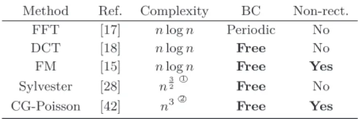
To highlight the differences between the methods, we start by comparing their algorithmic complexity, the type of admissible boundary conditions they admit, and the permissible the computational domain Ω: see Table 1. Algorithmic complexity is an indicator for the speed of a solver, while the admissible boundary conditions and the handling of non-rectangular domains influence its accuracy. The ability to handle non-rectangular domains improves also its computational efficiency.
The findings in Table 1 already indicate the potential usefulness of a mixture of FM and
CG-Table 1 Comparison of five existing fast and accurate surface normal integration methods based on three criteria: their algorithmic complexity w.r.t. the number n of pixels inside the computational domain Ω (the lower the better), the type of boundary condition (BC) they use (free boundaries are expected to reduce bias), and the permitted shape of Ω (handling non-rectangular domains can be important for accuracy and algorithmic speed)
Method Ref. Complexity BC Non-rect. FFT [17] nlog n Periodic No DCT [18] nlog n Free No FM [15] nlog n Free Yes
Sylvester [28] n32 1 ¥ Free No CG-Poisson [42] n3¥2 Free Yes 1
¥Assuming Ω is square. For rectangular domains of size nr× nc, the
complexity is O(n3 c).
2
¥Without using preconditioning techniques.
Poisson approaches as both are free of constraints in the last two criteria and so their combination may lead to a reasonably computationally efficient Poisson solver. Although other methods have their strengths in algorithmic complexity and in the application of boundary conditions (apart from FFT), we see that the flexible handling of domains is a fundamental task and a key requirement of an ideal solver for surface normal integration.
3.2 Stopping criterion for CG-Poisson
Amongst the considered methods, the Poisson solver (conjugate gradient method), where solving the discrete Poisson equation Eq. (7) corresponds to a linear system Ax = b, is the only iterative scheme. As indicated in Section 2.3, a practical solution can be reached quickly after a small number k of iterations, but k cannot be predicted exactly. The general stopping criterion for an iterative method can be based on the relative residual (ëb − Axë)/ëbë which we analyse in this paragraph.
To guarantee the efficiency of the CG-Poisson solver it is necessary to define the number k of iterations depending on the quality of the reconstruction in the iterative process. To tackle this issue we compared the MSE¥3 and the relative
residual during each CG iteration. As the solution of the linear system Eq. (14) is not unique, an additive ambiguity v Ô→ v + c, c ∈ R in the integration problem (c is the “integration constant”) occurs. Therefore, in each numerical experiment we chose the additive constant c which minimises the MSE, for fair comparison. To determine a proper relative residual, we considered the datasets “Lena”, “Peaks”, “Phantom”, “Sombrero”, and “Vase” on rectangular and non-rectangular domains. All test cases showed results similar to the graphs in Fig. 1 for the reconstruction of the “Sombrero” surface (see Fig. 2).
In this experiment the iterative solver CG-Poisson was stopped when the relative residual was lower than 10−6. However, it can be seen clearly that after
around iteration 250, the quality measured by the MSE cannot be improved and therefore using more than 400 iterations is redundant. This numerical steady state of the MSE and therefore of the residual occurs when the relative residual is between 10−3
3
¥The mean squared error (MSE) is used to quantify the error of the reconstruction. We employed it to estimate the amount of the error contained in the reconstruction compared to the original.
Fig. 1 MSE vs. relative residual during CG iterations, for the “Sombrero” dataset. Although arbitrary relative accuracy can be reached, it is not useful to go beyond a 10−3 residual, since
such refinements have very small impact on the quality of the reconstruction, as shown by the MSE graph. Similar results were obtained for all datasets used in this paper. Hence, we set as stopping criterion a 10−4relative residual, which can be considered as “safe”.
Fig. 2 “Sombrero” surface (256 × 256) used in this experiment, whose gradient can be calculated analytically. Note that the depth values are periodic on the boundaries.
and 10−4, so we use the suitable and “safe” stopping
criterion of 10−4 in subsequent experiments.
3.3 Accuracy of the solvers
First we analyse the general quality of the methods listed in Table 1 for the “Sombrero” dataset over a domain of size 256×256. In this example the gradient can be calculated analytically and furthermore the boundary conditions are periodic. Table 1 makes it obvious that all methods have no restrictions and consequently no discrimination.
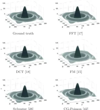
Basically all methods provide a satisfactory reconstruction, and only FM produces a less accurate solution: see Figs. 3 and 4. This can be seen more easily in Table 2, where the values of the measurements¥1 of MSE and SSIM and the
CPU time (in second) are given. The accuracy of all methods is similar, although the solution for FM, with 1.16 for MSE and 0.98 for SSIM, is slightly worse.In contrast the CPU time varies strongly, and
1
¥We tested the two common measurements MSE and SSIM. A superior reconstruction has value closer to zero for MSE and a value closer to one for SSIM. The structural similarity (SSIM) index is a method for predicting the perceived quality of an image, see Ref. [52].
Ground truth FFT [17]
DCT [18] FM [15]
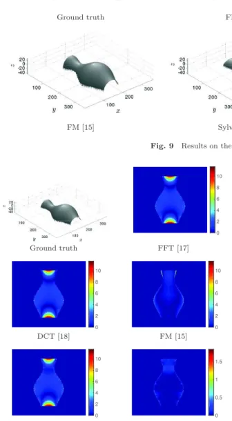
Sylvester [28] CG-Poisson [42] Fig. 3 Results on the “Sombrero” dataset (cf. Table 2).
0 0.5 1 Ground truth FFT [17] 0 0.5 1 0 0.5 1 1.5 2 2.5 DCT [18] FM [15] 0 0.02 0.04 0.06 0.08 0 0.02 0.04 0.06 0.08 Sylvester [28] CG-Poisson [42] Fig. 4 Absolute errors for the “Sombrero” dataset between the ground truth and the numerical result of each method; see Table 2. Note the different scales of the plots. To highlight the differences between all methods we use three different scales. The absolute error map of FM has its own scale due to the fact that the MSE and the maximum error differ compared to the other methods. For FFT and DCT, Sylvester and CG respectively, which have similar values for the MSE and the maximum error, we used the same scale to point out the differences.
Table 2 Results on the “Sombrero” dataset (256 × 256). As expected, all methods provide reasonably accurate solutions. However, the FM result is slightly less accurate: this is due to error accumulation by the local nature of FM, while the other methods are
global. The reconstructed surfaces are shown in Fig. 3
Method MSE (px) SSIM CPU (s) FFT [17] 0.01 1.00 <0.01
DCT [18] 0.04 1.00 0.01 FM [15] 1.00 0.98 0.07 Sylvester [28] 1.8 × 10⁻⁴ 1.00 0.18
CG-Poisson [42] 4.6× 10⁻⁵ 1.00 1.06
in this case FFT and DCT, which need around 0.01 s, are unbeatable. The time for FM and Sylvester is in a reasonable range, and only the standard CG-Poisson taking around 1.06 s being too slow and inefficient. For problems of surface reconstruction under these conditions, the choice of a solver is fairly easy: the frequency domain methods FFT and DCT are best.
3.4 Influence of boundary conditions
The handling of boundary conditions is a necessary issue which cannot be ignored. As we will show, different boundary conditions lead to surface reconstructions of different accuracy. The assumption of Dirichlet, periodic or homogeneous Neumann boundary conditions is often not justified and may even be unrealistic in some applications. A better choice is to use “natural” boundary conditions [2] of Neumann type.
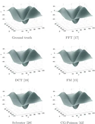
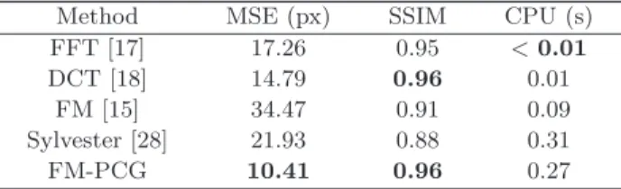
The behaviour of the discussed solvers for unjustified boundary conditions, particularly for FFT, is illustrated by the “Peaks” dataset in Figs. 5 and 6 and the associated Table 3. Almost all methods provide good reconstructions; the FM result is also acceptable. Only FFT, with 7.19 for MSE and 0.96 for SSIM, is strongly inferior and unusable for this real surface, as its accuracy is too low.
Our results show that FFT-based methods enforcing periodic boundary conditions can be discarded from the list of candidates for an ideal
Table 3 Results on the “Peaks” dataset (128 × 128). Methods enforcing periodic BC fail to provide a good reconstruction. The reconstructed surfaces are shown in Fig. 5
Method MSE (px) SSIM CPU (s) FFT [17] 7.19 0.96 <0.01 DCT [18] 0.09 1.00 <0.01 FM [15] 0.80 0.99 0.03 Sylvester [28] 0.02 1.00 0.05 CG-Poisson [42] 0.02 1.00 0.29 Ground truth FFT [17] DCT [18] FM [15] Sylvester [28] CG-Poisson [42] Fig. 5 Results on the “Peaks” dataset (see Table 3).
solver. Once again CG-Poisson is a very accurate integrator, but DCT and Sylvester are much faster and provide useful results. However, we may point out again in advance that enforcing the domain Ω to be rectangular may lead to difficulties w.r.t. the transition from foreground to background of an object.
3.5 Influence of noisy data
A key point in many applications is the question of the influence of noise on the quality of the reconstructions provided by different methods. Usually, the correctness of the given data, without noise, cannot be guaranteed. Therefore, it is essential to have a robust surface normal integrator with respect to noisy data.
To study the influence of noise, we should consider a dataset which, apart from noise, is perfect. Based on this aspect, a very reasonable test example is the “Sombrero” dataset; see Fig. 2. The advantage of “Sombrero” is that the gradient of this object is known analytically, not just approximately. Furthermore, the computational domain Ω is rectangular and the boundary conditions are periodic. For this test we added Gaussian noise with a standard deviation σ varying from 0% to 20%
0 2 4 6 8 Ground truth FFT [17] 0 0.2 0.4 0.6 0.8 0 0.5 1 1.5 2 2.5 DCT [18] FM [15] 0 0.2 0.4 0.6 0.8 0 0.2 0.4 0.6 0.8 Sylvester [28] CG-Poisson [42] Fig. 6 Absolute errors for the “Peaks” dataset between the ground truth and the numerical result of each method; see Table 3. Note the different scales of the plots. To highlight the differences between all methods we consider three different scales. The absolute error maps of FFT and FM have their own scales due to the fact that the MSE and the maximum error are very different in contrast to the other methods. For DCT, Sylvester, and CG, which have similar values for the MSE and the maximum error, we used the same scale to point out the differences.
of ë[p, q]Të
∞ to the known gradients¥1.
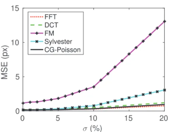
The graph in Fig. 7, which compares the MSE versus the standard deviation of Gaussian noise, indicates the robustness of the tested methods. The best performance is achieved by FFT, DCT, and CG-Poisson, even for strong noisy data with a standard deviation of 20%.
The results of Sylvester are similar, but the method suffers from weaknesses in examples with noise of higher standard deviation, i.e., larger than 10%.
As the FM integrator accumulates errors during front propagation, we observe, as expected, for highly noisy data this integrator is no longer a useful choice.
To conclude, if the accuracy of the given data is not known then FFT, DCT, and CG-Poisson are the safest integrators.
1
¥In the context of photometric stereo, it would be more realistic to add noise to the input images rather than to the gradients [53]. Nevertheless, evaluating the robustness of integrators given noisy gradients remains useful in order to compare their intrinsic properties. 0 5 10 15 20 σ (%) 0 5 10 15 MSE (px) FFT DCT FM Sylvester CG-Poisson
Fig. 7 MSE as a function of the standard deviation of a Gaussian noise, expressed as percentage of the maximal amplitude of the gradient, added to the gradient. FFT, DCT, and CG-Poisson methods provide the best results for different levels of Gaussian noise. The Sylvester method leads to reasonable results for a noise level lower than 10%. Since the FM approach propagates information in a single pass, it obviously also propagates errors, resulting in reduced robustness compared to all other approaches.
3.6 Handling non-rectangular domains
In this experiment we consider the situation when the gradient values are only known on a non-rectangular part of the grid. Applying methods needing rectangular grids [17, 18, 28] requires empirically fixing the values [p, q] := [0, 0] outside Ω (see Fig. 8), inducing a bias.
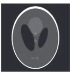
This can be explained as follows: filling the gradient with null values outside Ω creates discontinuities between the foreground and background, preventing one from obtaining reasonable results, since all solvers considered here are intended to reconstruct smooth surfaces. This problem is illustrated in Figs. 9 and 10 for the “Vase” dataset; Table 4 gives corresponding values for MSE and SSIM.
The methods can be classified into two groups. In contrast to FM and CG-Poisson, FFT, DCT, and Sylvester methods, which cannot handle flexible
Fig. 8 Mask for the “Vase” dataset. The gradient values are only known on a non-rectangular part Ω of the grid, represented by the white region. The FM and the CG-Poisson integrators can handle easily any form of domain Ω. In contrast FFT, DCT, and Sylvester rely on a rectangular domain and therefore the values [p, q] := [0, 0] need to be fixed outside Ω, in the black region.
Ground truth FFT [17] DCT [18]
FM [15] Sylvester [28] CG-Poisson [42]
Fig. 9 Results on the “Vase” dataset; see Table 4.
0 2 4 6 8 10 Ground truth FFT [17] 0 2 4 6 8 10 0 2 4 6 8 10 DCT [18] FM [15] 0 2 4 6 8 10 0 0.5 1 1.5 Sylvester [28] CG-Poisson [42] Fig. 10 Absolute errors for the “Vase” dataset between the ground truth and the numerical result of each method; see Table 4. Note the different scales of the plots. To highlight the differences between all methods we use two different scales. The absolute error maps of FFT, DCT, Sylvester, and FM have the same scale due as their maximum errors are very close. For CG we use a different scale to point out the differences.
domains, provide inaccurate reconstructions which are not useful. The non-applicability of these methods is a considerable problem, since real-world input images for 3D reconstruction are typically located within a photographed scene. This requires the flexibility to tackle non-rectangular
Table 4 Results on the “Vase” dataset (320 × 320). Methods dedicated to rectangular domains are clearly biased if Ω is not rectangular. The corresponding reconstructed surfaces are shown in Fig. 9
Method MSE (px) SSIM CPU (s) FFT [17] 5.71 0.99 0.01
DCT [18] 5.69 0.99 0.02 FM [15] 0.71 1.00 0.15 Sylvester [28] 5.99 0.98 0.36 CG-Poisson [42] 0.01 1.00 0.52
domains, while providing accurate (and efficient) reconstruction.
This experiment shows that all methods except FM and CG-Poisson are not applicable as an ideal, high-quality normal integrator for many applications.
Let us note that we also have shown that FM and CG-Poisson have complementary properties and disadvantages: the former is fast but inaccurate, and the latter is slow but accurate. This clearly motivates the combination of FM as initialisation, and a Krylov-based Poisson solver: these should combine to give a fast and accurate solver.
3.7 Summary of the evaluation
In the previous experiments we tested different scenarios which arise in real-world applications. It was found that boundary conditions and noisy data may have a strong effect on 3D reconstruction. If rectangular domains can be considered, the DCT method seems to be a realistic choice of a normal integrator followed by Sylvester and CG-Poisson.
In fact the first is unbeatably fast. However, the importance of handling non-rectangular domains, which is a practical issue in many industrial applications, cannot be underestimated. This situation leads to inaccuracies in the reconstructions of DCT and Sylvester methods. In this context FM and CG-Poisson methods achieve better results.
One can observe a certain lack of robustness w.r.t. noise of the FM integrator, especially along directions not aligned with the grid structure: see also the results in Ref. [29]. This is because of the causality concept behind the FM scheme; errors that once appear are transported over the computational domain. This is not the case using Poisson reconstruction, which is a global approach and includes a regularising mechanism via the underlying least squares model.
Due to the possibly non-rectangular nature of the domains we aim to tackle, we cannot use fast Poisson solvers as, e.g., in Ref. [18] to solve the discrete Poisson equations numerically. Instead, we explicitly construct linear systems and solve them using the CG solver as often done by practitioners. Nevertheless, the unmodified CG-Poisson solver is still quite inefficient.
4
Accelerating CG-Poisson
Let us now demonstrate the advantages of the proposed FM-PCG approach compared to other state-of-the-art methods. In doing so, we give a careful evaluation of all the components of our novel algorithm.
4.1 Preconditioned CG-Poisson
In a first step we analyse the behaviour of the CG solver when applying an additional preconditioner intended to improve the condition number and convergence speed w.r.t. the number k of iterations, thus reducing time to reach the stopping criterion.
As examples of actual preconditioners, we examined¥1 IC(τ ) and MIC(τ, α) for the test dataset
“Phantom” (see Fig. 11) for different input sizes. It was observed that MIC(τ, α∗) beats IC(τ ) if we
used α∗ = 10−3 for the global diagonal shift¥2. In 1
¥As pivot breakdowns for MIC(τ ) are possible, we considered the shifted MIC version MIC(τ, α). All methods are predefined functions in MATLAB.
2
¥This is an experimentally determined value.
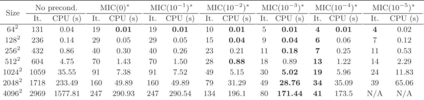
Fig. 11 “Phantom” image used in this experiment. Its gradient is unknown, so we approximate it numerically by first-order forward differences. We used this dataset for comparing preconditioners, for different image sizes, from 64 × 64 to 4096 × 4096.
the following, for simplicity we write MIC(τ )∗
for MIC(τ, α∗
)¥3. The results for MIC(0)∗
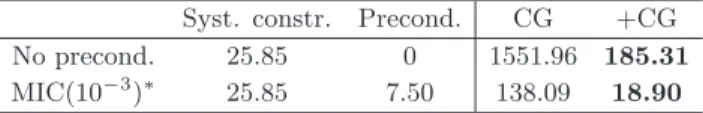
, without a fill-in strategy, are shown in Table 5 (third column) and demonstrate its usefulness compared to the non-preconditioned CG-Poisson (second column). By using MIC(0)∗
we save many iterations, greatly reducing the time taken: for example one can save around 2700 iterations and thus more than 1250 s for an image of size 4096 × 4096.
Now we show how useful a fill-in strategy can be. In columns four to eight we tested different fill-in strategies from MIC(10−1)∗
to MIC(10−5)∗
. A closer examination of Table 5 shows that MIC(10−3)∗
provides the best balance between the time needed to compute the preconditioner and the time needed to apply PCG. As an example, again for the image of size 4096 × 4096, we can reduce the number of iterations from 247 to 80, taking around 170 s instead of 290 s.
Thus, the application of preconditioning, here shifted MIC, seems to be useful in accelerating the CG-Poisson integrator, but it is not sufficient to be competitive with common fast methods. However, we will see that with proper initialisation, this standard preconditioner can already be considered to be as efficient.
4.2 Appropriate initialisation
The suggested preconditioned CG-Poisson (PCG-Poisson) method is not widely known in computer vision, although this practical method is surely not new and commonly used in numerical computing. However, we propose a novel scheme for the surface normal integration (SNI) task, using an appropriate
3
¥If the value τ in MIC(τ )∗tends to zero then the preconditioned
matrix is more dense, with more non-zero elements. As a consequence, the preconditioner is better; however it costs more time to compute the preconditioner itself.