To link to this article : DOI:10.1017/jfm.2016.470 URL : http://dx.doi.org/10.1017/jfm.2016.470
O
pen
A
rchive
T
OULOUSE
A
rchive
O
uverte (
OATAO
)
OATAO is an open access repository that collects the work of Toulouse researchers and makes it freely available over the web where possible.This is an author-deposited version published in : http://oatao.univ-toulouse.fr/
Eprints ID : 16090
To cite this version : Hwang, Yongyun and Willis, Ashley P. and Cossu, Carlo Invariant solutions of minimal large-scale structures in turbulent channel flow for Reτ up to 1000. (2016) Journal of Fluid Mechanics, vol. 802. pp. R1-1-R1-13. ISSN 0022-1120
Any correspondence concerning this service should be sent to the repository administrator: [email protected]
Invariant solutions of minimal large-scale
structures in turbulent channel flow for Re
τup to 1000
Yongyun Hwang1,†, Ashley P. Willis2 and Carlo Cossu3
1Department of Aeronautics, Imperial College London, South Kensington, London SW7 2AZ, UK 2School of Mathematics and Statistics, University of Sheffield, Sheffield S3 7RH, UK
3Institut de Mécanique des Fluides de Toulouse (IMFT), CNRS Université de Toulouse,
Allée du Pr. Camille Soula, F-31400 Toulouse, France
Understanding the origin of large-scale structures in high-Reynolds-number wall turbulence has been a central issue over a number of years. Recently, Rawat et al. (J. Fluid Mech., vol. 782, 2015, pp. 515–540) have computed invariant solutions for the large-scale structures in turbulent Couette flow at Reτ ≃128 using
an overdamped large-eddy simulation with the Smagorinsky model to account for the effect of the surrounding small-scale motions. Here, we extend this approach to Reynolds numbers an order of magnitude higher in turbulent channel flow, towards the regime where the large-scale structures in the form of very-large-scale motions (long streaky motions) and large-scale motions (short vortical structures) emerge energetically. We demonstrate that a set of invariant solutions can be computed from simulations of the self-sustaining large-scale structures in the minimal unit (domain of size Lx=3.0h streamwise and Lz=1.5h spanwise) with midplane reflection symmetry
at least up to Reτ ≃ 1000. By approximating the surrounding small scales with
an artificially elevated Smagorinsky constant, a set of equilibrium states are found, labelled upper- and lower-branch according to their associated drag. It is shown that the upper-branch equilibrium state is a reasonable proxy for the spatial structure and the turbulent statistics of the self-sustaining large-scale structures.
Key words:low-dimensional models, nonlinear dynamical systems, turbulent boundary layers
1. Introduction
The discovery of very-large-scale motions (VLSMs) has attracted significant interest in research into wall-bounded turbulence over the past decade (e.g. Hutchins & Marusic 2007). The VLSM features as a long streaky motion of streamwise turbulent
kinetic energy in the outer region, and it is typically very energetic at sufficiently high Reynolds numbers (Reτ & O(103) where Reτ is the friction Reynolds number).
It was initially proposed that this long streaky structure may be formed by the concatenation of the large-scale vortical structures, known as the large-scale motions (LSMs) (Kovasznay, Kibens & Blackwelder 1970), which themselves were speculated to be formed by merger and/or growth of near-wall hairpin vortices via a ‘bottom-up’ process (for further details, the reader may refer to a recent summary on this proposition by Adrian (2007)). However, there has been a growing body of recent evidence that the outer structures are largely independent of the near-wall process: for instance, disruption of the near-wall process with wall roughness affects the outer statistics very little (Flores, Jiménez & del Álamo 2007).
We have recently shown that the coherent structures in the outer region sustain themselves, even in the absence of the motions in the near-wall and logarithmic regions (Hwang & Cossu 2010b; Rawat et al. 2015). The self-sustaining outer structure is composed of two structural elements – a long streak and short quasistreamwise vortices, which respectively correspond to the VLSM and the LSMs (Hwang 2015). The self-sustaining process was also found to be almost identical to that in the near-wall region: (1) the streaky structure (VLSM) is amplified by the vortical structures (LSMs) via the lift-up effect (e.g. Cossu, Pujals & Depardon
2009; Pujals et al. 2009; Hwang & Cossu 2010a; Willis, Hwang & Cossu 2010); (2) the amplified streak undergoes a rapid meandering motion via secondary instability or transient growth (Park, Hwang & Cossu 2011); (3) the subsequent nonlinear regeneration of the streamwise vortical structures (Hwang & Bengana 2016).
The existence of a self-sustaining process at large scale in the outer region is of particular theoretical importance, because it indicates that the outer structures are probably organised around invariant solutions of the system, often referred to as ‘exact coherent structures’ (e.g. Nagata 1990; Waleffe 2001; Faisst & Eckhardt 2003; Wedin & Kerswell 2004; Hall & Sherwin 2010; Park & Graham 2016, and many others). The simplest non-trivial exact solutions of the Navier–Stokes equations are typically in the form of a stationary or travelling wave, being equilibria or relative equilibria in phase space. Together with unstable periodic and/or relative periodic orbits (e.g. Kawahara & Kida 2001), these invariant solutions have been shown to form a skeleton for solution trajectories in phase space (Gibson, Halcrow & Cvitanovic 2008; Willis, Cvitanovic & Avila 2013, 2016), and their understanding from a dynamical systems viewpoint has been at the heart of recent advancement in the understanding of bypass transition and low-Reynolds-number turbulence.
The goal of the present study is to demonstrate that such invariant solutions are also the driving mathematical mechanism of the large-scale outer structures given with the VLSMs and the LSMs in high-Reynolds-number turbulent channel flow. This task, however, has often been understood to be challenging. The principal difficulty lies in the emergence of a huge number of invariant solutions, which significantly hampers identification of which solutions are most relevant to given coherent structures of interest. Furthermore, the computation of the invariant solutions at such a high Reynolds number is often numerically very sensitive and expensive, yielding a substantial technical barrier. To bypass these difficulties, Rawat et al. (2015) and Rawat, Cossu & Rincon (2016) recently computed a set of coherent invariant solutions at Reynolds numbers up to Reτ = 128 by modelling all the smaller-scale
structures around the structure of interest via large-eddy simulations (LESs) with the Smagorinsky model. In these studies, the Smagorinsky constant Cs was taken as
a continuation parameter to replace the surrounding unsteady smaller-scale motions with an elevated eddy viscosity, as in Hwang & Cossu (2010b, 2011). Here, we extend this approach to a different regime of much higher Reynolds numbers up to Reτ ≃ 1000, at which the VLSMs and the LSMs emerge energetically in the flow
domain, and show that the invariant solutions are directly linked with the formation of the large-scale structures.
2. Numerical method
We consider a turbulent channel, with half-height h, in which x, y and z denote the streamwise, wall-normal and spanwise direction respectively. The two walls are located at y = 0 and y = 2h. We use a Navier–Stokes solver that is well documented in Bewley (2014). In this solver, the streamwise and spanwise directions are discretised using Fourier series with 2/3 dealiasing rule, whereas the wall-normal direction is discretised using second-order central difference. A set of LESs are considered with the static Smagorinsky model, as in previous studies (e.g. Hwang & Cossu 2010b,
2011; Rawat et al. 2015, 2016), i.e. ˜τij− δij/3 ˜τkk= −2νtS˜ij with νt= (Cs∆)˜ 2S˜D, where
˜· denotes the filtered quantity, Sij the strain rate tensor, Cs the Smagorinsky constant,
˜
∆ = ( ˜∆1∆˜2∆˜3)1/3 the nominal filter width, ˜S = (2 ˜SijS˜ij)1/2 the norm of the strain
rate tensor, and D = 1 − exp[−(y+/A+)3] with A+
=25 is the van Driest damping function. The Smagorinsky constant for turbulent channel flow is typically set in the range between Cs =0.05 and Cs =0.10 (e.g. Moin & Kim 1982; Härtel & Kleiser
1998). In particular, Cs = 0.05 has been shown to provide the best performance in
terms of accurate generation of first- and second-order turbulent velocity statistics (a posteriori test), while Cs = 0.10 is known for the model to provide the best
turbulent dissipation in comparison to the true value obtained in a direct numerical simulation (DNS) (a priori test) (Härtel & Kleiser 1998; Meneveau & Katz 2000). Mason & Cullen (1986) showed that the Smagorinsky constant Cs actually acts as
the filter width of the LES. Therefore, artificially increasing Cs allows one to damp
the small-scale motions without losing actual resolution of the large-scale structures, as also demonstrated in Hwang & Cossu (2010b). It is also important to note that the static Smagorinsky model prevents any energy transfer from the modelled residual stress to the resolved motions, ensuring that the resolved motions sustain themselves at the increased Cs. All the simulations in this study are performed by imposing
constant volume flux across the channel.
In the present study, computation of the invariant solutions is restricted to the minimal unit for the self-sustaining process of the outer structures in Hwang & Cossu (2010b), i.e. Lx=3.0h and Lz=1.5h where Lx and Lz are the streamwise and spanwise
domain sizes, respectively. An important benefit of the minimal unit is that it realises a low-dimensional dynamical set of coherent structures in the form of a VLSM (long outer streak) and LSMs (short outer vortices) without significant distortion of turbulent statistics (Hwang & Cossu 2010b; Rawat 2014; Hwang & Bengana 2016). Given the symmetry of turbulent statistics around the channel midplane, we will also focus on seeking invariant solutions with mirror symmetry about y = h. For this purpose, only the bottom half of the channel is solved by imposing the symmetric boundary condition at the channel midplane (i.e. ∂u/∂y = 0, v = 0 and ∂w/∂y = 0 at y = h where u, v and w are the streamwise, wall-normal and spanwise velocities, respectively). Except for this setting, all the simulation parameters, including the number of grid points, at two Reynolds numbers considered, Rem = 20 133 and Rem = 38 133, are
Simulation Rem Reτ Lx/h Ly/h Lz/h Nx× Ny× Nz Uc/Um Cs
F550 20 133 539 3.0 1.0 1.5 32 × 33 × 32 1.15 0.05
S550 20 133 584 3.0 1.0 1.5 32 × 33 × 32 1.13 0.20
F950 38 133 958 3.0 1.0 1.5 48 × 41 × 48 1.13 0.05
S950 38 133 1189 3.0 1.0 1.5 48 × 41 × 48 1.13 0.30
TABLE 1. Simulation parameters in the present study (before dealiasing). Here, Rem =
2Umh/ν where Um is the bulk velocity. Note that Um= (2/3)Ul where Ul is the centreline
velocity of the corresponding laminar flow with the same volume flux. The simulations tagged with ‘F’ indicate full simulations resolving near-wall motions, while those tagged with ‘S’ are simulations with only self-sustaining outer motions made by increasing the Smagorinsky constant Cs.
The artificially increased Cs values, by which the small-scale structures are replaced
with the eddy viscosity, but not the self-sustaining outer motions, are therefore also the same as those in these works (see the parameters of simulations S550 and S950 in table 1). Finally, it should be noted that the two sets of grid points, respectively for Rem=20 133 and Rem=38 133, in the present study are chosen such that the standard
LESs of the present study ensure good resolution for the small-scale near-wall motions (Zang 1991, see also figure 1), as in our previous studies (Hwang & Cossu 2010b,
2011). An examination of the energy spectra reveals that these numbers of grid points are also found to provide good spatial resolution for the computed invariant solutions, at least for the elevated Cs. We also note that the resolution of the invariant solution
for Rem=38 133 is finer than that in Waleffe (2001).
A reference simulation is first performed to check turbulence statistics of the half-channel LES simulation at Reτ ≃ 950, with the value Cs =0.05 (F950) known
to provide the best statistical fit to the full DNS result (Hwang & Cossu 2010b). In figure 1, its first- and second-order turbulence statistics are compared with those of full-channel LES with the same streamwise and spanwise computational domain (Hwang & Cossu 2011) as well as those of DNS by del Álamo et al. (2004) at Reτ = 934. Overall, the half-channel simulation generates fairly good turbulence
statistics compared with those from the full-channel LES, which itself shows reasonable agreement with the data from full DNS. The only appreciable difference between the half-channel and full-channel simulations appears in the wall-normal velocity fluctuation very near the channel centre, due to the symmetry condition. This indicates that the half-channel simulation does not lose important physical features, except around the very centre of the channel, where mainly dissipation of structures is expected due to the small shear in this region.
3. The invariant structures
3.1. Computation of invariant solutions
Now, we increase Cs such that the simulation contains only the large-scale
self-sustaining structures in the given computational domain (simulations S550 and S950 in table 1). By doing so, all the structures smaller than the large-scale structures are removed, while their roles are modelled with the artificially elevated eddy viscosity. It is very important to note that the removal with an appropriate increase in Cs does not
100 101 102 103 100 101 102 103 0 1 2 3 4 5 0 10 15 20 25 (a) (b)
FIGURE 1. (a) Mean velocity and (b) turbulent velocity fluctuations: ——, half-channel
simulation with Cs=0.05 (F950); - - - -, full-channel simulation with Cs=0.05 (Hwang &
Cossu 2011); – · – · –, DNS at Reτ =934 by del Álamo et al. (2004).
structures themselves, as extensively discussed in the previous studies (Hwang & Cossu 2010b; Hwang 2015; Rawat et al. 2015; Hwang & Bengana 2016). Therefore, the computed invariant solutions at the artificially elevated Cs would conceptually
represent the structures in the ‘presence of the surrounding small scales’, which is modelled by the eddy viscosity, while enabling us to compute the invariant solutions with the relatively low resolutions at the high Reynolds numbers considered. The invariant solutions of the system with the elevated Cs are sought in the subspace
satisfying the so-called shift-reflect symmetry
[u, v, w, p](x, y, z) = [u, v, −w, p](x − Lx/2, y, −z), (3.1)
where p is the pressure, together with the mirror symmetry about y = 0. It should be mentioned that this specific symmetry is intentionally posed to find the invariant solutions containing the ‘sinuous’ mode of streak instability (i.e. streak meandering motions along the streamwise direction). The sinuous mode of streak instability has been consistently found to be the dominant mechanism of the streak breakdown in our previous theoretical analysis (Park et al. 2011) as well as the minimal channel simulation for the outer structures (Hwang & Bengana 2016). Indeed, in this study, we have also found that imposing the symmetry (3.1) in the present half-channel simulation with the increased Cs (S550 and S950) does not engender any significant
difference from the simulation without this symmetry (see figure 4). It is worth mentioning that Waleffe (2001) also imposed this symmetry for computation of his invariant solutions for the same reason.
To compute the invariant solutions, we have implemented a Newton–Krylov– Hookstep method and applied it to the present LES solver. Details of the method are given in Willis et al. (2013), and it is similar to that proposed by Viswanath (2007). This method computes an invariant solution by minimising the relative error between an initial guess for an initial flow field and the same field time-stepped by an interval T and shifted in the streamwise direction by a distance −lx. For an
equilibrium state the choice of T is arbitrary, and the phase speed of the equilibrium is c = lx/T. Throughout this study, the computation of the invariant solutions is
carried out with T = 16.7h/Um. All the solutions are computed to a relative-error
0.20 0.25 0.30 0.35 0.30 0.35 0.40 0.45 0.50 400 500 600 700 800 1200 1000 1400 1600 800 (a) (b)
FIGURE 2. Bifurcation of invariant solutions with Cs: (a) Rem=20 133; (b) Rem=38 133.
Here, the simulations S550 and S950 respectively correspond to Cs = 0.2 in (a) and
Cs=0.3 in (b).
invariant solutions are expected to sit on the so-called ‘edge’ state, which refers to the phase-space boundary manifold between the basic and the chaotic states (e.g. Skufca, Yorke & Eckhardt 2006), we start by computing the edge state for the S550 simulation in the given subspace, using the standard bisection technique to obtain a good initial guess for the Newton iteration (e.g. Duguet, Willis & Kerswell 2008; Avila et al. 2013). Several instantaneous flow fields on the edge state are given for initial guess of the Newton solver, and we found an invariant solution propagating downstream with a constant speed (i.e. a travelling wave) from S550. Numerical continuation in Cs is subsequently performed, as in Rawat (2014) and Rawat et al.
(2015).
Figure 2(a) shows the bifurcation of the invariant solutions with Cs by plotting Reτ
of each of the solutions. Here, we note that Reτ in this case is given as a measure of
the friction of each solution, revealing its relevance to high-Reynolds-number flows, i.e. Reτ =2uτ/UmRem. Therefore, Reτ given here is different for each invariant solution
and represents its friction. Continuation reveals that the invariant solutions experience a saddle-node bifurcation as Cs is gradually lowered from a large value. Two invariant
solutions are found to emerge at the critical Cs (≃ 0.335), as often observed in
transitional Reynolds numbers: one has a low drag (lower-branch solution) and the other has a high drag (upper-branch solution). The solutions obtained at Rem=20 133
are further continued to a higher Reynolds number, Rem = 38 133. Essentially, the
same behaviour with Cs is obtained at this Reynolds number, as shown in figure 2(b).
3.2. Spatial structure of the invariant solutions
The computed invariant solutions are visualised in figure 3. Both of the upper-and lower-branch solutions are characterised by a ‘wavy’ streak (blue isosurfaces) and streamwise vortices on the flank (red isosurfaces), clearly reflecting their tight physical link to the self-sustaining process of the outer coherent structures, i.e. streak generation via the lift-up effect with the vortices, and sinuous-mode streak instability with nonlinear feeding of the vortices. The upper-branch solution exhibits a strongly wavy streak and intense streamwise vortices, while the lower-branch solution is composed of a relatively straight streak and weak streamwise vortices (see the levels of the red isosurfaces in figure 3). This feature is consistent with that of the invariant solutions in, e.g., Waleffe (2001). The invariant solutions here, however, are obtained
0 0.5 1.0 1.5 0 0.5 1.0 1.5 0 1 2 3 0 1 2 3 Flow Flow (a) (b)
FIGURE 3. Visualisation of the invariant solutions: (a) U950; (b) L950. In both (a) and
(b), the blue isosurfaces indicate u+ = −2.96 and the green ones ν
t = 7.2ν. The red
isosurfaces in (a) and (b) are Q+=3.6 × 10⁻⁵ and Q+=2.0 × 10⁻⁵, respectively.
0 0.2 0.4 U950 S950 and S950 with shift-reflect sym. S950 and S950 with shift-reflect sym. S950 and S950 with shift-reflect sym. S950 and S950 with shift-reflect sym. U950 U950 U950 L950 L950 L950 L950 0.6 0.8 1.0 0 0.2 0.4 0.6 0.8 1.0 0 0.2 0.4 0.6 0.8 1.0 0 0.2 0.4 0.6 0.8 1.0 1.0 0.2 0.4 0.6 0.8 1.0 0.2 0.4 0.6 0.8 10 20 30 1 2 3 4 (a) (b) (c) (d )
FIGURE 4. The normal profile of (a) mean velocity, and (b) streamwise, (c)
wall-normal and (d) spanwise velocity fluctuations: ——, S950; - - - -, the symmetry-constrained S950; – ·· – ·· –, U950; – · – · –, L950.
by modelling the surrounding small-scale structures with an eddy viscosity. The eddy viscosity is typically found to be quite strong around the streak, where high local shear is expected (the green isosurfaces in figure 3), as also found by Rawat et al. (2015,
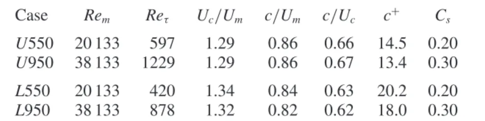
Case Rem Reτ Uc/Um c/Um c/Uc c+ Cs
U550 20 133 597 1.29 0.86 0.66 14.5 0.20 U950 38 133 1229 1.29 0.86 0.67 13.4 0.30 L550 20 133 420 1.34 0.84 0.63 20.2 0.20 L950 38 133 878 1.32 0.82 0.62 18.0 0.30
TABLE 2. Scaling of the speed of the invariant solutions. Here, c and Uc are the
propagating speed and the centreline velocity of each travelling wave solution, respectively. In the first column, U and L respectively indicate the upper- and lower-branch solutions.
kinematic viscosity because of the high Reynolds numbers considered – the maximum eddy viscosities of the upper- and the lower-branch solutions are respectively found as νt=8.48ν and νt=7.6ν, the values being an order of magnitude larger than those
in Rawat et al. (2015, 2016). This follows from the higher values of Cs and, in
particular, the much higher Reynolds numbers considered here.
Table 2 summarises the propagating speed of the computed invariant solutions with their friction velocity and centreline velocity at Rem=20 133 and Rem=38 133. The
propagating speeds of the upper- and the lower-branch solutions are respectively found to be c ≃ 0.66Uc and c ≃ 0.62Uc, and they scale more closely with their centreline
velocity Uc than with their friction velocity uτ. Although the centreline velocity Uc
of each of the invariant solutions is not the same as that from full turbulent statistics given in figure 1, this finding supports the observation by del Álamo & Jiménez (2009) and Song et al. (2016), who showed that the advection velocity of the outer structures scales with the centreline velocity. This behaviour is quite intriguing, because the single turnover time scale of self-sustaining process of outer coherent structures has been found to scale well with the friction velocity uτ (Hwang & Bengana 2016). It
is currently too early to draw any firm conclusion, but this indicates that the velocity scale of propagation of an outer structure might not be the same as the turnover time scale of the self-sustaining process.
The first- and second-order statistics of the two computed invariant solutions are compared with those of simulation S950 in figure 4. Here, the data of S950 with the shift-reflect symmetry (3.1) are plotted together. The good agreement of the statistics of simulations S950 and S950 with (3.1) suggests that the present minimal unit for the large-scale structures in the shift-reflect subspace does not greatly limit the generation of good statistics. The statistics of the upper-branch solution U950 are found to show reasonably good agreement with those of S950 roughly below y ≃ 0.4h–0.5h, despite the fact that the solution itself is a relative equilibrium, not able to fully describe the chaotic, quasiperiodic dynamics of simulation S950 (i.e. bursting (Flores & Jiménez 2010; Hwang & Bengana 2016)). We also note that the difference in statistics between an upper-branch solution and full simulation is expected. This level of difference also appears in other works that make the analogous comparison at low Reynolds numbers (e.g. Kerswell & Tutty 2007; Schneider, Eckhardt & Yorke
2007; Park & Graham 2016). As these authors indicate, this observation suggests that computation of unstable time-periodic orbits would be a more promising way to represent the dynamics of coherent structures in simulation S950 (Kawahara & Kida
2001; Gibson et al. 2008; Willis et al. 2013). Also as expected, the statistics of the lower-branch solution L950 do not show such a level of agreement – the lower-branch solution sits on the edge state of simulation S950. These results indicate that only the upper-branch solution is statistically similar to simulation S950.
10–2 10–3 0 10 20 30 10–4 10–2 10–3 10 20 30 (a) (b)
FIGURE 5. Phase portrait in the planes (a) Estreak–Evor and (b) I–D at Rem=38 133, where
Il and Dl indicate the corresponding production and dissipation of laminar flow at the same
Reynolds number. Colours: red, S950; dashed green, the symmetry-constrained S950; blue, U950; orange, L950.
Finally, the invariant solutions and the solution trajectories of simulations S950 and the symmetry-constrained S950 are projected onto the planes Estreak–Evor and I–D,
reported in figure 5. Here, Estreak and Evor respectively represent energy of the streak
and that of the streamwise vortices, and are defined by Estreak= [1/(2V)]
R V(u ′/U m)2dV and Evor = [1/(2V)] R V(v/Um) 2 + (w/U
m)2dy, where u′ is the streamwise velocity
fluctuation. I and D are respectively the energy input and dissipation of the system, defined by I = −(1/V)RVu· ∇p dV and D = −(1/V)R
Vu· (∇ · ((νT/2)(∇u + ∇u
T)))dV
with u = (u, v, w) and νT = ν + νt. We note that if E ≡ [1/(2V)]
R
V u· u dV, then
dE/dt = I − D. In the plane Estreak–Evor (figure 5a), solution trajectories for both
simulations S950 and the symmetry-constrained S950 reveal that their Estreak and
Evor are found to be slightly negatively correlated, indicating the presence of the
self-sustaining process given by the interaction between the streak and the streamwise vortices. The solution trajectories of these simulations are maintained roughly around 20Il and 20Dl in the I–D plane (figure 5b); these values are an order of magnitude
larger than those at low Reynolds numbers (e.g. Kawahara & Kida 2001; Gibson et al. 2008; Willis et al. 2013, 2016). This is essentially due to the high Reynolds number considered in the present study, which leads to the energy input to the system being substantially larger than that at low Reynolds numbers. This indicates that the role of the eddy viscosity introduced here differs from that of the molecular one, because it enables us to maintain the large energy input to the system occurring in a high-Reynolds-number flow unlike the molecular viscosity. In both the planes Estreak–Evor and I–D, the upper-branch solution U950 is found to be placed in the
middle of the turbulent trajectories of simulations S950 and the symmetry-constrained S950. The lower-branch solution L950 is almost completely separated from the trajectories, consistent with the observation on the first- and second-order statistics made with figure 4.
3.3. Bifurcation with the Reynolds number
Finally, to understand the connection between the invariant states of the Navier–Stokes equation at transitional Reynolds number and those of this study at fairly high Reynolds numbers, numerical continuation is further performed by gradually lowering
104 103
102 103
101
FIGURE 6. Bifurcation diagram of the invariant solutions in the plane Rem–Reτ:
E, Cs=0.0; u, Cs=0.30.
the Reynolds number using the computed invariant solutions with high resolution at Reτ ≃ 950 (i.e. U950 and L950). Figure 6 reports bifurcation of the invariant
solutions with the Reynolds number. The solutions for Cs=0.30 reveal a saddle-node
bifurcation at a fairly low critical Reynolds number around Rem,c ≃ 1693–1707
(Reτ ,c≃71). The Smagorinsky constant Cs is subsequently lowered around this low
Rem, such that invariant solutions of the Navier–Stokes equation are retrieved. The
exact solutions, directly linked to the large-scale structures in the minimal unit, are found to emerge approximately at Rem,c ≃ 1120 (Reτ ,c ≃ 52) via saddle-node
bifurcation. We note that this Rem,c is much lower than Rem,c≃1867 (Reτ ,c≃ 68.2)
of the invariant solutions found by Park & Graham (2016) with a similar box size, due to the different symmetry imposed in the present study (their solution P4 with Lx× Lz= πh × π/2h).
The exact solutions of the Navier–Stokes equations (Cs=0.0) are finally continued
by increasing the Reynolds number. While the upper-branch solution could not be continued for Rem & 2223, the lower-branch solution is obtained up to Rem = 8889.
Interestingly, the lower-branch solution of the Navier–Stokes equation is found to generate smaller skin friction than those solutions with elevated eddy viscosity (Cs = 0.30) on increasing the Reynolds number. However, it should be noted that
the eddy viscosity used here is designed to model all the surrounding smaller-scale structures, including the near-wall motions generating an appreciable amount of turbulent skin friction. The difference between the solutions with Cs = 0.0 and
Cs=0.30 probably originates from this nature of the eddy viscosity. 4. Concluding remarks
Invariant solutions corresponding to large-scale turbulent motions at high Reynolds numbers have been obtained following the approach of Rawat (2014) and Rawat et al. (2015, 2016), where surrounding small-scale structures are modelled with an eddy viscosity (i.e. Smagorinsky model with the artificially elevated Cs as a
continuation parameter). Here, we show that these solutions, and in particular the upper-branch solution, can be obtained at much higher Reynolds numbers (up to Reτ ≃1000), a different regime where the large-scale structures in the form of long
streaks (VLSMs) and quasistreamwise vortical structures (LSMs) emerge energetically in turbulent channel flow. This finding suggests that the large-scale structures are probably organised around these invariant solutions, providing direct evidence of their
significance at sufficiently high Reynolds numbers. This finding also tightly establishes their relation to the self-sustaining process of the large-scale structures (Hwang & Cossu 2010b; Rawat et al. 2015; Hwang & Bengana 2016), while implying that the dynamical systems approach, plus visualisation of the relevant phase space, could be used to enlighten at least some aspects of the given coherent structures at fairly high Reynolds numbers. However, the invariant solutions found here do not fully represent the dynamics occurring in real flows (i.e. bursting (Flores & Jiménez 2010; Hwang & Bengana 2016)). In this respect, extending the present approach to computation of the relative periodic orbits would be a fruitful path to follow towards more accurate modelling of the large-scale dynamics (Kawahara & Kida 2001; Willis et al. 2013,
2016). Finally, it should be mentioned that the self-sustaining energy-containing motions in wall-bounded turbulent flows at high Reynolds numbers appear in a self-similar form throughout the entire logarithmic region (Hwang & Cossu 2011; Hwang 2015), as originally hypothesised by Townsend (1976) (i.e. attached eddy hypothesis). Each of the energy-containing motions is typically characterised by its spanwise length scale (Hwang & Cossu 2011; Hwang 2015; Hwang & Bengana 2016), suggesting that the invariant solutions with different spanwise length scales may be linked to these self-similar motions. This also implies that a thorough investigation of the invariant solutions with different sets of the length scales needs to be carried out in order to clarify the relation between the ‘real’ and ‘exact’ coherent structures using a numerical experiment given in the present study. Exploring such a link between the invariant solutions and the concept of the attached eddies might unveil the nature of the self-sustaining coherent structures. This would be an important step towards a consistent theoretical description of wall-bounded shear flows in a wide range of Reynolds numbers, because the attached eddy hypothesis has provided an important theoretical basis for a consistent statistical description of high-Reynolds-number wall turbulence (e.g. Townsend 1976; Perry & Chong 1982).
Acknowledgement
Y.H. was supported by the Engineering and Physical Sciences Research Council (EPSRC) in the UK (EP/N019342/1).
References
ADRIAN, R. J. 2007 Hairpin vortex organization in wall turbulence. Phys. Fluids 19, 041301.
DEL ÁLAMO, J. C. & JIMÉNEZ, J. 2009 Estimation of turbulent convection velocities and corrections
to Taylor’s approximation. J. Fluid Mech. 640, 5–26.
DEL ÁLAMO, J. C., JIMÉNEZ, J., ZANDONADE, P. & MOSER, R. D. 2004 Scaling of the energy
spectra of turbulent channels. J. Fluid Mech. 500, 135–144.
AVILA, M., MELLIBOVSKY, F., ROLAND, N. & HOF, B. 2013 Streamwise-localized solutions at the
onset of turbulence in pipe flow. Phys. Rev. Lett. 110, 224502.
BEWLEY, T. R. 2014 Numerical Renaissance: Simulation, Optimization, and Control. Renaissance
Press.
COSSU, C., PUJALS, G. & DEPARDON, S. 2009 Optimal transient growth and very large scale structures in turbulent boundary layers. J. Fluid Mech. 619, 79–94.
DUGUET, Y., WILLIS, A. P. & KERSWELL, R. R. 2008 Transition in pipe flow: the saddle structure
on the boundary of turbulence. J. Fluid Mech. 613, 255–274.
FAISST, H. & ECKHARDT, B. 2003 Travelling waves in pipe flow. Phys. Rev. Lett. 91, 224502. FLORES, O. & JIMÉNEZ, J. 2010 Hierarchy of minimal flow units in the logarithmic layer. Phys.
FLORES, O., JIMÉNEZ, J. &DEL ÁLAMO, J. C. 2007 Vorticity organization in the outer layer of turbulent channels with disturbed walls. J. Fluid Mech. 591, 145–154.
GIBSON, J. F., HALCROW, J. & CVITANOVIC, P. 2008 Visualizing the geometry of state space in
plane Couette flow. J. Fluid Mech. 611, 107–130.
HALL, P. & SHERWIN, S. J. 2010 Streamwise vortices in shear flows: harbingers of transition and
the skeleton of coherent structures. J. Fluid Mech. 661, 178–205.
HÄRTEL, C. & KLEISER, L. 1998 Analysis and modelling of subgrid-scale motions in near-wall
turbulence. J. Fluid Mech. 356, 327–352.
HUTCHINS, N. & MARUSIC, I. 2007 Evidence of very long meandering features in the logarithmic
region of turbulent boundary layers. J. Fluid Mech. 579, 1–28.
HWANG, Y. 2015 Statistical structure of self-sustaining attached eddies in turbulent channel flow.
J. Fluid Mech. 723, 264–288.
HWANG, Y. & BENGANA, Y. 2016 Self-sustaining process of minimal attached eddies in turbulent
channel flow. J. Fluid Mech. 795, 708–738.
HWANG, Y. & COSSU, C. 2010a Linear non-normal energy amplification of harmonic and stochastic
forcing in the turbulent channel flow. J. Fluid Mech. 664, 51–73.
HWANG, Y. & COSSU, C. 2010b Self-sustained process at large scales in turbulent channel flow.
Phys. Rev. Lett. 105, 044505.
HWANG, Y. & COSSU, C. 2011 Self-sustained processes in the logarithmic layer of turbulent channel
flows. Phys. Fluids 23, 061702.
KAWAHARA, G. & KIDA, S. 2001 Periodic motion embedded in plane Couette turbulence: regeneration
cycle and burst. J. Fluid Mech. 449, 291–300.
KERSWELL, R. R. & TUTTY, O. R. 2007 Recurrence of travelling waves in transitional pipe flow.
J. Fluid Mech. 584, 69–102.
KOVASZNAY, L. S. G., KIBENS, V. & BLACKWELDER, R. F. 1970 Large-scale motion in the
intermittent region of a turbulent boundary layer. J. Fluid Mech. 41, 283–325.
MASON, P. J. & CULLEN, N. J. 1986 On the magnitude of the subgrid-scale eddy coefficient in large-eddy simulations of turbulent channel flow. J. Fluid Mech. 162, 439–462.
MENEVEAU, C. & KATZ, J. 2000 Scale-invariance and turbulence models for large-eddy simulation.
Annu. Rev. Fluid. Mech. 32, 1–32.
MOIN, P. & KIM, J. 1982 Numerical investigation of turbulent channel flow. J. Fluid Mech. 118, 341–377.
NAGATA, M. 1990 Three-dimensional finite-amplitude solutions in plane Couette flow: bifurcation
from infinity. J. Fluid Mech. 217, 519–527.
PARK, J., HWANG, Y. & COSSU, C. 2011 On the stability of large-scale streaks in the turbulent
Couette and Poiseuille flows. C. R. Mèc. 339 (1), 1–5.
PARK, J. S. & GRAHAM, M. D. 2016 Exact coherent states and connections to turbulent dynamics
in minimal channel flow. J. Fluid Mech. 782, 430–454.
PERRY, A. E. & CHONG, M. S. 1982 On the mechanism of turbulence. J. Fluid Mech. 119, 173–217.
PUJALS, G., GARCÍA-VILLALBA, M., COSSU, C. & DEPARDON, S. 2009 A note on optimal transient
growth in turbulent channel flows. Phys. Fluids 21, 015109.
RAWAT, S. 2014 Coherent dynamics of large-scale turbulent motions. PhD thesis, Université de
Toulouse, http://ethesis.inp-toulouse.fr/archive/00003011.
RAWAT, S., COSSU, C., HWANG, Y. & RINCON, F. 2015 On the self-sustained nature of large-scale motions in turbulent Couette flow. J. Fluid Mech. 782, 515–540.
RAWAT, S., COSSU, C. & RINCON, F. 2016 Travelling-wave solutions bifurcating from relative periodic
orbits in plane Poiseuille flow. C. R. Méc. 344, 448–455.
SCHNEIDER, T. M., ECKHARDT, B. & YORKE, J. A. 2007 Turbulence transition and the edge of
chaos in pipe flow. Phys. Rev. Lett. 99, 034502.
SKUFCA, J. D., YORKE, J. A. & ECKHARDT, B. 2006 Edge of chaos in a parallel shear flow. Phys.
Rev. Lett. 96 (17), 174101.
SONG, B., BARKLEY, D., HOF, B. & AVILA, M. 2016 Speed and structure of turbulent fronts in
pipe flow. arXiv:1603.04077.
VISWANATH, D. 2007 Recurrent motions within plane Couette turbulence. J. Fluid Mech. 580, 339–358.
WALEFFE, F. 2001 Exact coherent structures in channel flow. J. Fluid Mech. 435, 93–102.
WEDIN, H. & KERSWELL, R. R. 2004 Exact coherent structures in pipe flow: travelling wave
solutions. J. Fluid Mech. 508, 333–371.
WILLIS, A. P., CVITANOVIC, P. & AVILA, M. 2013 Revealing the state space of turbulent pipe flow
by symmetry reduction. J. Fluid Mech. 721, 514–540.
WILLIS, A. P., CVITANOVIC, P. & AVILA, M. 2016 Symmetry reduction in high dimensions, illustrated
in a turbulent pipe. Phys. Rev. E 93, 022204.
WILLIS, A. P., HWANG, Y. & COSSU, C. 2010 Optimally amplified large-scale streaks and drag
reduction in the turbulent pipe flow. Phys. Rev. E 82, 036321.
ZANG, T. A. 1991 Numerical simulation of the dynamics of turbulent boundary layers: perspectives