Deep learning with multiple modalities : making the most out of available data

(1)

Deep learning with multiple modalities : making the

most out of available data

Mémoire

Sébastien De Blois

Maîtrise en génie électrique - avec mémoire

Maître ès sciences (M. Sc.)

(2)

Deep learning with multiple modalities : making the

most out of available data

Mémoire

Sébastien de Blois

Sous la direction de:

(3)

Résumé

L’apprentissage profond, un sous domaine de l’apprentissage machine, est reconnu pour nécessiter une très grande quantité de données pour atteindre des performances satisfaisantes en généralisation. Une autre restriction actuelle des systèmes utilisant l’apprentissage machine en lien avec les données est la nécessité d’avoir accès au même type de données autant durant la phase d’entrainement du modèle que durant la phase de test de celui-ci. Dans plusieurs cas, ceci rend inutilisable en entrainement des données de modalité supplémentaire pouvant possiblement apporter de l’information additionnelle au système et l’améliorer. Dans ce mémoire, plusieurs méthodes d’entrainement permettant de tirer avantage de modalités additionnelles disponibles dans des jeux de données seulement en entrainement et non durant la phase de test seront proposées. Pour débuter, nous nous intéressons à diminuer le bruit présent dans images.. On débute le mémoire avec la technique la plus simple, soit un débruitage avant une tâche pour augmenter la capacité du système à faire cette tâche. Par la suite, deux techniques un peu plus poussées proposant de faire un débruitage guidé pour augmenter les performances d’une tâche subséquente sont présentées. On conclut finalement cette thèse en présentant une technique du nom d’Input Dropout permettant d’utiliser très facilement une modalité seulement disponible en entrainement pour augmenter les performances d’un système, et ce pour une multitude de tâches variées de vision numérique.

(4)

Abstract

Deep learning, a sub-domain of machine learning, is known to require a very large amount of data to achieve satisfactory performance in generalization. Another current limitation of these machine learning systems is the need to have access to the same type of data during the training phase of the model as during its testing phase. In many cases, this renders unusable training on additional modality data that could possibly bring additional information to the system and improve it. In this thesis, several training methods will be proposed to take advantage of additional modalities available in datasets only in training and not in testing. We will be particularly interested in reducing the noise present in images. The thesis begins with the simplest technique, which is a denoising before a task to increase the system’s ability to perform a task. Then, two more advanced techniques are presented, which propose guided denoising to increase the performance of a subsequent task. Finally, we conclude this thesis by presenting a technique called Input Dropout that facilitates the use of modality only available in training to increase the performance of a system, and this for a multitude of varied computer vision tasks.

(5)

List of Tables

1.1 Thermal only vs all noises on the test set: Accuracy, Sensitivity, Specificity and D-C. 12

1.2 All noises vs thermal noise: detection accuracy . . . 12

1.3 S-T vs S-T* with 250 images: Accuracy, Sensitivity, Specificity and D-C. . . 17

1.4 Denoising vs no-denoising: sensitivity and D-C . . . 17

1.5 Results of denoising vs no-denoising: detection accuracy . . . 18

1.6 Denoising vs no-denoising: Blobaccuracyand Blobrecall . . . 18

1.7 S-TS vs S-TS*: Accuracy, Sensitivity, Specificity and D-C. . . 19

1.8 CycleGAN vs End2End: Accuracy, Sensitivity, Specificity and D-C. . . 22

1.9 Conventional denoising: sensitivity and D-C . . . 25

1.10 Conventional denoising: detection accuracy . . . 25

1.11 DL 250 vs Wavelet BayesShrink: Blobaccuracyand Blobrecall . . . 25

2.1 Results of the dehazing model on the NYU depth foggy dataset in comparison to the literature: PSNR and SSIM . . . 34

2.2 Results on the test set with SEG-NET segmentation on foggy Cityscape: PSNR and SSIM 37 2.3 Results on the test set with DeepLabv3 segmentation on foggy Cityscape: IoU, iIoU and RHA . . . 38

2.4 Results on the test set with U-NET segmentation on foggy Cityscape: IoU . . . 38

2.5 Results on the test set with SEG-NET segmentation (foggy Cityscape) for hypothesis 1 of fine-tuning: RHA and IoU . . . 41

2.6 Results on the test set with SEG-NET segmentation (foggy Cityscape) for hypothesis 2 of fine-tuning: RHA and IoU . . . 42

2.7 Results on the test set with SEG-NET segmentation (foggy Cityscape) for hypothesis 2 of fine-tuning with anti-forgetting: RHA and IoU . . . 42

2.8 Results on the test set for segmentation after dehazing: IoU . . . 44

2.9 Results of DFD on the test set with DEPTH-NET with D-Hazy dataset . . . 46

2.10 Results for tests of denoising for segmentation with radar signals: Accuracy, sensitivity, specificity and D-C . . . 48

2.11 Results for tests of denoising for segmentation with radar signals: detection accuracy 49 2.12 Denoising for segmentation with radar signals: Blobaccuracyand Blobrecall. . . 50

2.13 Results on dehazing with NYU: Standard dehazing vs DFD vs MTL V1 vs MTL V2 56 2.14 Results on depth prediction with NYU: Standard dehazing vs DFD vs End2End vs MTL V1 vs MTL V2 . . . 56

2.15 Results on dehazing with Foggy Cityscape: Standard dehazing vs MTL V1 vs MTL V2 vs dehazing for segmentation . . . 57

2.16 Results on segmentation with Foggy Cityscape: Standard dehazing vs MTL V1 vs MTL V2 vs dehazing for segmentation . . . 58

(8)

2.17 MTL with 250 samples vs End2End vs Denoising vs Denoising4Seg: Blobaccuracy and

Blobrecall . . . 61

2.18 MTL with 5000 samplesvs End2End vs Denoising4Seg: Blobaccuracyand Blobrecall. . . 61

3.1 Quantitative results for single image dehazing using an additional depth (RGB+D) and segmentation (RGB+S) modality at training time . . . 72

3.2 Classification accuracies RGB+D . . . 74

3.3 Tracking error in translation and rotation . . . 76

3.4 Mean average precision (mAP) with an IoU of 0.5 results with RGB+T for nighttime and daytime pedestrian detection . . . 77

3.5 Results for tests of Input Dropout with radar signals for sensitivity and DC . . . 79

3.6 Results for tests of denoising for segmentation with radar signals . . . 79

3.7 Denoising for segmentation with radar signals for Blobaccuracyand Blobrecall . . . 80

3.8 Quantitative results for dehazing with RGB+D with and without Network Dropout at training time, RGB-only at test time. . . 81

(9)

List of Figures

1.1 The sea clutter problem . . . 6

1.2 Illustration of sensitivity and specificity . . . 8

1.3 Illustration of the calculation of the dice coefficient . . . 9

1.4 Recall vs accuracy compromise, example . . . 11

1.5 Image-to-Image translation with conditional adversarial networks. . . 13

1.6 U-net architecture . . . 14

1.7 Proposed denoising+segmentation/detection model scheme . . . 15

1.8 Samples for denoising . . . 17

1.9 Recall vs Accuracy compromise for 250 images with denoising . . . 18

1.10 Structure of the classic CycleGAN . . . 20

1.11 Samples for denoising radar images using CycleGAN . . . 21

1.12 Samples for denoising radar images using CycleGAN showing the differences in the outputs . . . 22

1.13 Samples for denoising with conventional method . . . 24

1.14 Recall vs accuracy compromise for denoising DL or Wavelet BayesShrink . . . 26

1.15 Samples for segmentation of denoising conventional vs deep learning methods . . . . 26

1.16 Why pre-denoising improves the situation. . . 27

2.1 DFS model . . . 33

2.2 Qualitative examples for haze removal of images from the D-Hazy dataset . . . 35

2.3 Two examples showing the performance of the proposed DFS technique . . . 39

2.4 Two other examples showing the performance of the proposed DFS technique . . . . 40

2.5 Training procedure for the SAD technique . . . 43

2.6 Depth prediction of RGB images hazy vs non-hazy . . . 45

2.7 DFD model . . . 46

2.8 Qualitative examples for depth prediction of RGB images from the D-Hazy dataset . . 47

2.9 DFS model with radar signals. . . 48

2.10 Samples for denoising for segmentation with radar signals . . . 49

2.11 Recall vs accuracy compromise for 2500 samples with denoising for segmentation with radar signals . . . 50

2.12 Multitask with GAN for Image-to-Image translation Version 1 . . . 53

2.13 Multitask with GAN for Image-to-Image translation Version 2 . . . 54

2.14 Qualitative examples for depth prediction of RGB images from the D-Hazy dataset, MTL V2 vs End2End . . . 57

2.15 Qualitative examples for segmentation of RGB images from the D-Hazy dataset using DFS and MTL . . . 59

(10)

2.16 Multitask with GAN for Image-to-Image translation Version 2 adapted for the radar

problem . . . 60

2.17 Recall vs accuracy compromise for 250 samples with MTL . . . 61

2.18 Recall vs accuracy compromise for 5000 samples with MTL . . . 62

2.19 Denoising for something versus multitask learning . . . 63

3.1 Input Dropout strategy . . . 68

3.2 Network Dropoutstrategy . . . 70

3.3 Schema of GAN for missing modality . . . 71

3.4 Qualitative examples for dehazing RGB images from the D-Hazy dataset with Input Dropout . . . 73

3.5 Qualitative examples for dehazing RGB images from the Foggy Cityscapes with Input Dropout . . . 73

3.6 Modality Distillation setup . . . 75

3.7 Examples of RGB and depth frames from the NYUD (RGB-D) dataset. . . 75

3.8 Qualitative examples for pedestrian detection . . . 78

3.9 Samples for Input Dropout with radar signals . . . 80

3.10 Input Dropout for sensor loss: RGB+T . . . 84

3.11 Input Dropout for sensor loss: RGB+D . . . 84 3.12 Toy network architecture used for derivation of ModDrop regularization properties . 85

(11)

(12)

"To invent is to think on the side." Unknown

(13)

Foreword

The work covered in this thesis was carried out as part of a project with Thales, I would like to thank all the people at Thales who have helped me in any way they could, a special thanks to Rana Farah, Vincent Meslot, Dominique Perron and Marlene Gauthier.

I would like to thank all of the researchers of the LVSN, without whom the research would not have taken place. In particular, I would like to thank Mathieu Garon and Jean-Francois Lalonde for their work leading up to Chapter 3, Input Dropout, without them it would not exist. I would also like to thank Ihsen Hedli for his work with me on dehazing for a subsequent task which led to Chapter 2. A special thank to Annette Schwerdtfeger for her invaluable help, which allowed to improve the quality of the writing.

I would like to thank my research director, Christian Gagné, for giving me all of the opportunities that have allowed me to get here. He provided me with all of the tools I needed to complete my master’s degree. I also thank him for his support throughout the research process and for letting me enter the research field of artificial intelligence with an unusual background in mining engineering, he took a risk by accepting a student from a completely different discipline and I am extremely grateful to him. I would like to thank Mitacs, Thales, NSERC and my research director for their financial support. Finally I would like to thank my family for their support throughout this master’s degree, without them I certainly wouldn’t have made it.

(14)

Introduction

The reality of deep learning modalities

A modality can be defined as the specific mode in which something exists or is expressed. Basically, in the context of computer vision, a modality can be seen as a possible mode to carry information (such as depth map, segmentation map, RGB images, thermal images, radar images, sea-clutter noise, thermal noise, hazy image, image with detection box, etc.).

Typically in deep learning, the same modalities are used in training as in testing. We assume that we have access to the same data, and as such it works with the same modality. Without any modification if we train a system on RGB+X modalities and in testing we no longer have access to the X modality, the performance of the system will be greatly decreased. New modalities typically help in performing better on a computer vision task as opposed to using RGB input images only [1; 2; 3]. Unfortunately, capturing more modalities requires significant time, effort and money and sometimes those modalities are not just measurable (e.g. segmentation map, images detection box) or always available (e.g. signals with thermal noise only). It would be convenient to be able to leverage information from modalities that may be available during the training phase, but not after deployment (testing phase). We believe that using all available training modalities could lead to a better use of data resources and increase the system performance.

Learning under privileged information

Classical supervised machine learning (including deep learning) normally uses the exact same type of information in training as in testing. The inputs in training are sampled from the same space as the input during testing. There is no more information used during the training than during the testing. Vapnik and Vashist [4] introduced a new learning paradigm, Learning under privileged information (LUPI), where, unlike the current machine learning paradigm, the teacher does play an important role in learning, like in human learning. In this paradigm, the teacher can provide students with hidden or additional information, in the form of comments, explanations or additional information (e.g. an

(15)

It has indeed been demonstrated in the past that using additional information in training can improve the convergence rate [5] and multiple support vector machine (SVM) [6] implementations support this theory [7; 8; 9]. A way in which privileged information influences learning is by differentiating between easy and difficult examples (in SVM). This was formalized in [10], where the authors argue that if the weights are chosen appropriately then Weighted-SVM can always outperform SVM+. The classical paradigm of supervised learning for binary classification respects the following:

(x1, y1), ..., (xk, yk), xi ∈ X, yi ∈ {−1, 1} (1)

For this paradigm the vector xi ∈ X is an example and yiis the class label, where X is the input space

to which belongs x, the input of the model. So the goal here is to find the function y = f (x|θ) that maximizes the probability P (yi = Ci|xi) of correct classifications, where Ci is the real class of the

sample.

While with the LUPI paradigm for binary classification respects the following:

(x1, x∗1, y1), ..., (xk, x∗k, yk), xi ∈ X, x∗i ∈ X∗, yi ∈ {−1, 1} (2)

Still the goal here is to find the function y = f (x|θ) that maximized the probability P (yi = Ci|xi, Xi∗)

of correct classifications (i.e., minimized misclassifications),where X∗is the privileged information space to which belongs x∗, the privileged information. However, during the training phase with the LUPI paradigm we add one privileged information, so it becomes a triplet (x, x∗, y) instead of a pair (x, y) as in the classical paradigm. The privileged information is x∗, which can be, for example, an additional modality.

The key point of LUPI paradigm is that privileged information is only available during the training phase (i.e., when the Teacher interacts with the Student) and not in testing (i.e., the Student then operates without the Teacher’s supervision) [7]. Please see [4], [7] and [11] for further details related to LUPI for SVM. Overall, as with humans, the use of additional information only during the training phase results in a gain in generalization performance during the test phase compared to the non-use of additional information [4].

Objectives

The general question of this master’s thesis: How is it possible to include additional information in training that is not available for testing to increase the performance of a system?

We will explore, develop and analyze different techniques trying to include information in training that is not available in testing to augment the performance of a system in this thesis. Thus simple techniques will be developed to make the most of the available modalities. Here we mean simple as a technique easily applicable to already existing state of the art models in computer vision with the least

(16)

possible modifications. Before starting with the objectives, it is important to clearly define a theme, i.e. denoising. Denoising is also known as noise reduction, it is the process of removing noise from a signal. More specifically, image denoising is the process of estimating the original image by suppressing noise from a noise-contaminated version of the image.

The first objective of this thesis is to develop techniques using denoising to use more modalities in training than in testing and thus to answer the following question: Can and if so how denoising be used to increase the performance of a system for a subsequent task? In the first chapter, we developed a technique consisting in a state-of-the-art denoising to increase the performance of a subsequent task, the final system is thus composed of a denoising model and a specific task model. Here we use the noiseless version of a signal as an additional modality. In the second chapter, we developed techniques to conduct a denoising for a specific task. More precisely, this chapter consists of two techniques: the first is a state-of-the-art denoising with the addition of using a model trained on a specific task to guide the network to make better denoising for that specific task, and the second is the use of multitask learning to guide the network into carrying out the denoising and the specific task at the same time. So here we want to use the target (e.g. depth prediction, segmentation) of the specific task as an additional modality, but also once again the noiseless version of a signal (i.e., from the point of view of the specific task the additional modality is the noiseless version of the signal, whereas from the denoising point of view the additional modality is the target of the specific task).

The second objective of this thesis is to develop a simple and effective technique to use more modality in training than in testing, which is easily applicable to a multitude of applications, thus answering the following question: How is it possible to generalize the denoising for something and multitask learning techniques to use more modalities in training than in testing, without being restricted to denoising and with the least modifications to the network ? We developed Input Dropout for doing so. More precisely, this technique consists in using more modalities in training than in testing and dropping the modalities according to a specific probability. So here we want to use the additional modality directly as an input during the training of the system.

The main objective of this thesis is to propose techniques to maximize the use of available train-ing modalities.

Plan of the thesis

Chapter 1 involves the application of denoising for detection in radar signals. We are interested in using an additional modality that is available in training (i.e., the radar signal without noise). We are developing a technique to use denoising to improve the performance of a SOTA radar detection system. Two training alternatives are studied: paired and unpaired training, in the paired set-up image A is spatially related to image B, while for unpaired training A and B are not related. The selected denoising

(17)

model is then compared with more conventional denoising methods, non-data-driven methods. The final proposed system consists of two parts, the first being the denoising model and the second being the detection system.

Chapter 2 details two techniques to conduct the denoising for a specific task. The first part of this chapter presents a direct method to achieve a denoising for a specific task, direct in the sense that the denoising is implicitly made to improve the specific task. We start with the main application, dehazing for segmentation, and a state of the art dehazing model is developed. We then propose a modification to this powerful, but conventional dehazing model, which is the addition of a segmentation loss. The same logic is then applied to dehazing for depth prediction and denoising for detection in radar signals. The final proposed system is again composed of two parts, the denoising model and the model for the subsequent task. The second part of this chapter presents an indirect method to make a denoising for a specific task. This time the proposed system is composed of a single model trained to do the denoising and the specific task at the same time, the multitask learning paradigm is used. It is then demonstrated that this allows the performance to be increased for the specific task without having to increase the complexity of the system and without needing a lot of data without noise as for the direct technique. Finally, we try to explain why these two proposed methods work by analyzing the literature in this field.

Lastly, chapter 3 introduces the most versatile and easy-to-use technique proposed in this thesis, namely Input Dropout. To demonstrate the ease of applicability and the success of the proposed technique, we experiment on a broad range of applications including : dehazing, classification, 3D object tracking, pedestrian detection and detection in radar signals. For all of these applications, we rigorously compare Input Dropoutto the alternative methods. We also propose and test an alternative technique, Network Dropout, where different sub-networks exist for each modality and are stochastically dropped. Finally, we evaluate the best technique in a slightly different setting, i.e. the robustness to sensor loss and we try to explain how it works by reviewing the literature around the subject.

(18)

Chapter 1

Denoising as a pre-processing step

In this chapter, we proposed to conduct a denoising as a preprocessing step for a subsequent task. The idea is to increase the capacity of the system by making one network specialized for denoising and another for the subsequent task.

Context of the problem An aircraft travels with a rotative pulse radar over the sea. The objective of such flights is to detect vessels in the scanned area. When a radar scans the surface of the water, it sends pulses, from a transmitter, along a sector on that surface. The surface of the water along this sector reflects the pulses along that surface and those signals are captured on a receiver paired with the transmitter. The sector is divided into cells. The cumulative signal captured from each of these cells is recorded as a single pixel of a 2D map. For our purposes, this 2D map is treated as an image, for reasons of confidentiality no such image can be presented in this thesis.

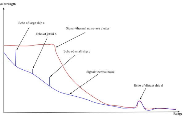
One of the problems that led to this work is that, depending on the state of the sea, there can be sea clutter (aka marine noise) which comes from the sea waves that backscatter the electromagnetic signal (aka the pulse of the radar) quite significantly, generating radar echoes of power comparable to the useful echoes coming from the marine targets. Fig. 1.1 illustrates the problem of the sea clutter: it is clear that the sea clutter can be problematic by hiding targets: targets a, b and c are undetectable because of the sea clutter. In addition to this sea clutter, there is the thermal noise from the radar device itself. It is important to note here that a radar signal will always contain thermal noise from itself. However there will not always be sea clutter, which depends on the sea state (i.e., a very calm sea does not result in a signal containing sea clutter).

To mitigate the problem of lack of real radar data, researchers tend to simulate new data by studying the ability to represent the backscatter from the sea in statistical terms using various statistical models. The simulator produces radar images imitating images taken with a rotating non-Doppler radar on board an aircraft and moving at a variable altitude. Eq. 1.1 shows how the simulated image is created by adding the target signal to thermal noise and sea clutter.

(19)

Signal strength

Range

Signal+thermal noise+sea clutter Echo of large ship a

Echo of jetski b

Echo of small ship c

Echo of distant ship d Signal+thermal noise

Figure 1.1: The sea clutter problem, the receiver is saturated by the clutter, making the ship a, b and c undetectable with sea clutter but detectable without it. In red: the signal+thermal noise+sea clutter. In blue: the signal+thermal noise.

Radarimage = Target + Noisethermal+ Noisesea-clutter (1.1)

Noise in radar signals is a significant problem in marine detection and sea clutter is the most problematic. Instead of developing an End2End system doing the detection, we propose to first conduct a denoising of the data and then train a model to carry out the detection on the denoised data. Sec. 1.1 will state the main question of this chapter, while the actual situation with radar signal denoising will be presented in sec. 1.2. Sec. 1.4 will show the proposed approach for denoising in radar signals. The experimentation for denoising in radar signals will be featured in sec. 1.5, including: denoising for better segmentation, unpaired denoising and the proposal of denoising with real data. Sec. 1.6 will present why using deep learning for denoising is a good idea and sec. 1.7 will show why it works better with a pre-denoising. Finally, sec. 1.8, conclude this chapter.

1.1 Main question

The question we want to answer in this chapter: How can we conduct a pre-processing denoising in order to increase the performance of a system for a subsequent task ?

To simplify the problem, experimentation will be conducted with a single model in a specific frame using synthetic images. The synthetic images are from a radar simulator. Two types of noise will be

(20)

present in these images, a conventional noise (Gaussian type, thermal noise) and a more random noise with structures according to a K law (sea clutter). The positive answer to this question will allow us to give a functional technique that supports the main hypothesis made in this thesis, which is that it is possible to include information in training that is not available in testing to augment the performance of a system.

1.2 Actual situation with radar signal denoising

Traditionally, in the field of radar detection, minimal or no denoising pre-processing is carried out on the signal. When denoising techniques are used, they usually precedes the technique for detection in radar signals and are either basic methods (e.g. sliding sum of samples to smooth the noise) or conventional signal processing methods such as local transform-based denoising [12], wavelet-Based denoising [13] and binary integration denoising [14]. The recent literature has shown that these denoising techniques are suboptimal compared to state of the art deep learning based denoising methods [15; 16], a comparison with conventional denoising techniques will be made in sec. 1.6.

1.3 Metrics for the subsequent task

Several metrics are used to quantify the performance of a detection system, the task conducted after the denoising proposed here. The three metrics for pixel detection are interrelated: sensitivity, specificity and accuracy. They are some of the most widely used metrics in signal processing.

The sensitivity, or True Positive Rate (TPR), defined as :

TPR = TP/P = TP/(TP + FN), (1.2)

measures the proportion of actual positives that are correctly identified as positive. True Positives (TP) is the number of detections that actually correspond to a vessel, False Positives (FP) is the number of false detections, True Negatives (TN) is the number of times when nothing was detected while there was nothing to detect and False Negatives (FN) is the number of missed detections.

Specificity,or True Negative Rate (TNR), computed as:

TNR = TN/N = TN/(TN + FP) (1.3)

measures the proportion of actual negatives that are correctly identified as negative. Finally the accuracy obtained by:

(21)

High Sensitivity

Few False Negatives (blue)

Low Specificity

Many False Positives (red)

Low Sensitivity

Many False Negatives (blue)

High Specificity

Few False Positives (red)

Mark as negative Mark as positive Mark as negative Mark as positive

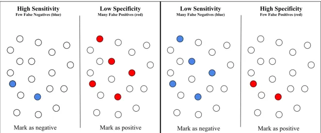
Figure 1.2: Illustration of sensitivity and specificity. The left part is a first experiment and the right part a second experiment.

Fig. 1.2 shows the general example of high sensitivity and low specificity on the left, and of low sensitivity and high specificity on the right. The pixel metrics to look at in order to make the most enlightened decision easily is the sensitivity, because accuracy and specificity have T N in their formula, which in our case can be biased by the fact that there is much more background than vessel in the target image.

Another relevant metric is a coverage metric called the dice coefficient. Eq. 1.5 is the one for the dice coefficient:

DSC = 2|X ∩ Y |/(|X| + |Y |) (1.5)

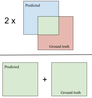
The dice coefficient measures the similarity between set X and set Y , in this case set X is the output of a predictor, while set Y is the ground truth. Given a model that outputs a 2D map of the location of the vessels, set X and Y are the pixels that indicate the positions of these vessels in the network output and its corresponding ground truth. If the two sets are identical, the dice coefficient is equal to 1, if they have no element in common, the value is 0 and otherwise it is somewhere between the two values. Fig. 1.3 show the calculation of the dice coefficient with an illustration. Among all the metrics presented, it is this one that gives the best idea of segmentation performance (segmentation of vessels), a task containing detection.

The detection accuracy is also a very important metric. We defined a target as detected if it is associated with one true detection at least. A pixel is considered a true detection if it is classified as a positive and lies in the neighbourhood of a target in the ground truth. This neighbourhood is defined with a localization error margin on both range and bearing axis, such as 50 m for the range error margin and 0.5 degrees for the bearing error margin. To convert these values in terms of pixel neighbourhood, it is necessary to divide them respectively by the range sampling and bearing sampling metadata values. A true detection is always associated to a specific target, and can thus refer to his target ID. In other

(22)

+

Predicted Ground truth Predicted Ground truth

2 x

Figure 1.3: Illustration of the calculation of the dice coefficient, the green parts are used in the calculation.

words, a detection of a target is said to be confirmed when a detection pixel falls within the target region, and only one pixel is required.

The search for a new metric A very important characteristic that these various metrics (accuracy, sensitivity, specificity, dice coefficient and detection accuracy) do not allow is the direct measurement of the number of false detections not related to a detection: a blob (i.e., a blob is simply a cluster of contiguous pixels) of detected pixels (white) which is really not in the neighbourhood of a target in the ground truth. The probability of detection is defined as the total number of targets detected divided by the total number of targets in the ground truth. A detection is if a detection pixel has fallen into the target region (i.e., one target pixel is detected at least). Measures that provide an idea of the number of false detections not related to a detection are the false alarm rate (FAR = FP/(FP + TN)), but this metric is pixel related not blobs related and again contains TN, and the dice-coefficient, which is a segmentation metric and not a detection metric. In the current case a good segmentation mask is less important than good detections. It should be borne in mind that ultimately an airplane pilot will have to look at the image and determine if a detection on his radar screen is a vessel or not and thus ensure the safety of a possible mission.

The new metric proposed must be able to take into consideration the number of good blobs (true positive blobs) in the image on the number of targets, but also the number of bad detections, blobs that can be considered as a target, but not being one (False positive blob). We will finally use two additional metrics to quantify the detection in blob format. The first measure is the Blobaccuracy, which

(23)

Blobaccuracy =

TPB

TPB + FNB (1.6)

where TPB is the number of true positive blobs while FNB is the number of false positive blobs. The second measure is the Network Dropout, which is calculated as follows

Blobrecall=

TPB

GTB (1.7)

where TPB is the number of true positive blobs while GTB is the number of blobs in the ground truth segmentation mask.

We already have access to the total number of targets and the number of detections made by either the model. The only missing information is the number of blobs in each radar acquisition qualifying as detection. For the following, the algorithm used is the SimpleBlobDetector from OpenCV, it used the connected-component labeling algorithm [17], which allows a perfect blob detection to be obtained and several parameters to be adjusted to filter the obtained blobs. The crucial parameter to filter the obtained blob is the minimum area for a blob to be considered as a potential detection. To decide on the value of this parameter, it was necessary to vary it and observe the resulting blobs. The objective was to look for the smallest blobs that a network generates and that count for a true detection. An area of about 50 pixels was then found (an image is 512x512 pixels). To summarize, the objective with an area of 50 pixels is to look for the smallest blob that counts as a true detection, but also all the other blobs larger than this size that do not necessarily count as a true detection and that are ignored by the detection accuracy metric. The only disadvantage of these two metrics is that they are relatively long to obtain, because after passing the blob detector on the prediction, a human has to compare these images to the real segmentation masks to determine the number of good and bad blob in the prediction. It was decided not to automate this task, as the objective here is to see the effect on detection by humans. It is a human who has to decide whether it is a target or not in the end. An arbitrary percentage of common pixels to qualify a good detection is not a good measure here, because sometimes it is very clear that a vessel in this area is a vessel even if the mask is relatively different from the GT. The two metrics (Blobaccuracyand Network Dropout) will not be calculated for each of the 5 models of each experiment.

They will be calculated only for the model closest to the average.

We decided to prepare a better illustration of the Network Dropout vs. Blobaccuracytrade-off, providing a

top view (the z-axis, being the profits coming out of the screen) illustrating the method maximizing profit (i.e. in economic terms, a gain is a money input and a cost is a money output, Profit = Gain − Cost), which is calculated in the following way:

Profit = Gaingood blob∗ Blobrecall− Costbad blob∗ (1 − Blobaccuracy) (1.8)

Fig. 1.4 is an example the recall vs. accuracy compromise which indicates that the best model would be model 1, which has the largest area. In the next section, the technique to do the denoising preceding

(24)

0 200 400 600 800 1000 Cost bad blob (1-accuracy)

0 200 400 600 800 1000

Gain good blob (recall)

Model 1 Model 2

Figure 1.4: Recall vs accuracy compromise, example. Model 1 have a Blobrecallof 0.8 and a Blobaccuracyof 0.9, while model 2 have a Blobrecallof 0.7 and a Blobaccuracyof 0.95.

the segmentation/detection task will be explained.

1.4 Proposed approach for denoising

The proposed approach for denoising will be based on deep learning. It will use the generative adversarial method using an encoder-decoder architecture as backbone for data-driven denoising. But first of all an experiment will be done to see if denoising can really increase segmentation performance.

1.4.1 Statistical test

Here we will present the statistical test that will be used throughout this thesis. The test used is the well-known Wilcoxon-Mann-Whitney (WMW) test to determine if two sample populations are significantly different or are from the same distribution [18]. We use the non-paired version based on the rank-biserial correlation [19]. The null hypothesis here is that two samples are from the same distribution while the alternative hypothesis is that they are not from the same distribution. The null hypothesis is rejected if the pvalueobtained by the WMW test is smaller than the α value set at that time

(normally between 0.1 and 0.01).

1.4.2 Baseline for detection in radar signals

The baseline used here is an End2End segmentation network whose details will not be disclosed for confidentiality reasons, we can on the other hand reveal that it is a kind of convolutional neural network

(25)

Accuracy Sensitivity Specificity D-C

All noises 0.993 0.885 0.996 0.833

Thermal noise 0.993 0.975 0.994 0.843

Table 1.1: Thermal only vs all noises. Statistically significant results are in bold, WMW test with an α of 0.01. Type of boat All noises Thermal noise

Jetski 65.7% 92.9%

Fishing boat 95.7% 98%

Frigate 100% 100%

Cargo 100% 100%

All 82.4% 95.8%

Table 1.2: Results of all noises vs thermal noise for detection accuracy. Statistically significant results are in bold, WMW test with an α of 0.01.

that takes X as input and predict Y . In this chapter when we refer to a segmentation network it is this baseline we are referring to.

1.4.3 Segmentation without sea clutter

In this subsection, we are looking to see if performance is better on data that simply contains thermal noise in comparison with data containing sea clutter in addition.

Two baseline segmentation networks were trained (each five times) on the same training set and tested on the same test set. However, in one case the images had only thermal noise, while in the other cases both types of noise were present. Details of the training methodology are confidential.

The results in tab. 1.1 show that images containing only thermal noise give better performance in segmentation/detection than the segmentation network with all the noise. The dice-coefficient has been improved by 1.2%, but the sensitivity has been improved by 10.2%, while tab. 1.2 shows a gain of more than 13% in detection accuracy by using thermal noise only. With the data we have at our disposal and the problem we are trying to solve, it is possible to conclude that a denoising of data (i.e., from sea clutter + thermal noise to thermal noise only) could be beneficial for segmentation/detection performances; the next section will look at this.

1.4.4 Generative adversarial network

Generative adversarial network (GAN) will be used throughout this thesis, and it is therefore necessary to present this technique in detail. GAN has been proposed by Goodfellow [20] in 2014.

In style transfer, GANs are state of the art [21]. In [22] the authors investigate conditional adversarial networks as a general-purpose solution to Image-to-Image translation problems and proves its usefulness and superiority in many different applications. In [23], the authors extend the idea of the

(26)

Image-to-Training data c x Discriminator D(c,x) Generator G(c,z) z x̂=G(c,z) L1 loss Fake pairs Real/fake pair? (GAN loss) Real pairs

Figure 1.5: Image-to-Image translation with conditional adversarial networks.

Image translation to a case where this time there is no need to have pairs of images. In this work it is the first of these two techniques that is used and therefore presented in detail here. Fig. 1.5 illustrates the training strategy of a conditional generative adversarial network (CGAN) for Image-to-Image translation. To summarize, the network takes an image c as input; the generator then transforms this image into a false image x; a discriminator takes two pairs from it: one formed of this false image x and the image c and one formed of the true image x (i.e., the ground truth) and the image c and must say which pair is true and which pair is false. With these results a loss is calculated and the generator and discriminator are updated (i.e., a pixel-wise loss is always used in addition in those problems). Nowadays, this loss is very often combined with a perceptual loss [24; 25] to increase the accuracy of the transfer, but the basic principle remains exactly the same.

These techniques are now used in a wide variety of fields, from art to medicine: it is used transform a photo to a painting in the style of a specific painter (with the unpaired version [23]) and also in medicine to help diagnose disease with segmentation and denoising [26]. But denoising with CGAN is also popular outside the medical spectrum. Indeed it is very useful in image reconstruction including deraining [27], desnowing [28] and dehazing [29], which will be covered in Chapter 2.

1.4.5 Denoising model

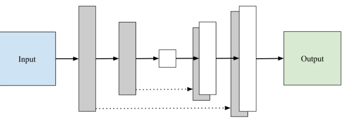
The denoising model involves an adversarial type of training with a CGAN. The generator uses the same network as in [22] (i.e. a U-NET [30]) and the same discriminator (i.e., a PatchGAN discriminator [22]) is also used. As shown in fig. 1.6, the U-NET consists of two main parts: the first one being the encoder, which is simply a stack of convolution layers with max pooling layers that captures the context of the

(27)

Input Output

Figure 1.6: U-net architecture (example with a depth of 3). The arrows denote the different operations. The dotted arrow represents the skip connection.

more recent article; that bilinear upsampling gives similar results as transposed convolutions with less parameters [27; 31].

The loss function of the generator is as follows:

Lgenerator= LGAN+ λ1Lpixel (1.9)

where LGANand Lpixelare themselves loss functions on specific elements of the task and λ1is weighting

relative influence in a linear combination; λ1is set to 10 here, and this value of λ comes from [22]

LGANis the loss function from Isola et al. [22] used to generate fake images:

LGAN = Ex,y[logD(x, y)] + Ex,z[log(1 − D(x, G(x, z)))] (1.10)

Lpixelis the reconstruction loss between the real non-sea-clutter image and the fake non-sea-clutter

image, based on their individual pixel values, allowing the network to produce crisper images:

Lpixel= Ex,y,z[ky − G(x, z)k1] (1.11)

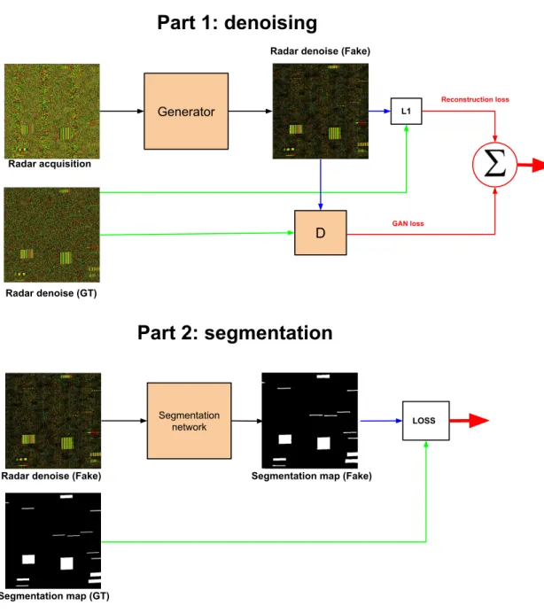
The objective of the generator is to generate an image with only thermal noise as close as possible to the ground truth without sea clutter, whereas the objective of the discriminator is to accurately indicate whether an image comes from the generator or is a real image. The generator tries to beat the discriminator and vice versa. Denoising with only the U-NET was also tested. However, according to preliminary tests on a validation set, the denoising was better using a GAN. After having trained the denoising network, we propose to use the latter when training a new segmentation network, so the network will have to start from the false image without sea clutter and go to the segmentation mask. Fig. 1.7 shows the proposed system.

(28)

Part 1: denoising

Generator L1

Radar acquisition

Radar denoise (Fake)

Radar denoise (GT) D Reconstruction loss GAN loss Segmentation network LOSS

Radar denoise (Fake)

Segmentation map (GT)

Segmentation map (Fake)

Part 2: segmentation

Figure 1.7: Proposed denoising+segmentation/detection model scheme. For the first part, the U-NET 1 is the generator of the denoising system while the D is the Patch-GAN discriminator. For the second part, the network used is the baseline segmentation network.

(29)

1.5 Experimentation and results for denoising

In the following we are investigating if it is possible to use the fact that we have access to data containing different noises in addition to the segmentation masks during training. Even if as test time we assume that we only have access to one type of data (i.e., the signal captured by the radar).

1.5.1 Denoising for better segmentation

Previously we demonstrated that performance is better on data that simply contains thermal noise. In this subsection we want to verify if it is possible to remove sea clutter in order to increase the system’s performance with a training using paired data.

To do the denoising a training set containing 5000 pairs of images is used, and the validation set is composed of 10% of the training set. The network is trained using a batch size of 16, each model is trained 5 times for 100 epochs (i.e., until convergence is reached on the validation set), the reported performance is the average and the WMW test is used to establish the statistical significance of the tests. Fig. 1.8 qualitatively shows how the denoising can remove sea clutter.

Later this network was tested on noisy inputs from a test set (containing 200 images) to see how it improved the performance in segmentation of a network trained on inputs with thermal noise only, but the results were not conclusive. However, a problem is that these denoised data may be quite different from those with thermal noise only used to train the network called S-T. There is absolutely no guarantee that the denoised data are of the same distribution as the thermal noise only data. A simple visual check leads to the conclusion that there are significant differences between the two types of data, see fig. 1.8.

To solve this problem, a segmentation network trained for the segmentation of denoised images was considered (i.e., this network is called S-T*, because it is an image with false thermal noise). This network is trained on 250 images having been previously denoised by the denoising network; the methodology of this training is kept confidential.

By comparing the results in tab. 1.3, it turns out that the S-T* system is significantly better than the S-T system in the present context. Tab. 1.4 presents the results of the model using deep learning with 250 images and 2500 images with and without denoising (aka the End2End model), while tab. 1.5 shows the detection accuracy using the deep learning (DL) model with 250 images and 2500 images with and without denoising. We can wonder if denoising suppressed small targets. According to tab. 1.5 the detection of small targets (e.g. jetski) is better for 250 and 2500 images with denoising.

It remains to be verified if denoising really leads to an improvement in the system’s performance according to Blobaccuracy and Blobrecall, the two metrics closest to the reality of detection in radar

(30)

Noisy input Denoise output GT denoise GT mask

Figure 1.8: Samples for denoising, from left to right: noisy input (thermal noise + sea clutter + targets), denoised output (false thermal noise + targets), GT (i.e., thermal noise image + targets) and finally the segmentation mask with targets in yellow and the background in purple.

S-T S-T*

Accuracy ↑ 0.989 0.994

Sensitivity ↑ 0.51 0.944

Specificity ↑ 0.999 0.995

Dice-Coefficient ↑ 0.616 0.856

Table 1.3: Results for denoising tests with 250 images, average of 5 different training. S-T is the segmentation network trained on the real images with thermal noise and applied in testing on the output of the denoising network, whereas S-T * is the segmentation network trained on the outputs of the images of the denoising network (i.e., false image with thermal noise) and applied in testing on the output of the denoising network. Statistically significant results are in bold, WMW test with an α of 0.01.

250 images 2500 images

End2End w denoising End2End w denoising

Sensitivity ↑ 0.885 0.944 0.96 0.97

Dice-Coefficient ↑ 0.833 0.856 0.87 0.875

Table 1.4: Results of the model using deep learning with 250 images and 2500 images with and without denoising. Statistically significant results are in bold, WMW test with an α of 0.01.

(31)

250 images 2500 images Type of boat w/o denoising w denoising w/o denoising w denoising

Jetski 65.7% 83.3% 81.6% 86.2%

Fishing boat 95.7% 95% 96.6% 95.7%

Frigate 100% 100% 100% 100%

Cargo 100% 100% 100% 100%

All 82.4% 90.0% 90.1% 91.7%

Table 1.5: Detection accuracy using the DL model with 250 images and 2500 images with and without denoising. Statistically significant results are in bold, WMW test with an α of 0.01.

250 images 2500 images

w/o denoising w denoising w/o denoising w denoising Blobaccuracy 95.6% 92.3% 86.7% 95.7%

Blobrecall 77.3% 87.0% 89.4% 89.6%

Table 1.6: Results of the model using deep learning with 250 images and 2500 images with and without denoising, according to a threshold of 50, higher is better. Using the model closest to the average according to testing performance (i.e., detection accuracy and dice coefficient) for each method. Results in bold are the best.

0 200 400 600 800 1000

Cost bad blob (1-accuracy) 0 200 400 600 800 1000

w/ Denoising w/o Denoising

Figure 1.9: Recall vs accuracy compromise for 250 images; with 2500 it is always better with denoising.

greatly increases the Blobrecall(an absolute gain of 10% for 250 images and 2500 images), therefore

more good blobs are detected. But still, the Blobaccuracy is better without denoising for 250 images.

We must be careful here, since this decrease of Blobaccuracy is explained by the fact that the network

without denoising simply did not lead to blobs in many potential locations (hence its Blobrecallis quite

low), while the model with denoising can detect nearly 90% of the blobs while keeping a satisfactory Blobaccuracy of nearly 90%. Fig. 1.9 presents the recall vs. accuracy trade-off for training with 250

images. In the vast majority of scenarios the best system is indeed the one using denoising.

A last experiment was conducted to check if a denoising of all the noises towards only the signal of the targets (i.e., then almost the mask of segmentation) would be beneficial for the performance in segmentation/detection. Again the segmentation was tested in two ways: either with a network

(32)

S-TS S-TS*

Accuracy ↑ 0.99 0.99

Table 1.7: Results for the denoise-target tests, average of 5 different training. S-TS is the segmentation network trained on the real images with target signals and applied in testing on the output of the denoise-target network, while S-TS* is the segmentation network trained on the outputs of the images of the denoise-target network (i.e., false image with signal of targets) and applied in testing on the output of the denoise-target network. Statistically significant results are in bold, WMW test with an α of 0.01.

trained on the real images of the target signal (called S-T for segmentation target signal) and the other network on the outputs of the denoising network (i.e., the false images of the target signal, called S-TS*). According to the results in the tab. 1.7, with the data at our disposal and the problem we are trying to solve, the denoising of all the noises towards the signal of the targets only does not offer better performances in segmentation than the End2End network and thus than the technique of denoising towards only thermal noise.

With the data we have at our disposal and the problem we are trying to solve it is possible to conclude that denoising all noises towards thermal noise only, followed by segmentation with the S-T* network provides better segmentation/detection performances than the End2End network.

1.5.2 Unpaired denoising

In the following, we are investigating the usefulness of unpaired training with a CycleGAN [23] for denoising to augment the performance in segmentation/detection in comparison to an End2End system. This will allow us to know if such an unpaired system should be used on real unpaired data (i.e., paired data: the image and the mask are from the same scene, the denoising with the CGAN is a paired training, where as in unpaired data: the image and the mask are not from the same scene).

For this experiment the same CycleGAN architecture proposed by Zhu et al. [23] is used. However three different loss functions will be tested. The first is the loss function taken directly from [23], this function is not possibly the best in this case, because it has a part called cycle-consistency loss, which means that we want to start from an image with noise, remove the noise and put exactly the same noise back into it. Such a manoeuvre is impossible for the sea clutter because its structure is random and does not depend on the image, but on the sea conditions. Fig.1.10 presents the structure of the classic CycleGAN.

The loss function of this CycleGAN is the following:

(33)

X Y Dx G F Dy x Ŷ x̂ Dy X Y cycle-consistency loss F G y X̂ ŷ Dx X Y cycle-consistency loss G F a) b) c)

Figure 1.10: (a) The model contains two mapping functions G : X→ Y and F : Y → X, and associated adversarial discriminators DYand DX. DY encourages G to translate X into outputs indistinguishable from domain Y , and vice versa for DXand F. To further regularize the mappings, we introduce two cycle consistency losses that capture the intuition that if we translate from one domain to the other and back again we should arrive at where we started: (b) forward cycle-consistency loss: x→ G(x) → F(G(x)) ≈ x, and (c) backward cycle-consistency loss: y → F(y) → G(F(y)) ≈ y

where LGANis the loss function used to generate fake images, for the mapping function G : X→ Y:

LGAN(G, DY, X, Y ) = Ey∼pdata(y)[logDY(y)] + Ex∼pdata(x)[log(1 − DY(G(x)))], (1.13)

the same logic is used for the mapping F : Y→ X, and where Lcyc is the cycle consistency loss:

Lcyc(G, F ) = Ex∼pdata(x)[||F (G(X)) − x||1] + Ey∼pdata(y)[||F (y) − y||1]. (1.14)

The second loss function (i.e., the GAN using it is called CycleGAN V1) used is the same as the previous one, but in this case we remove the cycle-consistency loss for the noise-denoise-noise side, but we keep the consistency loss cycle for denoise-noise-denoise, because this side makes more sense. The third loss function (i.e., the GAN using it is called CycleGAN V2) used is the same as the previous one, but in this case the consistency loss cycle for the denoise side is replaced by a noise-denoise-noise-denoise one (i.e., we then compare the two denoise), but we keep the same consistency loss cycle for denoise-noise-denoise. To carry out this experiment, it is necessary to use a batch size of 1 and also to resize the images to 256x256 (i.e., from 512x512) to allow loading on an 11GB graphics card. 5000 pairs of data are used for the training and, of course, each pair is random in this case (i.e., a pair has an image with and without noise, but they are not the same image, they are unpaired). Studies have also shown that a batch size of 1 is often the optimal for a CycleGAN [23].

Fig. 1.11 presents the results of the denoising; at first it seems that the three models output exactly the same image. At this point one may wonder if it was not the same model. However, by making the difference between the images, we obtain a mask that contains variations of intensity (i.e., differences), see fig. 1.12 . So it is possible to conclude that even with the modification of the GAN loss function it

(34)

Input Ground truth CycleGAN CycleGAN V1 CycleGAN V2 Figure 1.11: Qualitative examples for denoising radar images using CycleGAN. From left to right: noisy input, ground truth output using normal CycleGAN, output using CycleGAN V1, output using CycleGAN V2.

seems that the three versions converge towards the same region in the parameter space. The images in fig. 1.11 also indicate that denoising is not satisfactory with the CycleGAN. Indeed, it seems that the distribution without sea clutter is approached according to colour, but the structures of the sea clutter are still present, while the paired denoising introduced earlier allowed the removal of most of these structures to reveal hidden targets (see fig. 1.8). Tab. 1.8 presents the quantitative results, which clearly indicate that, with the data at our disposal and the problem we are trying to solve, pre-denoising with CycleGAN does not help the system’s performance and is rather detrimental compared to simply using an End2End system.

What explains these poor performances? There is a significant potential problem with the data. Images with thermal noise plus sea clutter sometimes contain only thermal noise. Indeed sometimes since the sea is very calm, the image does not contain sea clutter, even if it is tagged as an image containing all the noise including sea clutter. To conduct a suitable training with a CycleGAN it is necessary to have images with the right tag, while in paired training (i.e., Pix2Pix) the network must switch from an image with marine plus thermal noise to only thermal noise, so the network can easily understand that sometimes it is given an image with only thermal noise as input and then the output is the same as the input. However, the CycleGAN must also start from an image with thermal noise and add sea clutter.

(35)

CycleGAN CycleGAN V1 CycleGAN V2 Diff(1-2) Diff(1-3) Figure 1.12: Qualitative examples for denoising radar images using CycleGAN. From left to right: output of CylceGAN, output of CycleGAN V1, Output of CycleGAN V2, absolute difference between the 1st and 2nd column, absolute difference between the 1st and 3rd column. The difference is shown using a colour map ranging from blue (low) to yellow (high), highlighting regions in the image where the most difference is present.

CycleGAN End2End

Accuracy ↑ 0.973 0.99

Table 1.8: Results for tests of CycleGAN denoising for segmentation, average of 5 different trainings. For the CycleGAN, the segmentation network is trained on the outputs of the images of the denoising network (i.e., false image with thermal noise) and applied in testing on the output of the denoising network. Reminder: both networks are trained with 256x256 images instead of 512x512. Statistically significant results are in bold, WMW test with an α of 0.01.

This should be fine, except that there are data tagged as sea clutter without any sea clutter. The whole system is interlinked and thus, if one part is deficient, the whole system will be.

Even if the performance is worse with an unpaired CycleGAN than without, this denoising remains relevant and has raised a good question. Why, fundamentally, should we use an unpaired CycleGAN training rather than a paired Pix2Pix training? To answer this question properly, we must go back to the origin of the CycleGAN, which was created to solve a very specific problem at the beginning. It is impossible with a Pix2Pix training to put a painter’s style into a photograph (i.e., transform a photo

(36)

into a painting), because this photo does not yet exist in the form of a painting with the painter’s style. This is where the CycleGAN enters the arena. By introducing an unpaired-style training, it is now possible to learn the painter’s style and apply it to photos without first requiring the ground truth of this photo in the form of a painting. So the CycleGAN is very useful for transferring from one style to another, but when it is possible to have paired data, its complexity is not worth it. In this case, with radar image denoising, the goal is to shift from an image with marine plus thermal noise to an image with thermal noise only. It is true that for real data, an unpaired CycleGAN training seems logical a priori. Nevertheless in the present context it would be possible to make paired datasets allowing paired denoising. However the details will not be disclosed for confidentiality reasons.

1.6 Why use deep learning for denoising?

To demonstrate the usefulness of deep learning for this denoising, it is necessary to compare with more conventional denoising methods (i.e., signal processing method). Here different classic denoising techniques are tested, including wavelet and total variation. Random searches were conducted to determine the optimal parameters for each method using a validation set, which was composed of input images (i.e., with all of the noise) and of target images (i.e., without any noise, including thermal noise, just the raw signal of targets). To measure the similarity between a denoised image and a target image we used PSNR (i.e., all validation decisions are made using the PSNR). Here the target is only the target signal, so no noise. In fact it is not possible to request that the conventional method to only remove the noise of the sea clutter; these techniques will try to remove all of the noise in the image. The first denoising technique used is wavelet denoising, a strong and popular conventional denoising technique. The simple idea at the basis of wavelet denoising is that the transformation into wavelets leads to a scattered representation for many real world signals. This implies that the wavelet transforms concentrate the signal characteristics into a few large amplitude wavelet coefficients. The low value wavelet coefficients are usually noise and you can reduce or remove them without affecting the quality of the signal. Once a threshold is set for the coefficients, the data is reconstructed using the inverse wavelet transform. For the thresholding approaches of the wavelet coefficient there are two principal options: BayesShrink, an adaptive thresholding method that computes separate thresholds for each wavelet sub-band [32] and VisuShrink, a universal threshold is applied to all wavelet detail coefficients [33]. For both wavelet-based denoising methods (i.e., BayesShrink and VisuShrink), different wavelet shapes were tested and the best one in both cases was the classic Daubechies 1 (db1). A third approach using wavelet BayesShrink denoising and tested here is Cycle Spinning which was created to approach shift-invariance via performing several cycle shifts of a shift-variant transformation [32].

The second denoising technique used is total-variation denoising (TV) which attempted to find an image with the least total variation possible under the constraint that the denoised image must be similar to the noisy image which is controlled by the weight parameter. So more denoising gives less similarity with

(37)

Input DL Wavelet BayesShrink Wavelet VisuShrink GT Mask Figure 1.13: Samples for denoising with conventional method, from left to right: noisy input (thermal noise + sea clutter + targets), DL denoising, Wavelet BayesShrink denoising, Wavelet VisuShrink denoising and finally the segmentation mask with targets in white and the background in black.

the noisy image. Two methods for total variation denoising were tested, one using the split-Bregman optimization [34] and the other using the Chambolle optimization [35]. For both methods a random search between 0.001 and 100 was made to determine the value of the weight parameter, which was 0.05 for split-Bregman and 20 for Chambolle.

The same methodology as with denoising using deep learning is used here. In fact the conventional denoising algorithm is applied on the training data (250) and then we trained the segmentation network on the denoised images. This is again the same system in two steps, the only difference being the technique to obtain the images without sea clutter for deep learning and without any noise for conventional denoising. The methodology to train the segmentation model is also exactly the same as before and still confidential.

Tab. 1.9 shows the results in segmentation according to the dice coefficient for the different conventional denoising techniques and for the technique using deep learning. According to these results, the two best techniques are wavelet BayesShrink and DL. However the difference is not significant according to the WMW test. Tab. 1.10 gives a better idea, with the detection accuracy, of the real winner between these two methods. Indeed the denoising technique using deep learning is far superior to wavelet

(38)

Wavelet B TV Ch CG TV Br Wavelet V DL

Dice coefficient ↑ 0.857 0.16 0.835 0.615 0.828 0.856

Table 1.9: Results for conventional denoising for sensitivity and D-C, here DL is with denoising. Wavelet B if for Wavelet BayesShrink, TV Ch refers to TV Chambolle, CG refers to Cycle spinning, TV Br refers to TV Bregman, Wavelet V refers to Wavelet VisuShrink and DL refers to deep learning.

Type of boat Wavelet B TV Ch CG TV Br Wavelet V DL

Jetski 66.5% 29.6% 62.3% 33.0% 57.3% 83.3%

Fishing boat 95.2% 54.9% 94.7% 82.5% 93.2% 95%

Frigate 100% 67% 98.4% 98.4% 100% 100%

Cargo 100% 100% 100% 100% 100% 100%

All 82.6% 45.5% 80.4% 61.3% 77.2% 90.0%

Table 1.10: Results for conventional denoising for detection accuracy, here DL is with denoising. Wavelet B if for Wavalet BayesShrink, TV Ch refers to TV Chambolle, CG refers to Cycle spinning, TV Br refers to TV Bregman, Wavelet V refers to Wavelet VisuShrink and Dl refers to deep learning. Statistically significant results are in bold, WMW test with an α of 0.01.

Wavelet B DL 250

Blobaccuracy 97% 95.8%

Blobrecall 77% 87.7%

Table 1.11: Results of the segmentation network with 250 images with DL denoising and Wavelet B (Wavelet BayesShrink) denoising, according to a threshold of 50, higher is better. Using the model closest to the average according to testing performance (i.e., detection accuracy and dice coefficient) for each method. The best results are indicated in bold.

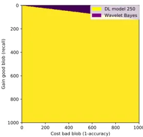
BayesShrink, the runner-up, the difference being significant this time according to the WMW test with an α of 0.01. Fig. 1.13 presents samples of denoising with DL, wavelet BayesShrink and wavelet VisuShrink. It appears that the best denoising method is DL. Wavelet VisuShrink seems too strong, some targets disappear completely, and wavelet BayesShrink generates strange structures (top row). Blobaccuracy and Blobrecallcan better compare DL and wavelet BayesShrink. According to tab. 1.11

the best method based on the Blobaccuracy is wavelet BayesShrink (although the difference with DL is

small), while the best technique based on the Blobrecallis clearly DL (this time the difference is much

larger). As shown in fig. 1.14, illustrating the Blobaccuracyvs Blobrecalltrade-off, the best technique is

undoubtedly the deep learning denoising.

But why does deep learning lead to a better denoising than conventional methods? One hypothesis is the following: if we consider the best conventional method, wavelet BayesShrink, the shape of the wavelet is decided in advance; it is a generic method. Denoising with deep learning is a data-driven method that allows to learn a specialized denoising method to be learned for a problem, in this case data including sea clutter. So the conventional denoising method is more generic, while the deep learning method is more specialized. Fig. 1.15 presents samples of denoising with DL and wavelet BayesShrink with the resulting segmentation mask. It seems that the wavelet BayesShrink denoising method has difficulty with areas with a lot of sea clutter, while DL denoising does a relatively good job.

(39)

0 200 400 600 800 1000 Cost bad blob (1-accuracy)

0 200 400 600 800 1000

DL model 250 Wavelet Bayes

Figure 1.14: Recall vs accuracy compromise for DL denoising and Wavelet BayesShrink for 250 images.

Input DL DL mask Wavelet B Wavelet B mask GT Mask

Figure 1.15: Samples for segmentation of denoising conventional vs deep learning methods, from left to right: noisy input (thermal noise + sea clutter + targets), DL denoising, DL denoising mask, Wavelet B (BayesShrink) denoising, Wavelet B (BayesShrink) denoising mask and finally the segmentation mask with targets in white and the background in black.

(40)

1.7 Why the approach works better with a pre-denoising ?

The hypothesis is the following: the use of pre-denoising leads to a network specialized in denoising and another one specialized in segmentation of denoised images. This makes it easier for the segmentation network to work on denoised images than on images with noise; it has a greater capacity to do the segmentation. Fig. 1.16 shows that it is much easier to locate targets in denoised images than in noisy images, so the work is easier for a segmentation network. Indeed, the End2End network has to complete both tasks with the same number of weights as the segmentation model alone. Starting from an image with noise the network segment the image, so implicitly the network conducts a denoising at the same time but with no access to the real signal without sea clutter to guide this denoising. So to answer the principal question of this chapter, with the data we have at our disposal and the problem we are trying to solve, it is possible to conclude that we can use the fact that we have access to data containing different noises in addition to the segmentation masks during training, even if in testing we assume that we only have access to one type of noisy data (i.e., the signal captured by the radar) using the proper technique.

Noisy input Denoised output GT Mask

Figure 1.16: Why pre-denoising improves the situation. From left to right, the noisy input, the output the denoising network and the ground truth segmentation mask.