Numerical Study of Bio Fuels Combustion

(1)

PEOPULE'S DEMOCRATIC REPUBLIC OF ALGERIA

Ministry of Higher Education and Scientific

Research

University of Echahid Hamma Lakhdar – El-Oued

Institute of Exact Sciences

A Dissertation Submitted to the Department of Physics

In Partial Fulfillment of the Requirements

For the Degree of Master in

Applied Physics: Radiation and Energy

by: Nadjet GHERAISSA

Title

Members of jury:

Dr. Samia DILMI MCB University of Echahid Hamma LakhdarEl-Oued President Dr. Fethi BOURAS MCA University of Echahid Hamma LakhdarEl-Oued Supervisor Dr. Fathi LETAIM MAA University of Echahid Hamma LakhdarEl-Oued Examiner

N° d’ordre : N° de série : N° d’ordre : N° de série :

N

u

m

e

r

i

c

a

l

S

t

u

d

y

o

f

B

i

o

F

u

e

l

s

C

o

m

b

u

s

t

i

o

n

(2)

First of all I would like to thank God, the almighty for providing me

this opportunity and granting me the capability to finishing this

master thesis.

I would like to convey my sincere gratitude to my thesis supervisor

D

r

.

F

e

t

h

i

B

O

U

R

A

S for the guidance, encouragement throughout the

S

development of this work.

I would especially like to thank the members of the reading

committee

D

r

.

S

a

m

i

a

D

I

L

M

I

&

D

r

.

F

a

t

h

i

L

E

T

A

I

M for their

M

acceptance to examine my thesis.

I also wish to thank

M

r

.

M

.

E

.

A

T

I

A & my uncle

A

S

l

i

m

a

n

e for

e

helping me.

I convey my sincere thanks to my friends:

R

a

b

a

b

,

F

a

t

i

m

a

,

A

m

e

l

,

L

a

i

l

a

.

Last but never least, I want to express my deep thanks to

my dear parents for encouragement and support

throughout my life.

N

(3)

T

o

M

My

y

F

Fa

at

th

he

er

r

&

M

My

y

M

Mo

ot

th

he

er

r

......

T

o

Al

A

ll

l

M

My

y

F

Fa

am

mi

il

ly

y

(4)

T

a

b

l

e

o

f

C

o

n

t

e

n

t

s

List of Figures I

Nomenclature III

General Introduction 9

CHAPTER I

Turbulent Non Premixed Combustion Modeling

I.1 Turbulent Flow 13

I.2 Statistical Description of Turbulent Flows 14

I.2.1 Reynolds Average 14 I.2.2 Compressible Navier-Stokes Equations 14 I.2.3 The Kolmogorov Theory 17

I.3 Turbulent Dynamics Model 19

I.3.1 Large Eddy Simulation 19 I.3.2 The Governing Equations of LES 20 I.3.3 Sub-grid Scale Models for LES 21 I.3.4 WALE Model 21

I.4 Probability Density Function Model for Combustion 23

I.4.1 Properties of PDF 23 I.4.2 The Beta-PDF Approach 25 I.4.3 Non-Premixed Combustion Modeling 26 I.4.4 Progress Variable 26 I.4.5 Mixture Fraction Equation 27

Conclusion 28

CHAPTER II

Numerical Study of Combustion by CFD

II.1 Computational Fluid Dynamics 30

II.2 Fluent CFD 31

II.2.1GAMBIT 31

II.2.2 FLUENT 31

(5)

II.3 Steps For CFD Analysis 31

II.3.1 Step 01: Creating And Meshing Basic Geometry 31 II.3.2 Step 02: Opening Fluent 32 II.3.3 Step 03: Grid 33 II.3.4 Step 04: Define Solver Properties 34 II.3.5 Step 05: Define Material Properties 35 II.3.5 .1 Mixture Materials 35 II.3.6 Step 06: Define Boundary Conditions 36 II.3.7 Step 07: Non Adiabatic PDF Table 37 II.3.8 Step 08: Solution 39 II.3.9 Step 09: Analyze Results 40 II.3.9.1 Display Contour & Vectors 40 II.3.9.2 Drawing The Graphs 42

Conclusion 43

CHAPTER III

Results & Discussion

III.1 Experimental Configuration and Application Domain 45

III.1.1 The Experimental Configuration 45 III.1.2 Governing Equations 46

III.2 Results and Discussion 47

III.2.1 Validation of Numerical Models 48 III.2.1.1 Axial Velocity of CH4/Air Combustion 48 III.2.1.2 Temperature of CH4/Air 50 III.2.1.3 Carbon Monoxide Mass Fraction of CH4 52 III.2.2 Comparison of Bio Fuel & CH4 54 III.2.2.1 Carbon Monoxide Mass Fraction 54 III.2.2.2 Temperature 56 III.2.2.3 Axial velocity 58

Conclusion 60

General Conclusion 62

(6)

L

i

s

t

o

f

F

i

g

u

r

e

s

Figure I.1 Schematic presentation of turbulent jet. 13 Figure I.2 Illustration of the parameters decomposition in turbulent flow. 14 Figure I.3 Representation of DNS, LES and RANS with Kolmogorov energy spectrum,

Energy E(k) related to a wave-number k.

18

Figure I.4 Histogram together with it' s limiting PDF. 23 Figure I.5 Schematics of the progress variable distribution in the combustion. 27 Figure I.6 Surface of stoichiometric mixture (Zst) for a turbulent jet diffusion flame. 28

Figure II.1 Flow chart general CFD methodology. 30 Figure II.2 Combustion chamber design by GAMBIT. 32 Figure II.3 Window starting FLUENT version. 32 Figure II.4 Grid display. 33 Figure II.5 Graphic Display of Grid. 34 Figure II.6 Energy Equation solution. 34 Figure II.7 Definition of Transport & Reaction model. 35 Figure II.8 Materials Window. 36 Figure II.9 Boundary conditions of wall temperature. 37 Figure II.10 The Species Panel. 37 Figure II.11 Mean temperature as function for average mixture fraction. 38 Figure II.12 Temperature solutions from the equilibrium chemistry library for the Bio fuel

combustion.

38

Figure II.13 Residual of the equations during the iterations. 39 Figure II.14 Display Contour. 40 Figure II.15 Total temperature contours of Biofuel/Air. 41 Figure II.16 CO Mass Fraction Contours of Biofuel/Air.. 41 Figure II.17 X Velocity Contours of Biofuel/Air. 42 Figure II.18 Solution XY Plot panel. 42 Figure II.19 Plot of Total Temperature. 43 Figure III.1 Schematic of the burner 45 Figure III.2 Velocity distribution in the burner of CH4/Air combustion. 48

(7)

Figures III.3 Radial profiles of average axial velocity.___ Simulation (LES/PDF), •Experiment 49 Figure III.4 Temperature distribution in the burner of CH4/Air combustion. 50 Figures III.5 Radial profiles of average temperature.___ Simulation (LES/PDF), • Experiment 51 Figure III.6 CO distribution in the burner of CH4/Air combustion. 52 Figures III.7 Radial profiles of average Carbon monoxide.___ Simulation (LES/PDF),

• Experiment

53

Figure III.8 CO distribution in the burner of Biofuel/Air combustion(3D). 54 Figures III.9 Comparison of CO mass fraction of CH4 and Bio fuel. 55

Figure III.10 Temperature distribution in the burner of Biofuel/Air combustion(3D). 56 Figures III.11 Comparison of Temperature of CH₄ and Bio fuel. 57 Figure III.12 Velocity distribution in the burner of Biofuel/Air combustion(3D). 58 Figures III.13 Comparison of X-Velocity in CH₄ and Bio fuel. 59

(8)

N

o

m

e

n

c

l

a

t

u

r

e

Latin letters:

A _{Deformation tensor} C Specific heat c Parameter progress Cs Smagorinsky coefficient Cw _{Constant WALE} D Diameter E Energy e Internal energy

F _{Field describes the rate of the conserved variables.} hi Enthalpy of species i

2

ij

g Velocity gradient resolved k kinetic energy

L Large-scale Kolmogorov flow N Number of chemical species

n Boundary-normal coordinate

ni The number of moles of the species i

p Pressure

P( ) Probability density function F( ) the probability function.

Pr Prandtl number

qR Radiative heat flux vector

Q _{Conserved variables.} R ideal gas constant Re Reynolds number

s Source Term

ij

(9)

t _Time

T Temperature u Velocity



u _{Velocity component}

Vi _{Mass diffusion velocity of species i}

xi The mole fraction of species i

y _{The distance to the normalized wall} yi Mass fraction of species i

Z Mixture fraction

Greek Symbol

:  _{Mass density}  Thermal conductivity  Thermal diffusivity  Stress tensor  Dynamic viscosity  kinematic viscosity µT Turbulent viscosity

 _{Small-scale Kolmogorov flow}

i

 _{Chemical production rate of species i}

ij

 _{Viscous stress tensor}

Γ( ) _{Gamma function}

ij

 Kronecker delta

Index:

f Chemical Species

i Components along the axes x, y and z

r Radial coordinate

(10)

Abbreviations

:

CFD Computational Fluid Dynamics CRZ _{Central Recirculation Zone} DNS _{Direct Numerical Simulation}

FPDF _{Filtered Probability Density Function} GUI _{graphical user interface}

LES _{Large eddy simulation}

PDF _{Probability Density Function} RANS Reynolds Averaged Navier Stokes

SGS _{Sub-grid scale}

(11)

G

(12)

he conversion of Biomass into useful energy is done through various types of processes. The choice of the type of conversion process depends on the type, quantity, raw material properties, but also by the end user, the latter being able to put constraints of cost, environmental, or related to a specific design project. Biomass has always been a reliable source of energy, from the first man-made fire up to the utilization of pelletized wood as a feed for thermal plants. Although the use of lignocellulosic feedstock as a solid Bio fuel is a well-known concept, conversion of mass into liquid fuel is a considerable challenge, and the more complex the Biomass gets (in terms of chemical composition) the more complicated and generally expensive the conversion process becomes [1]. The concurring phenomena of world energy need increasing and oil stocks decreasing have generated an increased interest toward Bio fuels in the last 10 to 20 years, although for most of the 20th century, research on Bio fuel closely depended on the price trend of petroleum. Bio fuels can be defined are fuels produced from biological material, a definition that can also be applied to renewable sources of carbon. Use of ethanol for lamp oil and cooking has been reported for decades (called spirit oil at the time) before Samuel Morey first tested it in an internal combustion engine in early 19th century. Ethanol then replaced whale oil before being replaced by petroleum distillate (starting with kerosene for lighting). By the end of the 19th century, ethanol was used in farm machinery and introduced in the automobile market. Oil-derived products replaced ethanol for most of the 20th century before being introduced again during the Arab oil embargo in the 1970s when the price of petroleum and its derivatives peaked [2].

Li Zhou et al (2015) are investigated in the experimental analysis of the excess molar enthalpy data of the ternary systems and the corresponding binary systems at T = 298.15 and 313.15 K at atmospheric pressure [3]. The experimental data are fitted using the Redlich–Kister rational polynomials. Where the binary systems mixtures are shown endothermic effect and strong asymmetric behavior at the measured temperatures [4]. In 2015, G. Gonca is studied the influences of steam injection on the adiabatic flame temperatures, and is verified the simulation code with experimental studies to determine and to compare the combustion characteristics of Bio fuels and conventional diesel fuel. The results show that that the alcohols combustion produce minimum NO emissions. And the injection of Bio fuels as a diesel engine fuel could be decrease pollutants [5]. Dimitrios et al (2014) are present experimental study to evaluate the effects of the blends of diesel fuel with different compositions in the combustion performance and exhaust emissions. Fuel injection and cylinder pressure diagrams. The results of

(13)

experimental heat release analysis of the acquired fuel injection pressure and the different physical and chemical properties of the Bio fuels flame behavior in the engine [6]. Cameretti et

al (2013) are discussed some aspects related to employment the liquid and gaseous Bio fuels in a

typical lean premixed combustor of a micro-gas turbine. In addition, the purpose checking is the effectiveness methods for supplying the micro-turbine with fuels from renewable sources. For the liquid fuel is modified position of the pilot injector to find the optimal combination of the injector location to minimizing the emissions in a wide range of the micro gas turbine operation supplied by both natural gas and gaseous Bio fuels[7]. Brynolf et al (2014) are compared the methane, Bio fuels, methanol and the natural gas as a fuels and their impact on the environment and their energy performance as raw materials. For this raison a transition to use of LNG (Life cycle assessment) is used to produce the methanol from natural gas to improve the overall environmental performance [8]. G.I. Pearman (2013) is examined the bio-physical limits of Bio fuels and bio-sequestration of carbon by solar radiation incident, and he is observed the efficiencies with which natural ecosystems and agricultural systems convert that energy to Biomass. The results demonstrate that the Bio fuels or bio-sequestration can only be a small part of an inclusive portfolio of actions towards a low carbon future and minimize the net emissions of carbon to the atmosphere [9]. Morales et al. (2014) are performed an optical and thermal analysis of the Bio fuel process using solar pyrolysis of orange peels. The solar radiation is applied as a unique source of energy using a parabolic-trough solar concentrator; and an optical analysis conduct to use a Monte Carlo ray-tracing method to provide the tridimensional description of the optical performance of the thermo-solar system. Also, the need to identify new renewable energy sources allows the demonstration the solid agro-industrial waste management approach. Where, the solar pyrolytic processes could become important methods for producing solar liquids fuels because of their potential for converting unlimited amounts of solar energy into chemical energy [10]. Han et al (2013) are studied the analysis of bio-based aviation fuels and compared it with petroleum fuel. A sensitivity analysis of the key parameters of fuel production is conducted to identify the most important factors impacting of the pollutants emission, showing the importance of Biomass fuels share in the overall efficiency [11]. Aguilar

et al (2013) illustrate a new experimental study based on the molar enthalpy analysis at

atmospheric pressure. Where this study is based on the ternary systems dibutyl ether (DBE) and butanol and 1-hexene at 298.15 K and 313.15 K. And, butanol and cyclohexane trimethylpentane (TMP) at 313.15 K. Whereof, the isothermal excess molar enthalpies is determined by using a quasi-isothermal flow calorimeter. The results show that the ternary systems show that the addition of the hexene decreases the endothermic effect of the ether-alkanol mixture [12]. Bouras

(14)

et al (2013) are investigated the entropy generation rate in the turbulent non-premixed

combustion of methane/air in the coaxial jets. Where, this work is based on the validation of this study with experimental referenced data .ie, of axial velocity, temperature and mass fraction of carbon monoxide (CO). The numerical calculations are carried out by FLUENT-CFD including an integrated entropy generation function in C++ language using UDMs. The results prove that the chemical reaction and the heat transfer entropy generation sources are more important responsible of thermodynamic irreversibilities while the viscous friction irreversibility is negligible [13].

This work addressed the numerical study of non-premixed combustion in a three-dimensional cylindrical chamber fueled by Biofuel/air. The present study focused on find thermo-chemical dynamic characteristics of the combustion reaction. Whereas, the system is handled by using the LES & PDF models. Where modeling and calculation are carried out by the software package FLUENT-CFD.

The parts of the thesis have been organized as below:

Chapter I:

Initially, we present mathematical models for each of the LES & PDF. And, how can be surmount the closure in the equations.

Chapter II:

After that, we give the most important stapes of modeling the non-premixed combustion in a three-dimensional cylindrical combustion chamber by FLUENT_CFD.

Chapter III:

Finally, a numerical results is verified by experimental data, and compared with the kinetic, thermal and chemical properties for specific locations in the combustion chamber.

(15)

C

H

_H

A

_A

P

_P

T

_T

E

_E

R

_R

I

_I

T

u

r

b

u

l

e

n

t

N

o

n

P

r

e

m

i

x

e

d

C

o

m

b

u

s

t

i

o

n

M

o

d

e

l

i

n

g

(16)

he turbulence has an effect which improve the reactive mixture. Whereof, the combustion modeling gives the opportunity in the combustion engines development. The progress in computational material and numerical process allows the accessibility to complex configurations. Nevertheless, the turbulent flow is characterized by the fluctuations; this makes the turbulent flows simulation very difficult. Thereby, the fluctuations are modeled by the method using statistical averaging calculations.

In this chapter, we are going to present a basic theory of turbulence based on the statistical analysis applying to the non-premixed combustion. Moreover, the two models are given in the next, and they are the key of interest of the prediction and the modeling flows: turbulence model of LES and the thermo-chemical model of PDF combustion.

I.1 Turbulent Flow

Turbulence is the chaotic state of fluid motion, which is characterized by apparently random and chaotic three-dimensional vorticity. When turbulence appears in the overall flow and dominate the phenomena including in the flows, and it results the increase in the energy dissipation, mixing and heat transfer. The turbulent flows are characterized by the occurrence of the different lengths and scales eddies. In figure I.1, the turbulent coaxial jets inject the fuel by the center one and the air in the surroundings to the central jet, with difference between both velocity air/ Fuel. This may create by the meeting the shearing layer, where the fuel and air are mixing. That is the rich zone where the flame can seat on, and it is created to improve the reactive mixture [14, 15, 16].

Figure I.1 Schematic presentation of turbulent jet [15].

C

H

A

P

T

E

R

I

T

u

r

b

u

l

e

n

t

N

o

n

P

r

e

m

i

x

e

d

C

o

m

b

u

s

t

i

o

n

M

o

d

e

l

i

n

g

(17)

This morphology of the flow is the aims of many experimental and numerical studies, where the successful modeling of turbulence for large scales are investigated. Turbulence is one of the greatest unsolved problems of classical fluid physics [17].

I.2 Statistical Description of Turbulent Flows

I.2.1 Reynolds Average

Reynolds have considered the average concept in 1895 [16]. This theory is based on decomposing the flow parameter in two components: the average value 𝑢̅ and fluctuate 𝑢′ component (figure I.2). Where the Reynolds average is defined by [18]:

𝑢 = 𝑢̅ + 𝑢′ (I.1)

Figure I.2 Illustration of the parameters decomposition in turbulent flow [19].

The Reynolds averaged velocities are:

𝑢̅ = lim 𝑇→∞ 1 𝑇∫ 𝑢𝑑𝑡 𝑇 0 (I.2)

The averaged fluctuation is zero:

𝑢_{̅ = 0}′ _(I.3)

I.2.2 Compressible Navier-Stokes Equations

The Navier–Stokes equations are presumed in below; where we include the turbulence in the flow. These equations are non-linear for turbulent flows and leads to interactions between fluctuations of all system parameters in all directions. The Navier–Stokes equations are given in the following [18, 19, 20]:

(18)

The Mass Conservation Equation: 𝜕𝜌 𝜕𝑡 + 𝜕(𝜌𝑢_𝛼) 𝜕𝑥_𝛼 = 0 (I.4) Where; α=1,2,3 Momentum Equations: 𝜕(𝜌𝑢𝛽) 𝜕𝑡 + 𝜕(𝜌𝑢𝛼𝑢𝛽) 𝜕𝑥_𝛼 = −∇𝑝 + ∇𝜏 + 𝜌 ∑ 𝑦𝑖𝑓𝑖 𝑖 (I.5) Where; 𝛼 = 1,2,3 𝑎𝑛𝑑 𝛽 = 1,2,3

Energy Conservation Equation

𝜕(𝜌𝑒) 𝜕𝑡 + 𝜕(𝜌𝑢𝛼𝑒) 𝜕𝑥_𝛼 = −∇(𝑝𝑢) + ∇(𝜏. 𝑢) + ∑ 𝜌𝑉𝑖𝑦𝑖ℎ𝑖 − 𝑘∇𝑇 + 𝑞𝑅 𝑖 (I.6)

𝑞_𝑅: Radiative heat flux vector.

The aerothermal flow equations, in cartesian coordinates, can be presented in matrix as the following [21, 22]: 𝜕𝑄 𝜕𝑡 + 𝜕𝐹₁ 𝜕𝑥1 +𝜕𝐹2 𝜕𝑥2 +𝜕𝐹3 𝜕𝑥3 = 𝑠 (I.7) with: S : Source term. Q : Conserved variables.

F : Field describes the rate of the conserved variables. Where: 𝑄 = ( 𝜌 𝜌𝑢₁ 𝜌𝑢₂ 𝜌𝑢₃ 𝜌𝑒 ) (I.8)

(19)

The total energy defined here for the ideal gas: 𝜌𝑒 = 𝜌𝐶_𝑣𝑇 +1

2𝜌(𝑢1

2 _{+ 𝑢}

22+ 𝑢32) (I.9)

If we neglect the effect of gravity, the flow Fi is written i

 

1,2,3 :

𝐹_𝑖 = ( 𝜌𝑢_𝑖 𝜌𝑢_𝑖𝑢₁ − 𝜎_𝑖1 𝜌𝑢_𝑖𝑢₂− 𝜎_𝑖2 𝜌𝑢_𝑖𝑢₃− 𝜎_𝑖3 𝜌𝑒𝑢_𝑖− 𝑢_𝑗𝜎_𝑖1− 𝜆𝜕𝑇 𝜕𝑥_𝑖) (I.10) 𝜆 = 𝜌𝐶𝑝𝑘 : Thermal conductivity.



: Thermal diffusivity.

Component σ_i1 the stress tensor presented can be written for a Newtonian fluid as [21, 23]:

σ_i1 = −𝑝𝛿_𝑖𝑗 + 2𝜇𝐴_𝑖𝑗 (I.11) And: A_ij =1 2[ 𝜕𝑢_𝑗 𝜕𝑥_𝑖 + 𝜕𝑢𝑖 𝜕𝑥_𝑗 − 2 3(∇𝑢)𝛿𝑖𝑗] (I.12) Aij: Deformation tensor.

The substitute of the means of deformation tensor of Eq (I.10):

𝐹_𝑖 = ( 𝜌𝑢_𝑖 𝜌𝑢_𝑖𝑢₁ + 𝜌𝛿_𝑖1− 2𝜇𝐴_𝑖1 𝜌𝑢𝑖𝑢2+ 𝜌𝛿𝑖2− 2𝜇𝐴𝑖2 𝜌𝑢𝑖𝑢3+ 𝜌𝛿𝑖3− 2𝜇𝐴𝑖3 (𝜌𝑒 + 𝑝)𝑢𝑖 − 2𝜇𝑢𝑗𝐴𝑖𝑗 − 𝜆 𝜕𝑇 𝜕𝑥𝑖) (I.13)

To start using the empirical relationship of Sutherland to present the viscosity:

𝜇 = 𝜇(273,15)( 𝑇 273,15)

1 + 𝑇₀⁄273,15 1 + 𝑇0⁄𝑇

(20)

With:

𝜇(273,15) = 1,711. 10−5𝑃𝑙 𝑇₀ = 110,4𝐾

In the case T<120K using an extension of the previous law: 𝜇 (𝑇) = 𝜇(120) ( 𝑇

120) (I.15)

Viscosity and thermal conductivity are connected by the Prandtl number which characterizes the thermal properties of the fluids:

𝑃𝑟 =𝑣 𝑘 =

𝐶𝑝𝜇(𝑇)

𝜆 (I.16)

The thermodynamic state equation is given by:

𝑃 = 𝜌𝑅𝑇 (I.17) It recalled that

R



C

_p



C

_v



287 ,

06 J

.

kg

1

K

1 in air at room temperature, and





C /

p

C

v

I.2.3 The Kolmogorov Theory

The Kolmogorov theory(1942) [16] consist to use the statistical method in turbulent flows. The content of this theory is based on the Richardson's energy cascade process. Whereof, the large Reynolds numbers generate the nonlinear term, how they are dominating the viscosity according to the dimensional analysis. But this theory is valid only for the large-scale structures. The small scales are characterized by the uniqueness of the length scale (RANS). In the cascade energy, the inertial term is responsible for the transfer of energy to smaller and smaller scales. The small scales, hence, are reached for which viscosity become important [24, 25, 26].

According to this theory the vortexes in the flow have a size between the two important length scales [19]:

(21)



Length scales ℓ: When the Reynolds number is large enough, all of the small-scale statistical properties are uniquely and universally determined by the length scale ℓ, the mean dissipation rate (per unit mass) ε and the viscosity ν.



Length scales η: “When the Reynolds number is infinitely large, all small-scale statistical properties are uniquely and universally is independent of ν and solely determined by the length scale ℓ and the mean dissipation rate ε”.

The ratio between ℓ and η is as following [27]:

ℓ η⁄ = 𝑅𝑒3⁄4 _(I.18)

Re: is the Reynolds number.

Where;

𝐸(𝑘) = 𝑅𝑒−5 3⁄ (I.19)

Between the short eddy scale (η) and large scale (ℓ), the idea of LES model is based on the filter equations in the space application. Structures that are larger than the cutoff frequency of the filter are explicitly represented by equations; while smaller structures are modeled (figure I.3).

Figure I.3 Representation of DNS, LES and RANS with Kolmogorov energy spectrum, Energy E(k) related to a wave-number k [28].

(22)

I.3 Turbulent Dynamics Model

I.3.1 Large Eddy Simulation

The use of multi-scales in the turbulent flows simulation needs to precede the Large Eddy Simulation (LES) model. The fundamental idea of LES model is appeared in 1926 [29], when it is applied to many turbulent combustion systems: improve the reactive system, pollutants predictions, combustion instabilities...

LES is a computational model, where the large eddies are computed directly, while small scale vortexes are modeled. Another important concept of the LES model leads to filter the flow velocity in the turbulent case. The turbulent variables are separated to resolve and to model the fluctuations for sub-grid fluctuations [16].

We consider avariable fand f is there filtering used in LES. In the case of a turbulent flow quantities per unit mass are best described by a Favre, defined by [30,31]:

𝑓̃ =𝜌𝑓 𝜌̅ ̅̅̅̅

(I.20)

The system of equations defined above (Eq I.4 & Eq I.17) becomes: 𝜕𝑄̅

𝜕𝑡 + ∇𝐹̅ = 𝑠̅ (I.21) 𝑄̅ = (𝜌̅, 𝜌̅𝑢̃₁, 𝜌̅𝑢̃₂, 𝜌̅𝑢̃₃, 𝜌̅𝑒̃)𝑇 (I.22) The total energy filtered can be written as:

𝜌𝑒 ̅̅̅ = 𝜌̅𝑒̃ = 𝜌̅𝐶_𝑣𝑇̃ +1 2𝜌(𝑢1 2_{+ 𝑢} 2 2_{+ 𝑢} 32) ̅̅̅̅̅̅̅̅̅̅̅̅̅̅̅̅̅̅̅̅̅ _(I.23)

The filtered flow Fi therefore:

𝐹̅_𝑖 = ( 𝜌̅𝑢̃𝑖 𝜌𝑢_i𝑢₁ ̅̅̅̅̅̅̅ + 𝜌̅𝛿_𝑖1− 2𝜇𝐴̅̅̅̅̅̅_i1 𝜌𝑢i𝑢2 ̅̅̅̅̅̅̅ + 𝜌̅𝛿𝑖2− 2𝜇𝐴̅̅̅̅̅̅i2 𝜌𝑢_i𝑢₃ ̅̅̅̅̅̅̅ + 𝜌̅𝛿_𝑖3− 2𝜇𝐴̅̅̅̅̅̅_i3 (𝜌𝑒 + 𝑝)𝑢_i ̅̅̅̅̅̅̅̅̅̅̅̅̅̅ − 2𝜇𝑢̅̅̅̅̅̅̅̅ −_j𝐴_ij

λ

∂T

∂x

i ̅̅̅̅̅̅̅ ) (I.24) i=1,2,3 and j=1,2,3.

(23)

I.3.2 The Governing Equations of LES

After the filtration, The equation are written as [32,33]:

Continuity: 𝜕𝜌̅ 𝜕𝑡 + 𝜕(𝜌̅𝑢̃_𝑖) 𝜕𝑥_𝑖 = 0 (I.25) Momentum: 𝜕(𝜌̅𝑢̃_𝑖) 𝜕𝑡 + 𝜕(𝜌̅𝑢̃_𝑖𝑢̃_𝑗) 𝜕𝑥_𝑖 = − ∂ ∂x_i[𝜌̅(𝑢̅̅̅̅̅ − 𝑢̃i𝑢j 𝑖𝑢̃𝑗)] − ∂p̅ ∂x_j+ ∂𝜏̅ij ∂x_i (I.26) Energy: 𝜕(𝜌̅ℎ̃) 𝜕𝑡 + 𝜕(𝜌̅𝑢̃_𝑖ℎ̃) 𝜕𝑥𝑖 = − ∂ ∂x𝑖 [𝜌̅(𝑢̅̅̅̅ − 𝑢̃iℎ 𝑖ℎ̃)] + ∂p̅ ∂t + ∂𝑢̅̅̅̅̅_𝑗𝜏_ij ∂x𝑖 (I.27) Thermodynamicstate: 𝑃̅ = 𝜌̅𝑅𝑇̃ (I.28) 𝑢_i𝑢_j

̅̅̅̅̅ − 𝑢̃_𝑖𝑢̃_𝑗: Reynolds tensions of sub-grid. 𝜌̅(𝑢̅̅̅̅ − 𝑢̃_iℎ _𝑖ℎ̃): Heat flow sub-grid.

- The filtered viscous stress tensor is defined by [34, 35, 36]:

τ̅ij = 2𝜌̅𝑣(𝑆̃𝑖𝑗 −

1

3𝛿𝑖𝑗𝑆̃𝑙𝑙) (I.29)

𝑖 = 1,2,3 𝑎𝑛𝑑 𝑗 = 1,2,3 Where: 𝑆̃𝑙𝑙 is the sub-grid kinetic energy.

- Also, the filtering is applied on the tensor velocity of deformation as follows:

𝑆̃_ij = 1 2( ∂ũ𝑗 dx_𝑖 + ∂ũ_𝑖 dx_𝑗) (I.30)

(24)

I.3.3 Sub-grid Scale Models for LES

Sub-grid scale (SGS) models are used in LES to account for the unresolved part of the solution. The Smagorinsky model (1963) [37] is certainly the simplest and most commonly used eddy viscosity model of LES & SGS models. Effective viscosity is designed based on the calculation of eddy viscosity [19].

The Smagorinsky model is based on the Boussinesq hypothesis, according to which small scales of motion have shorter time scales than the large energy carrying eddies. The Boussinesq hypothesis linking the unresolved stress tensor τ_ij (Eq Ι.29) to the tensor velocity deformation S~ij

(Eq Ι.30) through a turbulent viscosity µT [23, 28, 38, 39, 40].

τ̅_ij is modeled as:

τ̅_ij = 2𝜇_𝑇(𝑆̃_𝑖𝑗 −1

3𝛿𝑖𝑗𝑆̃𝑙𝑙) (I.31) The choice of model explain the turbulent viscosity



_T 



_T .

I.3.4 WALE Model

The last considered SGS closure is the Wall Adapting Local Eddy Viscosity (WALE) SGS model proposed by Nicoud and Ducros [40]. The WALE model is the most capable of representing the mean secondary flow statistics. The Smagorinsky model by construction gives a non zero value for µT as soon as there is a velocity gradient. Near the wall however the turbulent

fluctuations are damped so that 𝜇_𝑇→0. This model is used to correct a defect in the Smagorinsky model which over-estimates the turbulent viscosity in the near wall and this because the gradients due to the boundary layer [39, 41, 42].

This method takes into account the energy of the flow structures small to large transfer. But it requires the use of limiters to limit values. In addition, this model is more complex to implement than those presented here, especially on unstructured meshes. The WALE model has been developed to improve [23, 39, 43].

- The decrease of the wall. - The transition to turbulence.

(25)

A better way to build a better operator is to consider the traceless symmetric part of the square of the velocity gradient tensor [41]:

𝑆̃_𝑖𝑗𝑑 =1 2(𝑔̃𝑖𝑗 2 _{+ 𝑔̃} 𝑗𝑖2) − 1 3𝑔̃𝑘𝑘 2 _𝛿 𝑖𝑗 (I.32)

Where the velocity gradient tensor g_ij2is:

𝑔̃_𝑘𝑘2 =𝜕𝑢𝑖

𝜕𝑥_𝑖 (I.33) so the expression for Eddy viscosity is:

𝑣𝑇 = (𝐶𝑤∆)2 (𝑆_𝑖𝑗𝑑𝑆_𝑖𝑗𝑑)3/2 (𝑆̃_𝑖𝑗𝑑_𝑆̃ 𝑖𝑗𝑑) 5/2 + (𝑆_𝑖𝑗𝑑_𝑆 𝑖𝑗𝑑) 5/4 (I.34)

where 𝐶_𝑤 is a WALE constant model. A simple way to determine this constant is to assume that the new model gives the same ensemble-average Sub-grid kinetic energy dissipation as the classical Smagorinsky model. Thus one obtains [41]:

𝐶𝑤2 = 𝐶𝑠2

〈√2(𝑆̅𝑖𝑗𝑆̅𝑖𝑗)3/2〉

〈𝑆̅𝑖𝑗𝑆̅𝑖𝑗𝑂𝑃̅̅̅̅1/𝑂𝑃̅̅̅̅2〉

(I.35)

𝐶𝑠: Smagorinsky constant.

Cw can be assessed numerically using several fields of homogeneous isotropic turbulence. According Nicoud and Ducros, constant Cw varies little according to the configuration (unlike

Cs in the Smagorinsky model). The value of Cw = 0.49. T = 0 if the flow is two-dimensional.

Moreover, a strongly related to the spatial operator used in the Smagorinsky model [23,39,44]: OP ̅̅̅̅₁ _{= (S}_ijd_S ij d₎3/5 _(I.36) OP ̅̅̅̅₂ _{= (S̅}_ij_S̅_ij₎5/2_{+ (S} ijdSijd)5/4 (I.37)

The Eddy viscosity is defined as [41]:

𝑣_𝑇 = (C_w∆)2OP̅̅̅̅̅1 OP2

(26)

I.4 Probability Density Function Model for Combustion

Probability density Function (PDF) method is used in turbulent combustion for the first time by Cook and Riley in 1994 [45]. PDF plays an important role to surmount the closure in the scalars variables in the governing equations of the reactive system. The fundamental idea of the PDF method is based on describing the statistical property of thermo-chemical variables, where the average value of a thermo-chemical scalar variable is obtained by weighting the instantaneous value with a PDF for the mixture fraction [28, 46].

I

.4

.

4. .1

1 P

Pr

ro

op

pe

er

rt

ti

ie

es

s

o

of

f

P

PD

DF

F

The PDF can be defined as the derivative of the cumulative distribution function, i.e. [47]: 𝑃(𝑦) = lim

∆𝑦→0𝐹(𝑦) ∆𝑦⁄ (I.39)

Where:

F(y): is the probability function.

In turbulence reactive flow contain N chemical species, we need to consider a set of N composition variablesy 



y y₁, ₂,...y_N



. PDF has the following properties [14]:

Property 1:

𝑃(𝑦) ≥ 0 (I.40)

(27)

Property 2:

Since lim

 

0,

yF y  and ylimF y

 

1, then

∫ 𝑃(𝑦)𝑑𝑦 = 1

+∞

−∞

(I.41)

Where, the integration dy dy dy₁ ₂...dy_N is over the whole of composition space [48]. If 1 y 0 then [44, 49]: ∫ 𝑃(𝑦)𝑑𝑦 = 1 1 0 (I.42) Property 3:

The PDF has to be non-negative with a compact support and the integral of it has to equal 1. The expectation Q(y) is defined as [47]:

𝑄̅ = 〈𝑄〉 = ∫ 𝑃(𝑦)𝑄(𝑦)𝑑𝑦

+∞

−∞

(I.43)

If the PDF is known, the mathematical expectation and the math central of any function of the random variable can be calculated. In particular the mean 𝑦̅ and the math central 𝑦"̅̅̅̅ can be 2

determined.

The density is given by the function 𝜌(𝑦) which can be written by ( Eq I.43) is [43, 50]:

𝜌̅ = 〈𝜌(𝑥, 𝑡)〉 = ∫ 𝑃(𝑦; 𝑥, 𝑡) 𝜌(𝑦)𝑑𝑦 (I.44)

Where the integration occurs on all values of the set y. 𝑃(𝑦; 𝑥, 𝑡) is the possibility to obtain the values included between y and y+dy in point x and moment t [51].

For variable density flows Favre averages are usually preferred:

𝑄̃ =𝜌𝑄̅̅̅̅

𝜌̅ = ∫ 𝑄(𝑦)𝑃̅(𝑦)𝑑𝑦

+∞

−∞

(I.45)

And Favre-decomposition into mean and fluctuation is defined as [52]:

𝑄 = 𝑄̃+ Q" (I.46) Q" : the Favre-fluctuation.

(28)

It is also useful to define the Favre-PDF by:

𝑃̃(𝑦) = 𝜌(𝑦)𝑃(𝑦) ̅̅̅̅̅̅̅̅̅̅̅̅

𝜌̅ (I.47) The aim of models of turbulent combustion is to determine the average rate of the chemical reaction. The appreciation of the average rate of chemical production is not direct and must be based on a phenomenological approach. We will use a progress variable of reaction c defined such that [44, 49, 53]:



c = 0 in the unburned reactants



c = 1 in the products

And the fraction of mixture Z introduced here is



Z=0 in oxidant pure



Z=1 in pure fuel

Statistical properties of f intermediate states of the scalar fields in turbulence can be deduced from the PDF [22, 54]:

𝑦̅ = ∫ 𝑦𝑃(𝑦; 𝑥, 𝑡)𝑑𝑦₀1 and 𝑦"̅̅̅̅ = ∫ (𝑦 − 𝑦̅)2 1 2_{𝑃(𝑦; 𝑥, 𝑡)𝑑𝑦}

0 (I.48)

With reference to simplifying assumptions outlined by Klimenko (1990) and Bilger (1993) [29], they proposed the use closings for these averages, this seems step suitable for the non-premixed flames at stoichiometric conditions optimize [51, 54].

I.4.2 The Beta-PDF Approach

In this work we use the Beta PDF(Cook and Riley 1994) [55]. It has been evaluated as a model for sub-grid mixture fraction fluctuations in LES. Where the probability function is written as:

𝑃(𝑥; 𝑎, 𝑏) = 𝑥𝑎−1(1 − 𝑥)𝑏−1 Γ(a + b) Γ(a)Γ(b)

(29)

Where the parameters a and b are related to the distribution mean and variance (μ ,𝜎2) by: 𝑎 =𝜇(𝜇 − 𝜇 2_{− 𝜎}2₎ 𝜎2 𝑏 =(1 − 𝜇)(𝜇 − 𝜇 2_{− 𝜎}2₎ 𝜎2 (I.50)

When applied to mixture fraction, x Z, μ 𝑍̃ and 𝜎2 𝑍"̃ 2

I.4.3 Non-Premixed Combustion Modeling

Non-premixed combustion is one of the combustion types, which is fuel and oxidizer in the reaction zone. In this mode individual species transport equations are not solved. Rather than that, transport equations for one or two conserved scalars (the mixture fractions) are solved and individual component concentrations are derived from the predicted mixture fraction distribution. This approach has been specifically developed for the simulation of turbulent diffusion flames. In the Non-Premixed Combustion Model, turbulence effects are accounted for with the help of an assumed shape PDF [56].

I.4.4 Progress Variable

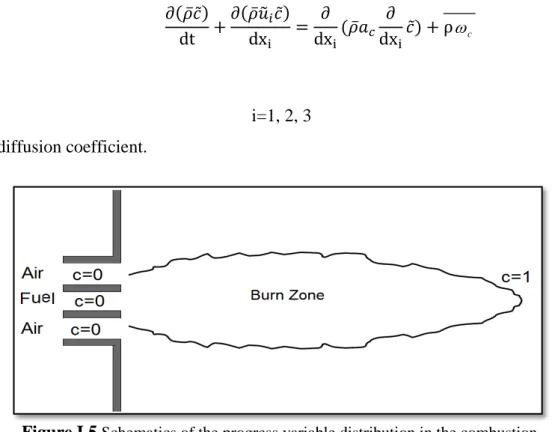
The progress variable is a combination of an intermediate and a product species. The progress variable is better interpreted as a step function that separates unburnt mixture and burnt gas in a given flow field (figure I.5). It is therefore related to the spatial structure of the flame front and its statistics rather than to a reacting scalar such as the temperature or the reactants and products. Turbulent closure of the source term of the progress variable is based on a model for the turbulent flame rate. This property of c becomes more evident when the PDF of c at a given location x is considered. It is introduced as [43, 44, 57, 58]:

𝑐 = 𝑇 − 𝑇0

𝑇_𝑒𝑞− 𝑇₀ (I.51) The progress variable c is defined as a normalized product mass fraction [44]:

𝑐 = 𝑌𝑝

(30)

It is possible to make combinations between the chemical species:

𝑐 = 𝑌𝑝1+ 𝑌𝑝2

𝑌_𝑝1𝑒𝑞+ 𝑌_𝑝2𝑒𝑞 (I.53) Where Y is the mass fraction of productions. _P

The transport equation gives the progress variable c may be in the form [54, 59]: ∂(𝜌̅𝑐̃) dt + ∂(𝜌̅𝑢̃𝑖𝑐̃) dx_i = ∂ dx_i(𝜌̅𝑎𝑐 ∂ dx_i𝑐̃) + ρc ̅̅̅̅̅̅ _(I.54) Where: i=1, 2, 3 𝑎_𝑐 is the diffusion coefficient.

Figure I.5 Schematics of the progress variable distribution in the combustion.

I.4.5 Mixture Fraction Equation

The role of mixture fraction in non-premixed combustion is the description of the transport of conserved scalars parameters based on the inflow mixing streams The mixture fraction is a conserved scalar variable, which means that a conservation equation for the mixture fraction will have no source term. The basis of the non-premixed modeling approach is that under a certain set of simplifying assumptions, the instantaneous thermo-chemical state of the fluid is related to a conserved scalar quantity known as the mixture fraction(Z) [47, 55, 60].

Conservation equations can be reduced to the solution of a single transport equation for the mixture fraction. All the species mass fractions and temperature can then be calculated from mixture fraction concentrations using functional relationships. This forms the basis of the conserved scalar approach [28,44, 48, 49].

(31)

∂(𝜌̅𝑍̃) ∂t + ∂(𝜌̅𝑢̃_𝑖𝑍̃) ∂x_i = ∂ ∂x_i(𝜌̅𝑎𝑐 ∂𝑍̃ ∂x_i) (I.55) With: i=1,2,3

This scalar is passive, there are no source terms of chemical reaction, the first term of left border of equation is unsteady and the second is the convection. The right border represented the molecular diffusion [44, 49, 53].

Figure I.6 Surface of stoichiometric mixture (Zst) for a turbulent jet diffusion flame [28].

Conclusion

In this chapter, we dealt with the idea for turbulent non-premixed combustion modeling. Where, the turbulence is a complicate status of flows that needs to precede a new methods and models to resolve the problem in this flow status. The considering of the combustion complicates more system. For this reason, we use LES to describe the turbulence by statistical methods in the Navier-Stokes equations to describe correctly the structure of turbulent flows. In LES, the effects of the small turbulent motions are modeled, and the larger ones are computed. The PDF methods are used to resolve the closure problem in the thermo-chemical terms in the governing equations of turbulent combustion.

(32)

C

H

_H

A

_A

P

_P

T

_T

E

_E

R

_R

I

_I

I

_I

N

(33)

omputational Fluid Dynamics codes play an important role in the design and the optimization of the flows processes. CFDs are created by the numerical methods for the solutions of the set of governing equations describing the system. Also, they are given as tools to present the details that the experimental can’t give. The combustion process is described by the set equations that govern the transport equations for the fluid dynamics, the heat transfer and the chemical reactions. Moreover, the details of the flow are added in the CFD considering the combustion case with chemical multispecies and with multi-scales of flow.

The aim of this chapter is to give the main steps of the simulation and the modeling of the combustion of the two types of the flues (Methane and Bio fuel): configuration, meshes, equations ...

II.1 Computational Fluid Dynamics

A Computational Fluid Dynamics (CFD) is a tool, that we can use to study the fluid behavior accompanied with chemical reaction, heat transfer and mass transfer. The computer science progress has an impact on the CFD efficiency with the integration of the complex equations: conservation of mass, momentum, energy and chemical species [61, 62, 63, 64]:

 Meshing the geometry.

 Applying the governing equations on the cells of the computational domain.

 Using the algebraic form of equations.

The common steps in the CFD applications can be summarized in the Figure II.1.

Figure II.1 Flow chart general CFD methodology[65 ].

C

H

A

P

T

E

R

I

N

u

m

e

r

i

c

a

l

S

t

u

d

y

o

f

C

o

m

b

u

s

t

i

o

n

b

y

C

F

D

(34)

II.2 Fluent CFD

To do this, we use a software package, it includes three major components:

FLUENT

&

GAMBIT

&

Exeed

In this research, FLUENT 6.3.26 software is used to achieve the modeling and simulation. The pre-processor used to construct the model grid is GAMBIT 2.2.30.

II.2.1GAMBIT

GAMBIT software is used for the illustration of the configuration and establishing the pre-processing phase of modeling i.e. drawing the model (for geometry modeling and mesh generation), constructing the grid and defining the boundaries and zones. GAMBIT was designed to help in analyzing and designing of mesh building models for CFD and other scientific applications. GAMBIT receives user input primarily by means of its graphical user interface (GUI) [56, 66].

II.2.2 FLUENT

FLUENT is one of the widely used CFD software package. Which is designed for numerical simulations of various kinds of flows. Furthermore, it treats the problem and then gives the result [64].

II.2.3 EXEED

EXEED execute GAMBIT (which is designed for Linux system) in the Windows system.

II.3 Steps for CFD Analysis

II.3.1 Step 01: Creating And Meshing Basic Geometry

This step illustrates geometry creation and mesh generation for a simple geometry using GAMBIT. The most important elements of GAMBIT for drawing the combustion chamber is the row of three buttons at the top right to control the various operations (figure II.2):

(35)

(1) Geometry: Used to create various two and three-dimensional shapes for the problem.

(2) Mesh: Used to mesh the geometry into smaller areas/volumes for use in numerical solution methods.

(3) Zones: Used to define boundaries and continuum types.

Figure II.2 Combustion chamber design by GAMBIT.

II.3.2 Step 02: Opening FLUENT

Start the 3DDP (three-dimensional double precision) version of FLUENT.

3ddp → Run

(36)

II.3.3 Step 03: Grid

1. Read the Case file

File → Read → Case

Go to the directory where you saved your mesh file is saved and open the file with extension .msh.

2. Check the grid

Grid → Check

 For further confirmation, under the Display menu choose Grid. This will open the Grid Display window.

 Click on the Display icon.

3. Scale the grid

Grid → scale

 Under units conversion, select cm from the drop-down list to complete the phrase "Grid was created in cm".

 Click Scale to scale the grid. The reported values of the Domain Extents will be reported in the default SI units of meters.

4. Display of grid

(37)

 Retain the default settings.

 Click Display to view the grid in the graphics display window (Figure II.5).

Figure II.5 Graphic Display of Grid.

II.3.4 Step 04: Define Solver Properties

1. Retain the default solver settings

Define → Models → Solver

Define the domain as axisymmetric, and keep the default (segregated) solver. 2. Enable heat transfer by activating the energy equation:

Define → Models → Energy

Figure II.6 Energy Equation solution.

The energy equation needs to be turned on since this is a compressible flow where the energy equation is coupled to the continuity and momentum equations.

3. Select the standard LES turbulence model:

Define → Models → Viscous

4. Select the P1 radiation model:

(38)

5.Select the Non-Premixed Combustion model:

Define → Models → Species → Transport & Reaction

Figure II.7 Definition of Transport & Reaction model.

 Under Model, select Non-Premixed Combustion.

 Under PDF Options, turn on Inlet Diffusion.

 In the Mixture Material drop-down list under PDF-mixture.

II.3.5 Step 05: Define Material Properties

II.3.5.1 Mixture Materials

The concept of mixture materials has been implemented in FLUENT to facilitate the setup of species transport and reacting flow. A mixture material may be thought as a set of species and a list of rules governing their interaction. The mixture material carries with it the following information:

 A list of the constituent species, referred to as “fluid” materials

 A list of mixing laws dictating how mixture properties (density, viscosity, specific heat, etc.) are to be derived from the properties of individual species if composition dependent properties are desired

 A direct specification of mixture properties if composition-independent properties are desired

 Diffusion coefficients for individual species in the mixture

 Other material properties (absorption and scattering coefficients) that are not associated with individual species.

(39)

Define material properties for heat transfer:

Define → Materials

Figure II.8 Materials Window.

II.3.6 Step 06: Define Boundary Conditions

Set boundary conditions for the following surfaces: inlet, outlet, wall …

Boundary conditions must be properly specified. Either over- or under specifying boundary conditions will lead to an inaccurate solution. A proper formulation requires [68]:

 governing equations.

 boundary conditions.

 coordinate system specification.

Define the boundary conditions for the zones (Figure II.9):

(40)

Figure II.9 Boundary conditions of wall temperature.

 Select wall from the Zone list.

 Select wall from the Type list.

 Click the Thermal tab.

 Select Temperature from the Thermal Conditions list.

 Enter 500 K for Temperature.

 Enter 1 for Internal Emissivity.

 Click OK to close the Wall panel.

II.3.7 Step 07: Non Adiabatic PDF Table

1. Select the Non-Premixed Combustion model.

(41)

 Select Create Table.

 Click the Boundary tab to add and define the boundary species (Figure II.11).

Figure II.11 Mean temperature as function for average mixture fraction.

 Click the Table tab to specify the table parameters and calculate the PDF table.

 Click the display Table… button to open the PDF Table dialog box.

 click display,we get the following (Figure II.12):

(42)

II.3.8 Step 08: Solution

1. Set Solution Controls.

Solve → Controls → Solution

The default under-relaxation factors are considered to be too aggressive for reacting flow cases with high swirl velocity. For a combustion model it may be necessary to reduce the under-relaxation to stabilize the solution.

2.Initialize the field variables.

Solve → Initialize → Initialize

Initializing the flow using a high temperature and non-zero fuel content will allow the combustion reaction to begin. The initial condition acts as a numerical “spark” to ignite the Bio fuel air mixture.

3. Enable the display of residuals during the solution process.

Solve → Monitors → Residual

4. Write case (---.cas)

File → Write → Case

5. Iterate Until Convergence

Solve → Iterate

Enter a value of 0.0002 for the Time Step Size and enter 1000 under Number of time steps. Increase the Maximum Iterations per Time Step to 300. Click Iterate (Figure II.13).

(43)

6. Save the data file (---.dat).

File → Write → Data

II.3.9 Step 09: Analyze Results

II.3.9.1 Display Contour & Vectors

a) Temperature:

Display the predicted temperature field:

Display → contours

Figure II.14 Display Contour.

 Select Temperature...

 Select Total Temperature from the Contours of drop-down lists.

 Select z = 0.

(44)

Figure II.15 Total temperature contours of Biofuel/Air.

b) CO Mass fraction:

Display the predicted CO Mass fraction

Figure II.16 CO Mass Fraction Contours of Biofuel/Air..

c) Velocity:

Display Contour of Velocity

(45)

Figure II.17 X Velocity Contours of Biofuel/Air.

II.3.9.2 Drawing the graphs

Plot → XY Plot

Figure II.18 Solution XY Plot panel.

 Select Temperature...

 Select Total Temperature from the Contours of drop-down lists.

 Select surfaces from the Surfaces selection list or File Data.

(46)

Figure II.19 Plot of Total Temperature.

Conclusion

In the present study, CFD simulation tools are shown and used to investigate and to understand the Bio fuel combustion. CFD is introduced as an important tool to study and to simulate the cylindrical combustion chamber in three-dimensional supplied by the Bio fuel. Moreover, the combustion modeling is carried out by the dynamic model of turbulence Large Eddy Simulation (LES) coupled with scalar approach β-PDF including in FLUENT. In the next chapter we will discuss the obtained results and compare them with the experience.

(47)

C

H

_H

A

_A

P

_P

T

_T

E

_E

R

_R

I

_I

I

_I

I

_I

R

(48)

he objective of this chapter is the computation and the interpretation of the results obtained by FLUENT-CFD code for three dimensional the non-premixed turbulent combustion in cylindrical chamber supplied by two coaxial jets (Biofue/air or Methane/air). Also, in this part we validate the performance of the LES-WALE model coupled with the Beta-PDF approach with the experimental data in the same stations and the same conditions.

III.1 Experimental Configuration and Application Domain

III.1.1 The Experimental Configuration

The configuration of the two coaxial jets that confine the combustor is given in figure III.1. Where it was the focus of numerous experimental investigations because of its relatively simple geometry and its similarity to gas turbine burner [69]. Thereby, we investigated the numerical validation of the LES/PDF coupled models with the experimental data, to study the behavior of the non-premixed combustion fueled by CH4 and Bio fuel. Whereas, the study consists of three

main parameters: mean axial velocity, mean temperature and mean mass fraction of Carbone monoxide. The cylindrical combustion chamber is of ray R4 and L in length supplied by two

coaxial jets, the central one has an internal ray R1 and an external R2, which injects the methane

with inlet mass flow rate and temperature respectively Q1 and T1. The annular one has an internal

ray R3, that injects the air with an inlet mass flow rate Q2 and preheated at a temperature T2. The

combustion chamber is pressurized to 3.8 atm and has a constant temperature wall of Twall [69].

The dimensions and ﬂow conditions speciﬁed in the experiment are summarized below: R3≡ R =0.04685 m R4=0.06115 m R1=0.03157 m R2=0.03175 m Q1 =0.0072 kg/s Q2=0.137 kg/s T1 =300 K T2 =750 K Twall =500 K L= 1m