Estimating long memory in volatility

[25] (generalized by [23]) studied partial sums and sample variance of a possibly nonzero mean stochastic volatility process with infinite variance and where the volatility is

We investigate the potential of structural changes and long memory (LM) properties in returns and volatility of the four major precious metal commodities traded on the COMEX

This model has been successfully used to capture the persistent and asymmetric dynamics of the unemployment rate, but it is not convenient for the study of the changing degree

Moreover, the model characterized by a time-varying modelling of the long memory parameter d t using a STAR process shows an upper regime characterized a long memory behavior

As is seen, the estimated model captures both short and long memory dy- namics in the mean-reverting behavior of the unemployment rate to its long-run value.. These results hold

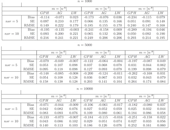
In this paper we perform a Monte Carlo study based on three well-known semiparametric estimates for the long memory fractional parameter. We study the efficiency of Geweke

In Experiment 1b, we manipulated semantic relatedness in immediate serial recall tasks with or without an interfering task by presenting lists of six words that

This choice of k depends on the smoothness parameter β, and since it is not of the same order as the optimal values of k for the loss l(f, f ′ ) on the spectral densities, the