Real Time DC Motor Speed Control Based on Labview interfaced with Arduino
Texte intégral
Figure
![Figure 1 DC motor constraction [15]](https://thumb-eu.123doks.com/thumbv2/123doknet/12228601.318183/11.892.219.704.790.1070/figure-dc-motor-constraction.webp)

![Figure 4 Equivalent circuit of a SEDC machine. [4].](https://thumb-eu.123doks.com/thumbv2/123doknet/12228601.318183/13.892.202.740.354.544/figure-equivalent-circuit-sedc-machine.webp)
![Figure 5 Equivalent circuit for separate field and armature excitation [4]](https://thumb-eu.123doks.com/thumbv2/123doknet/12228601.318183/14.892.198.749.211.363/figure-equivalent-circuit-for-separate-field-armature-excitation.webp)


![Figure 9 Simplifed Buck Converter Circuit Diagram [5]](https://thumb-eu.123doks.com/thumbv2/123doknet/12228601.318183/19.892.288.665.401.609/figure-simplifed-buck-converter-circuit-diagram.webp)
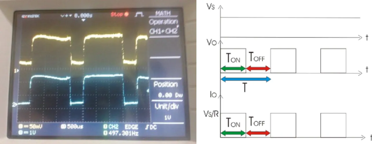
![Figure 12 Operation of Buck Converter with Resistive Load [9]](https://thumb-eu.123doks.com/thumbv2/123doknet/12228601.318183/20.892.303.634.371.574/figure-operation-buck-converter-resistive-load.webp)
Documents relatifs
Inside the "cage" at the M-42 building is another set of controls, (Figure 3), There is a button for starting the fans, a button for starting the flaps for frequency
2 ةساردلا هذى جئاتن : ةيرادلإا تايلمعلا ةسدنى ةداعإ قيبطت بولسأ مادختسا نإ ( ةردنلذا ) اضرلا ىوتسم ةدايز لىإ يدؤي ةيرادلإا متهايوتسم ةفاك في
The interviews included all six of the staff members of CLU as February 2010; eight staff at member organizations of CLU or the CLU-convened Green Justice Coalition (including
Unité Mixte de Recherche Contrôle des Maladies Animales Exotiques et Emergentes, Centre de Coopération Internationale en Recherche Agronomique pour le Développement (CIRAD),
The existence of a minimum time below which it is impossible to descend, necessarily implies the existence of a maximum speed: in fact, if ad absurdum it
La jurisprudence admet la possibilité d’inclure le salaire afférent aux vacances dans le salaire courant en cas de travail irrégulier à deux conditions formelles cumulatives :
A Practical Scheme for Induction Motor Speed Sensorless Field Oriented Control.. Abdessalam Makouf, Mohamed Benbouzid, Demba Diallo,
We show that the Tolman-Ehrenfest effect (in a stationary gravitational field, temperature is not constant in space at thermal equilibrium) can be derived very simply by applying
