Energy Efficient Resource Allocation for Type-I HARQ Under the Rician Channel

Hence, the present work deals with the study of the dissolution mechanisms of two common vanadium compounds in 3 M sulfuric acid, at various temperatures (0 40 °C), stirring rates

Considering WPT and wireless information transfer (WIT) in different slots, we propose a time allocation scheme for optimizing the WPT time duration, power and subchannel

CDF of achievable data rates for eMBB users using slice-isolation and slice-aware resource allocation mechanisms with mixed numerologies in time domain and fixed numerology.. This

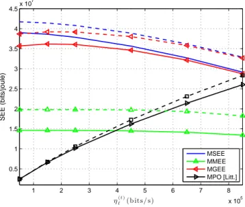
With no surprise, for both power constraints, the energy- efficient utility of the cell is higher when mobile users report their actual channel gains.. This utility increases with

In the third experiment, we run 10000 iterations of both algorithms for different amount (from C = 2 to C = 18) of available channels. For each simulation, we report in Fig. 5

Abstract—In the context of mobile clustered ad hoc networks, this paper proposes and studies a self-configuring algorithm which is able to jointly set the channel frequency and

Die syntaktische Komponente, oder Syntax, ist durch zwei große Teile gebildet: die Basis, die die Grundstrukturen, und die Umwandlungen bestimmt, die erlauben, tiefe

Scheitzer, N Daly et d’autre, Cancérologie clinique, 6eme édition,

REFERENCES

[1] X. Leturc, C. J. Le Martret, and P. Ciblat, “Energy efficient bandwidth and power allocation for Type-I HARQ under the rician channel,” in International Conference on Telecommunications (ICT), Jun. 2018.
[2] X. Leturc, P. Ciblat, and C. J. Le Martret, “Maximization of the sum of energy-efficiency for Type-I HARQ under the Rician channel,” in IEEE International Workshop on Signal Processing Advances in Wireless Communications (SPAWC), Jun. 2018.
[3] S. Marcille, P. Ciblat, and C. J. Le Martret, “Resource allocation for Type-I HARQ based wireless ad hoc networks,” IEEE Wireless Commun. Letters, vol. 1, no. 6, pp. 597–600, Dec. 2012.
[4] F. Boccardi, R. W. Heath, A. Lozano, T. L. Marzetta, and P. Popovski, “Five disruptive technology directions for 5G,” IEEE Commun. Mag., vol. 52, no. 2, pp. 74–80, Feb. 2014.
[5] M. N. Tehrani, M. Uysal, and H. Yanikomeroglu, “Device-to-device communication in 5G cellular networks: challenges, solutions, and future directions,” IEEE Commun. Mag., vol. 52, no. 5, pp. 86–92, May 2014.
[6] G. Fodor, E. Dahlman, G. Mildh, S. Parkvall, N. Reider, G. Miklós, and Z. Turányi, “Design aspects of network assisted device-to-device communications,” IEEE Commun. Mag., vol. 50, no. 3, pp. 170–177, Mar. 2012.
[7] E. Vinogradov, W. Joseph, and C. Oestges, “Measurement-based modeling of time-variant fading statistics in indoor peer-to-peer scenarios,” IEEE Trans. Antennas Propag., vol. 63, no. 5, pp. 2252–2263, May 2015.
[8] D. Tse and P. Viswanath, Fundamentals of Wireless Communication. Cambridge university press, 2005.
[9] M. K. Samimi and T. S. Rappaport, “3-D millimeter-wave statistical channel model for 5G wireless system design,” IEEE Trans. Microw. Theory Techn., vol. 64, no. 7, pp. 2207–2225, Jul. 2016.
[10] S. Sesia, I. Toufik, and M. Baker, LTE: the Long Term Evolution - From theory to practice. Wiley, 2009.
[11] C. J. Le Martret, A. Le Duc, S. Marcille, and P. Ciblat, “Analytical performance derivation of hybrid ARQ schemes at IP layer,” IEEE Trans. Commun., vol. 60, no. 5, pp. 1305–1314, May 2012.
[12] C. Y. Wong, R. S. Cheng, K. B. Letaief, and R. D. Murch, “Multiuser OFDM with adaptive subcarrier, bit, and power allocation,” IEEE J. Sel. Areas Commun., vol. 17, no. 10, pp. 1747–1758, Oct. 1999.
[13] D. T. Ngo, S. Khakurel, and T. Le-Ngoc, “Joint subchannel assignment and power allocation for OFDMA femtocell networks,” IEEE Trans. Wireless Commun., vol. 13, no. 1, pp. 342–355, Jan. 2014.
[14] A. Zappone and E. Jorswieck, “Energy efficiency in wireless networks via fractional programming theory,” Foundations and Trends in Communications and Information Theory, vol. 11, no. 3-4, pp. 185–396, 2015.
(32)
[15] D. Feng, C. Jiang, G. Lim, L. J. Cimini, G. Feng, and G. Y. Li, “A survey of energy-efficient wireless communications,” IEEE Commun. Surveys Tuts., vol. 15, no. 1, pp. 167–178, Feb. 2013.
[16] A. Chelli, E. Zedini, M. S. Alouini, J. R. Barry, and M. Pätzold, “Performance and delay analysis of hybrid ARQ with incremental redundancy over double Rayleigh fading channels,” IEEE Trans. Wireless Commun., vol. 13, no. 11, pp. 6245–6258, Nov. 2014.
[17] Y. Li, G. Ozcan, M. C. Gursoy, and S. Velipasalar, “Energy efficiency of hybrid-ARQ under statistical queuing constraints,” IEEE Trans. Commun., vol. 64, no. 10, pp. 4253–4267, Oct. 2016.
[18] I. Stanojev, O. Simeone, Y. Bar-Ness, and D. H. Kim, “Energy efficiency of non-collaborative and collaborative hybrid-ARQ protocols,” IEEE Trans. Wireless Commun., vol. 8, no. 1, pp. 326–335, Jan. 2009.
[19] T. Shafique, O. Amin, and M. S. Alouini, “Energy and spectral efficiency analysis for selective ARQ multi-channel systems,” in IEEE International Conference on Communications (ICC), May 2017, pp. 1–6.
[20] M. Jabi, M. Benjillali, L. Szczecinski, and F. Labeau, “Energy efficiency of adaptive HARQ,” IEEE Trans. Commun., vol. 64, no. 2, pp. 818–831, Feb. 2016.
[21] A. Hadjtaieb, A. Chelli, and M. S. Alouini, “Maximizing the spectral and energy efficiency of ARQ with a fixed outage probability,” in International Wireless Communications and Mobile Computing Conference (IWCMC), Aug. 2015. [22] Y. Qi, R. Hoshyar, M. A. Imran, and R. Tafazolli, “H2-ARQ-relaying: Spectrum and energy efficiency perspectives,” IEEE
J. Sel. Areas Commun., vol. 29, no. 8, pp. 1547–1558, Sep. 2011.
[23] M. Maaz, J. Lorandel, P. Mary, J.-C. Prévotet, and M. Hélard, “Energy efficiency analysis of hybrid-ARQ relay-assisted schemes in LTE-based systems,” EURASIP Journal on Wireless Communications and Networking, vol. 2016, no. 1, pp. 1–13, 2016.
[24] J. Wu, G. Wang, and Y. R. Zheng, “Energy efficiency and spectral efficiency tradeoff in Type-I ARQ systems,” IEEE J. Sel. Areas Commun., vol. 32, no. 2, pp. 356–366, Feb. 2014.
[25] G. Wang, J. Wu, and Y. R. Zheng, “Optimum energy and spectral-efficient transmissions for delay-constrained hybrid ARQ systems,” IEEE Trans. Veh. Technol., vol. 65, no. 7, pp. 5212–5221, Jul. 2016.
[26] S. Ge, Y. Xi, H. Zhao, S. Huang, and J. Wei, “Energy efficient optimization for CC-HARQ over block Rayleigh fading channels,” IEEE Commun. Letters, vol. 19, no. 10, pp. 1854–1857, Oct. 2015.
[27] F. Rosas, R. D. Souza, M. E. Pellenz, C. Oberli, G. Brante, M. Verhelst, and S. Pollin, “Optimizing the code rate of energy-constrained wireless communications with HARQ,” IEEE Trans. Wireless Commun., vol. 15, no. 1, pp. 191–205, Jan. 2016.
[28] A. Z. Ghanavati and D. Lee, “Optimizing the bit transmission power for link layer energy efficiency under imperfect CSI,” IEEE Trans. Wireless Commun., vol. 17, no. 1, pp. 29–40, Jan. 2018.
[29] E. Eraslan and B. Daneshrad, “Low-complexity link adaptation for energy efficiency maximization in MIMO-OFDM systems,” IEEE Trans. Wireless Commun., vol. 16, no. 8, pp. 5102–5114, Aug. 2017.
[30] G. Yu, Q. Chen, R. Yin, H. Zhang, and G. Y. Li, “Joint downlink and uplink resource allocation for energy-efficient carrier aggregation,” IEEE Trans. Wireless Commun., vol. 14, no. 6, pp. 3207–3218, Jun. 2015.
[31] Y. Li, M. Sheng, C. W. Tan, Y. Zhang, Y. Sun, X. Wang, Y. Shi, and J. Li, “Energy-efficient subcarrier assignment and power allocation in OFDMA systems with max-min fairness guarantees,” IEEE Trans. Commun., vol. 63, no. 9, pp. 3183–3195, Sep. 2015.
[32] L. Xu, G. Yu, and Y. Jiang, “Energy-efficient resource allocation in single-cell OFDMA systems: Multi-objective approach,” IEEE Trans. Wireless Commun., vol. 14, no. 10, pp. 5848–5858, Oct. 2015.
[33] L. Venturino, A. Zappone, C. Risi, and S. Buzzi, “Energy-efficient scheduling and power allocation in downlink OFDMA networks with base station coordination,” IEEE Trans. Wireless Commun., vol. 14, no. 1, pp. 1–14, Jan. 2015.
(33)
[34] B. Du, C. Pan, W. Zhang, and M. Chen, “Distributed energy-efficient power optimization for CoMP systems with max-min fairness,” IEEE Commun. Lett., vol. 18, no. 6, pp. 999–1002, Jun. 2014.
[35] J. Denis, M. Pischella, and D. L. Ruyet, “Energy-efficiency-based resource allocation framework for cognitive radio networks with FBMC/OFDM,” IEEE Trans. Veh. Technol., vol. 66, no. 6, pp. 4997–5013, Jun. 2017.
[36] K. G. Nguyen, L. N. Tran, O. Tervo, Q. D. Vu, and M. Juntti, “Achieving energy efficiency fairness in multicell MISO downlink,” IEEE Commun. Lett., vol. 19, no. 8, pp. 1426–1429, Aug. 2015.
[37] Y. Wu and S. Xu, “Energy-efficient multi-user resource management with IR-HARQ,” in IEEE Vehicular Technology Conference (VTC Spring), May 2012.
[38] J. Choi, J. Ha, and H. Jeon, “On the energy delay tradeoff of HARQ-IR in wireless multiuser systems,” IEEE Trans. Commun., vol. 61, no. 8, pp. 3518–3529, Aug. 2013.
[39] B. Bossy, P. Kryszkiewicz, and H. Bogucka, “Optimization of energy efficiency in the downlink LTE transmission,” in IEEE International Conference on Communications (ICC), May 2017.
[40] J. Denis, S. Smirani, B. Diomande, T. Ghariani, and B. Jouaber, “Energy-efficient coordinated beamforming for multi-cell multicast networks under statistical CSI,” in IEEE International Workshop on Signal Processing Advances in Wireless Communications (SPAWC), Jul. 2017.
[41] A. Zappone, P. Cao, and E. A. Jorswieck, “Energy efficiency optimization in relay-assisted MIMO systems with perfect and statistical CSI,” IEEE Trans. Signal Process., vol. 62, no. 2, pp. 443–457, Jan. 2014.
[42] M. Maaz, P. Mary, and M. Hélard, “Energy minimization in HARQ-I relay-assisted networks with delay-limited users,” IEEE Trans. Veh. Technol., vol. 66, no. 8, pp. 6887–6898, Aug. 2017.
[43] X. Leturc, C. J. Le Martret, and P. Ciblat, “Energy efficient resource allocation for HARQ with statistical CSI in multiuser ad hoc networks,” in IEEE International Conference on Communications (ICC), May 2017.
[44] ——, “Multiuser power and bandwidth allocation in ad hoc networks with Type-I HARQ under Rician channel with statistical CSI,” in International Conference on Military Communications and Information Systems (ICMCIS), May 2017. [45] A. Goldsmith, Wireless communications. Cambridge university press, 2005.
[46] Y. Jong, “An efficient global optimization algorithm for nonlinear sum-of-ratios problem,” 2012, [Online], Available: http://www.optimization-online.org/DB_HTML/2012/08/3586.html.
[47] W. Dinkelbach, “On nonlinear fractional programming,” Management science, vol. 13, no. 7, pp. 492–498, 1967. [48] J. Crouzeix, J. Ferland, and S. Schaible, “An algorithm for generalized fractional programs,” Journal of Optimization
Theory and Applications, vol. 47, no. 1, pp. 35–49, 1985.
[49] S. Boyd and L. Vandenberghe, Convex optimization. Cambridge university press, 2004.
[50] E. Boshkovska, D. W. K. Ng, N. Zlatanov, and R. Schober, “Practical non-linear energy harvesting model and resource allocation for SWIPT systems,” IEEE Commun. Lett., vol. 19, no. 12, pp. 2082–2085, Dec. 2015.
[51] R. Ramamonjison and V. K. Bhargava, “Energy efficiency maximization framework in cognitive downlink two-tier networks,” IEEE Trans. Wireless Commun., vol. 14, no. 3, pp. 1468–1479, Mar. 2015.
[52] D. P. Palomar and J. R. Fonollosa, “Practical algorithms for a family of waterfilling solutions,” IEEE Trans. Signal Process., vol. 53, no. 2, pp. 686–695, Feb. 2005.
Figure
Fig. 1. SEE obtained for the considered criteria versus η ` (t) , solid lines: Rayleigh channel (∀`, K ` = 0), dashed lines: Rician channel (∀`, K ` = 10).
Fig. 2. GEE obtained for the considered criteria versus η (t) ` , solid lines: Rayleigh channel (∀`, K ` = 0), dashed lines: Rician channel (∀`, K ` = 10)
Fig. 4. Gains between the Rician (∀`, K ` = 10) and the Rayleigh (∀`, K ` = 0) allocations under the Rician channel, versus η (t) ` .
Fig. 5. Gains between the Rician (∀`, K ` = 10) and the Rayleigh (∀`, K ` = 0) allocations under the Rician channel, versus the Rician K factor, with η (t) ` = 4.5 × 10 5 bits/s.
+4
Références
Documents relatifs