Efficient Optimization of the Ambiguity Functions of Multi-Static radar waveforms

HAL Id: hal-01325268

https://hal.archives-ouvertes.fr/hal-01325268

Submitted on 2 Jun 2016

HAL is a multi-disciplinary open access

archive for the deposit and dissemination of

sci-entific research documents, whether they are

pub-lished or not. The documents may come from

teaching and research institutions in France or

abroad, or from public or private research centers.

L’archive ouverte pluridisciplinaire HAL, est

destinée au dépôt et à la diffusion de documents

scientifiques de niveau recherche, publiés ou non,

émanant des établissements d’enseignement et de

recherche français ou étrangers, des laboratoires

publics ou privés.

Copyright

Efficient Optimization of the Ambiguity Functions of

Multi-Static radar waveforms

F Arlery, R Kassab, U Tan, F Lehmann

To cite this version:

F Arlery, R Kassab, U Tan, F Lehmann. Efficient Optimization of the Ambiguity Functions of

Multi-Static radar waveforms. 17th International Radar Symposium 2016 (IRS 2016), Microwave and

Radiolocation Foundation, May 2016, Cracovie, Poland. �hal-01325268�

Efficient Optimization of the Ambiguity Functions of

Multi-Static radar waveforms

F. Arlery

; R. Kassab

; U. Tan

*

THALES AIR SYSTEMS Limours, France fabien.arlery@thalesgroup.com

rami.kassab@thalesgroup.com

F. Lehmann

**

SAMOVAR, Télécom SudParis, CNRS, Université Paris-Saclay,

Evry, France

frederic.lehmann@telecom-sudparis.eu

Abstract— This paper deals with the local optimization of the

periodic or aperiodic ambiguity functions of a set of complex sequences by using a gradient method. This optimization aims to locally minimize the cross-ambiguity and the auto-ambiguity functions of a family of sequences for Multi-Static Primary Surveillance Radar (MSPSR) systems. The optimization of the ambiguity functions is done by an optimized gradient. An extension is also presented for controlling both the spectrum and the ambiguity functions.

Index Terms— Waveform design, Spectrum design, Gradient

descent, Auto-ambiguity functions, Cross-ambiguity functions, Complex sequence sets, MSPSR, MIMO.

I. INTRODUCTION

Nowadays, MSPSR systems are sustainably settled in air surveillance program [1]. Compared to mono-static radar currently in use, MSPSR system is based on a sparse network of transmitters (Tx) and receivers (Rx) (MIMO), interconnected to a Central Unit and offers advantages in terms of reliability, cost and performance.

Two kinds of MSPSR systems exist: the Passive form and the Active one. While the Passive MSPSR uses transmitters of opportunity such as radio Frequency Modulation (FM) transmitters and/or Digital Video Broadcasting-Terrestrial (DVB-T) transmitters [2], the Active MSPSR uses dedicated transmitters, which emit waveforms that are controlled and designed for a radar application. Each receiver processes the signal coming from all transmitters and reflected on the targets; and the Central Unit restores the target location by intersecting “ellipsoids” from each transmitter/ receiver pair.

Compared to a passive MSPSR, the main advantages of the active MSPSR are the use of dedicated waveforms that allow reaching better performances (like a better association of the transmitters’ contributions at the receiver level), more flexibility in the deployment of transmitters and receivers (in order to meet the requirements in localization accuracy and in horizontal and altitude coverages), and the guarantee of having a service continuity.

Although improving the radar performances by finding a sequence with an optimized ambiguity function is a common purpose, designing a set of dedicated waveforms for MSPSR systems is not an easy task.

One solution is to find easily-constructed families of sequences such as sequences of the Small Set of Kasami or other spreading codes families [3] [4]. However it can be noticed that those sequences have a good Peak to Sidelobe Level Ratio (PSLR) on the whole ambiguity function area. But in practice the Doppler frequency range can be much smaller than the bandwidth of the probing signal. For example, consider a L-band radar operating at a wavelength of 0.3 m. An airliner with a radial speed of 300 m/s gives a Doppler frequency of 2 kHz which is much smaller than the bandwidth of many MHz. Also depending on the signal duration it is not relevant to optimize the whole distance range. For example, assuming a radar instrumented range of 150 km, a pulse repetition interval of 10 ms induces an unambiguous distance range of 1500 km which is much more than the radar instrumented range of 150 km. Therefore we can confine our attention on a small area of interest defined by the maximum Doppler frequency and the radar instrumented range; we expect to obtain better sidelobe level (Fig 1.).

According to this remark, another solution is to generate a set of sequences such that the ambiguity functions are locally optimized. This kind of waveform design can be achieved by the use of cyclic algorithm, like the one introduced by Stoïca and He [5]. However this algorithm is based on the Singular Value Decompositions (SVD) of a large matrix with a complexity of O(N3) (where N is the number of elements in the

sequences).

But recent works [6] have shown the possibility to optimize the autocorrelation sidelobe energy of a single sequence by using an efficient gradient method which reduces the complexity to O(Nlog(N)). In this paper, we extend a previous approach [7] to the local optimization of the ambiguity functions of a set of aperiodic or periodic complex sequences.

Figure 1. Expected result on the ambiguity function after local optimization.

optimization area of interest

II. NOTATIONS

First, define a family set of complex sequences of length N, with

and its Doppler shift version

where and corresponds respectively to the Doppler shift and the bit time. is supposed to be a predefined waveform envelope (i.e. of constant modulus or pulsed etc.).

If we define a normalized Doppler shift ! such that "

then can be expressed as _" # %$& .

According to that, the correlation of and '_", expressed

as ( '_" ) '_", is given by: * '_" + , ) '_"-_./

0 )' 1 +

" (1) One important feature of this function is:

* '_" + * ' _2" 3+ ". 4 5!/67/89:;6<=6> ! ? @/<AB:;C6D: (2) Now let us define the partial cost function term from which we calculate the gradient:

E '_" 0 F* '_" + F GH '_{" ./} 2

. 2 I

(3) where the exponent J allows some control over the sidelobe level. When J K , E '_" corresponds to the weighted integrated sidelobe level (WISL). Otherwise, the larger the exponent, the more emphasized the dominant term is, so the gradient will essentially indicate the gradient of the PSLR. The coefficients H '_{" .} control the shape of the correlation sidelobes (H '_{" .} ? L)in the area of interest and M outside). This partial cost function term is related to the sidelobe energy within the correlation product of and '_". It corresponds to the cross-correlation between the NOP sequence and the NQOP sequence with a normalized Doppler shift !.

If we call R the set of Doppler frequencies to optimize such that:

R !S/! ? @/67/9:;6<=6> ! ? L/<AB:;C6D: (4) We can define the cost function related to sidelobe energy within the ambiguity function between and ' within the area of interest, as:

E ' 0 E '_"

"?R (5)

From that, the global cost function term from which we calculate the gradient can be expressed as the sum on E ' for each combination of sequences:

E 0 0 E '

T ' T

(6)

III. GRADIENT METHOD FOR LOCALLY OPTIMIZING THE

AMBIGUITY FUNCTIONS OF A SET OF SEQUENCES

This section provides the gradient of the global cost function, E, related to the sidelobe energy within the auto-ambiguity and cross-auto-ambiguity functions of a set of complex sequences. For calculating this ‘global’ gradient this section is divided in three parts. The first one gives the gradient equation of the cost function associated to the auto-ambiguity function of a sequence. The second part deals with the gradient calculations of the cost function within the cross-ambiguity function of a pair of sequences. And the last one combines the two previous parts and gives the ‘global’ gradient expression.

A. Optimization of the Auto-Ambiguity Function of a Sequence

This subsection provides the gradient of the cost function associated to the auto-ambiguity function of a sequence. The derivations for calculating this gradient has been done in a recent paper [7]. Therefore, for understanding and completeness, this part focuses on the key points of this calculation.

Consider the NOP -sequence of the family, the auto-ambiguity cost function is defined as:

E 0 E "

"?R (7)

where we recall that:

E " 0 F* " + F GH " ./ 2

. 2 I

(8) One can observe that the gradient of E consists of the sum of the partial gradients E _" where E _" corresponds to the cost function related to the sidelobe energy within the matched filtering response in presence of a Doppler !.

From that observation, as is a complex sequence with a predefined envelope, the partial gradient is the derivative of the cost function E _" with respect to its phase: UEN N !

UV_{N W} .

For clarity, thereafter, E _" E_" , * _" + *_" + , H " . H" . and

So, using the chain rule, it can be observed that the derivative with respect to the phase of can be done by calculating the derivatives with respect to the real and imaginary parts of :

UE! UV_W 3XN W UE! UY W 1 Y W UE! UXN W (9) As: UE" U Z [J 0 \. "]Y ^*" + _UY ^*_{U Z}" + _ 2 . 2 I 1 XN ^*" + _UXN ^*_{U Z}" + _` (10)

where \_{" .} H_{" .}F*_" + F G2 and U Z 4UY a UXN a

The partial derivatives with respect to Y _a and XN _a are given above ((11) and (12)).

Putting (11) and (12) in the chain rule equation (10) gives the equation (13).

And by defining b_" c\_{. "}d_{. 2 I}2 and e_" 4 2 f$%g . , (13) becomes: UE" UVa 3[JXN h W i^,b"j (2" ( _{- ) , j e"-_} a 1 ^,b"j ("- ) , j e")-(_ _{I 2a}kl (14)

Where m( n o 1 K 3 + _. is the reverse of m; and j p is the Hadamard product of and p.

Then, by setting: q" #^,b"j (2"( - ) , j e"-__a1 ^,b"j ("- ) , j e")-(_ _{I 2a}& a (15) r" ₄UE" UVaga (16)

The previous equation (14) can be converted to a vector form: r" _{3[JXNs j q}

"t (17)

Therefore by defining: r 4uv_u wg_a , and by taking back the original notation: r " r",

it comes from (7):

r 0 r "

"?R (22)

Finally the gradient can be expressed as a sum of correlation products that can be efficiently computed using Fast Fourier Transform (FFT). If we denote by x /y the discrete Fourier Transform operation, and according to our definition of the convolution (1) it can be derived that the convolution of two sequences m and z is equivalent to

[8]

m ) z x2 _{,/x m x z}() _{- (23)}

That gives a computation of r in { o|<}o operations.

B. Optimization of the Cross-Ambiguity Function between a Pair of Sequences

Consider now the gradient calculations of the cost function associated to the cross-ambiguity function of a pair of sequences. Here again this part still focuses on the key points of the calculation (see [7] and [9] for more details)

Let us start with the cross-ambiguity cost function between the NOP -sequence and the NQOP -sequence of the family (N ~ NQ):

E ' 0 E '_"

"?R (24)

where we recall that:

E '_" 0 F* '_" + F GH '_{" ./} 2

. 2 I

(25) Similarly to the previous subsection, as (resp. ' is a UE" UY a [J 0 \. "€Y ^*" + _ •Y • W 1 + 2 a"_{‚ 1 Y • W 3 +} a2. "_‚‚ 2 . 2 I 1 XN ^*" + _ •3XN • W 1 + 2 a" ‚ 1 XN • W 3 + a2. "‚‚ƒ (11) UE" UXN a [J 0 \. "€Y ^*" + _ •XN • W 1 + 2 a"_{‚ 1 XN • W 3 +} a2. "_‚‚ 2 . 2 I 1 XN ^*" + _ •Y • W 1 + 2 a" ‚ 3 Y • W 3 + a2. "‚‚ƒ (12) UE" UVa 3[JXN „ W … 0 \. "*2" 3+ • W 1 + 2 aI. "_‚)_{1 0 \} . "*" + • W 3 + a2. " ‚) 2 . 2 I 2 . 2 I †‡ (13) UE '_" UY , W - [J 0 \ '" .Y •* '" + ' W 1 + 2 a" ‚ 2 . 2 I (18) UE '_" UXN, W - [J 0 \ '" .XN •* '" + ' W 1 + 2 a" ‚ 2 . 2 I (19) UE '_" UY , ' W - [J 0 \ '" .Y ˆ* '" + • W 3 + a2. " ‚)‰ 2 . 2 I (20) UE '_" UXN, ' W - 3[J 0 \ '" .XN ˆ* '" + • W 3 + a2. " ‚)‰ 2 . 2 I (21)

complex sequence with a predefined envelope, the partial gradient is the derivative of the cost function E '_" with respect to its phase: UEN NŠ !

UV_{N W} (resp./ uv _{' $}

u _{' w} .

According to the chain rule equation again, we focus our attention to the partial derivatives with respect to Y , _a- and XN, a- (resp. /Y , '_a- and XN, '_a- and we obtain equations (18) and (19) (resp. (20) and (21)), where \ '_{" .} H '_{" .}F* '_" + F G2 .

Putting (18) and (19) (resp. (20) and (21)) in the chain rule equation (10) gives (26) (resp. (27)).

And by defining b '_" c\ '_{" .}d . 2 I

2

and e_" 4 2 f$%g

. , equations (26) and (27) become: UE '_" UV W 3[JXN € W •^b '"j ((' _2"_ ) , 'j e_"-‚ aƒ (28) UE '_" UV ' W 3[JXN i ' W ^,b '"j ( '" -) , 'j e_")-(_ I 2ak (29) By noting: r '" 4uv_u ' $_a g a , r ' '_" 4uv_{u '}' $_a g a , q‹ '_" 4•^b '_"j ((' _2"_ ) , 'j e_"-‚ ag_a , qŒ '_" #^,b '_"j ( '_"- ) , 'j e_")-(_ I 2a&_a , the previous equations can be converted to a vector form:

r '" 3[JXNi j q‹ '_"k (30) r ' '" 3[JXNi 'j qŒ '_"k (31) And by defining: r ' 4uv_u ' wg_a and: r ' ' 4uv_u ' ' wg_a it comes from equation (7):

r ' 0 r '"

"?R (32)

r ' ' 0 r ' '"

"?R (33)

Similarly to the previous section, the gradient consists of a sum of correlation products that can be efficiently computed using Fast Fourier Transforms (FFT) [8].

So the computation of r 'and r ' ' can be done in { o•Ž•o operations.

C. Global Gradient Calculations

From that, the two previous subsections are combined for calculating de ‘global’ gradient.

Given that: E 0 0 E T T (34) It comes: UE UV W 0 0 UEUV W T T (35) Finally, converted in vector form the equation (35) becomes:

r 0 0 r T T / 0 r ' T ' '_• 1 0 r ' T ' '_• 1 r (36) where: r #_u uv_a& a .

IV. GRADIENT METHOD FOR CONTROLING THE OUT-OF-BAND

FREQUENCIES

This section provides the gradient of the cost function related to the out-of-band spectrum energy of a sequence.

First, define a complex sequence , and its Fourier transform ‘’ “” ! _{" •}’2 over o’ – o elements (zero-padding).

“” ! 0 + 2 ."’

’2 . •

(37) If we define the out-of-band spectrum energy as the cost function term to minimize, it comes:

EQ _{0F“” ! F} G' ’2 " • H"Q (38) UE '_" UV W 3[JXN „ W 0 \ '" .* ' 2" 3+ • ' W 1 + 2 aI. " ‚) 2 . 2 I ‡ (26) UE '_" UV ' W 3[JXN „ ' W 0 \ '" .* '" + • W 3 + a2. " ‚) 2 . 2 I ‡ (27)

where H_"Q control the shape of the out-of-band emissions (the area of interest).

Similarly to the previous section, as is a complex sequence with a predefined envelope, the gradient is the derivative of the out-of-band cost function EQ with respect to its phase: _uuv'

w. Following the same approach as the one described in the previous section, the gradient is given by:

UEQ UVa 3[J Q_{XN ] W 0 \} "“”) ! 2 a" ’ ’2 " • ` (39) where: \_"Q H_"QF“” ! F ,G'2 -. By defining bQ c\_"Qd_{" 2 I}2 , ‘’ “” ! _{" •}’2 , and x’ /y the Discrete Fourier Transform (DFT) over o’ elements, it comes that the gradient vector, rQ #uv_u '

w&_a is given by: rQ _3[JQ_{XNs j x’,b}Q_{j ‘’})_{-t (40)} Here again, it is obvious that the computation of rQcan be done in { o|<}o operations.

V. APPLICATIONS

This section provides some applications of those methods such as:

- The design of a set of sequences that optimizes the ambiguity functions in aperiodic and periodic case. - And the design of a set of sequences that optimizes

both the ambiguity functions and the out-of-band spectrum rejection in aperiodic and periodic case.

A. Optimizing the ambiguity functions of a set of polyphase sequences

The following examples show the sidelobe rejection that can be obtained by an iterative application of (36).

A random family of complex sequences is generated as a starting point for the algorithm. Then a gradient descent is done by simply adjusting the descent step — during the process. The process continues until an exit criterion is met (an upper limit on the number of iterations, or a lower threshold on the minimum improvement acceptable between two successive iterations).

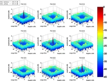
Figures (2), (3), (4) and (5) show the improvement after optimizing the ambiguity functions (R ˜3™š ™›) of a set of ™ complex sequences (of length o KM[œ) in different configurations:

- with a local weighting ( H '_{. "} K W S+S • žœ/ŽŸ *HW¡ /M 5 ! N NQ _);

- with a constant weighting

(H '_{. "} K 5 + ! N NQ );

with a large exponent (J œ ) and in both aperiodic and periodic case.

Figure 2. Ambiguity functions obtained with a local weighting in the periodic case.

Figure 3. Ambiguity functions obtained with a local weighting in the aperiodic case.

Figure 4. Ambiguity functions obtained with a constant weighting in the periodic case.

Figure 5. Ambiguity functions obtained with a constant weighting in the aperiodic case.

The algorithm well-improves the PSLR in the area of interest. For comparison, the PSLR of a sequence from the Small Set of Kasami is about [¢£o/, i.e. about 3[œ/¤¥ for a sequence of 1024 elements [4]. So even compared to those easily-constructed sequences, it gives better results.

Moreover, this algorithm is highly faster than the cyclic algorithms introduced in [5]. This is due to the efficient gradient calculations ({ o•<}o ) whereas cyclic algorithms are based on a SVD operation (O(N3)) on each iteration.

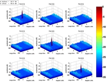
Figure 6. Ambiguity functions obtained with a local weighting in the aperiodic case.

Figure 7. Spectrums obtained with local weighting in the aperiodic case.

B. Optimizing both the ambiguity functions of a set of polyphase sequences and the out-of-band rejection

This example shows the sidelobe and out-of-band rejections possible by iterative application of (36) and (40). Here, we follow the same process as the one described in the previous examples. Except that in this case, the gradient is given by ¦r 1 K 3 ¦ rQ _{, where r}Q _{is the out-of-band gradient} vector of the NOP-sequence (Cf. (40)) and ¦ ? §Mš K¨.

Figures (6) and (7) show the result of the optimization in the following configuration: ™ , o KM[œ , R ˜3™š ™› , H '_{. "} K W S+S • žœ/<therwise/M 5 ! N NQ , J œ , o’ [o [Mœ© , H"Q K W ! ª o/<AB:;C6D:/M , JQ œ , in the aperiodic case.

It can be observed that the algorithm still improves the PSLR. The gain may be lower than in the previous case, but, the spectrum is here controlled.

VI. CONCLUSION

In this paper, new gradient methods for optimizing the ambiguity functions of a set of complex sequences were derived.

We have shown that the gradient for optimizing the ambiguity functions is based on simple operations that can be performed using FFT. The result is that the gradient can be computed with O(Nlog(N)) operations. This important result offers the possibility to optimize quite long sequences with relatively a short time of computation compared to existing methods. We have also shown that the gradient for optimizing the out-of-band emissions of a complex sequences is based on DFT operations, that can be fast computed by means of FFT. Finally, by combining both gradients we have designed a set of sequences with interesting properties for radar applications: a low PSLR and a good out-of-band rejection.

REFERENCES

[1] «Surveillance developments in SESAR» (https://www.eurocontrol.int/articles/surveillance-developments-sesar) [2] N. Millet and M. Klein, «Multi Receiver Passive Radar Tracking,» IEEE

Transactions on Aerospace and Electronic Systems, Vol. 27, No. 10,

2012.

[3] F. Arlery, M. Klein and F. Lehmann, «Utilization of Spreading Codes as dedicated waveforms for Active Multi-Static Primary Surveillance Radar,» IEEE Radar Symposium (IRS), pp. 327-332, 2015.

[4] D. V. Sarwate and M. B. Pursley, «Crosscorrelation properties of pseudorandom and related sequences,» Proceeding of the IEEE, vol. 68, pp. 593-619, May 1980.

[5] H. He, J. Li and P. Stoica, «Waveform Design for Active Sensing Systems : A Computational Approach,» New York: Cambridge University Press, 2012.

[6] J. M. Baden, M. S. Davis and L. Schmieder, «Efficient Energy Gradient Calculations for Binary and Complex Sequences,» IEEE Radar

Conference (RadarCon), pp. 301-309, Mai 2015.

[7] F. Arlery, R. Kassab, U. Tan and F. Lehmann, «Efficient Gradient Method for Locally Optimizing the Periodic/Aperiodic Ambiguity Function,» IEEE Radar Conference (RadarCon), , 2015. ‘in press’ [8] R. N. Bracewell, «The Fourier Transform and its Applications,» 3rd

Edition éd., New York: McGraw-Hill, 1986.

[9] U. Tan, C. Adnet, O. Rabaste, J.-P. Ovarlez and J.-P. Guyvarch, «Phase Code Optimization for coherent MIMO Radar via Gradient Descent,»