Mind the Portability: A Warriors Guide through Realistic Profiled Side-channel Analysis

HAL Id: hal-03065836

https://hal.inria.fr/hal-03065836

Submitted on 15 Dec 2020

HAL is a multi-disciplinary open access

archive for the deposit and dissemination of

sci-entific research documents, whether they are

pub-lished or not. The documents may come from

teaching and research institutions in France or

abroad, or from public or private research centers.

L’archive ouverte pluridisciplinaire HAL, est

destinée au dépôt et à la diffusion de documents

scientifiques de niveau recherche, publiés ou non,

émanant des établissements d’enseignement et de

recherche français ou étrangers, des laboratoires

publics ou privés.

Mind the Portability: A Warriors Guide through

Realistic Profiled Side-channel Analysis

Shivam Bhasin, Anupam Chattopadhyay, Annelie Heuser, Dirmanto Jap,

Stjepan Picek, Ritu Ranjan

To cite this version:

Shivam Bhasin, Anupam Chattopadhyay, Annelie Heuser, Dirmanto Jap, Stjepan Picek, et al.. Mind

the Portability: A Warriors Guide through Realistic Profiled Sidechannel Analysis. NDSS 2020

-Network and Distributed System Security Symposium, Feb 2020, San Diego, United States. pp.1-14,

�10.14722/ndss.2020.24390�. �hal-03065836�

Mind the Portability: A Warriors Guide through

Realistic Profiled Side-channel Analysis

Shivam Bhasin

Nanyang Technological University Singapore

Email: sbhasin@ntu.edu.sg

Dirmanto Jap

Nanyang Technological University Singapore

Email: djap@ntu.edu.sg

Anupam Chattopadhyay

Nanyang Technological University Singapore

Email: anupam@ntu.edu.sg

Stjepan Picek

Delft University of Technology The Netherlands Email: s.picek@tudelft.nl

Annelie Heuser

Univ Rennes, Inria, CNRS, IRISA France

Email: annelie.heuser@irisa.fr

Ritu Ranjan Shrivastwa

Secure-IC France

Email: rituranjan@secure-ic.com

Abstract—Profiled side-channel attacks represent a practical threat to digital devices, thereby having the potential to disrupt the foundation of e-commerce, the Internet of Things (IoT), and smart cities. In the profiled side-channel attack, the adversary gains knowledge about the target device by getting access to a cloned device. Though these two devices are different in real-world scenarios, yet, unfortunately, a large part of research works simplifies the setting by using only a single device for both pro-filing and attacking. There, the portability issue is conveniently ignored to ease the experimental procedure. In parallel to the above developments, machine learning techniques are used in recent literature, demonstrating excellent performance in profiled side-channel attacks. Again, unfortunately, the portability is neglected.

In this paper, we consider realistic side-channel scenarios and commonly used machine learning techniques to evaluate the influ-ence of portability on the efficacy of an attack. Our experimental results show that portability plays an important role and should not be disregarded as it contributes to a significant overestimate of the attack efficiency, which can easily be an order of magnitude size. After establishing the importance of portability, we propose a new model called the Multiple Device Model (MDM) that formally incorporates the device to device variation during a profiled side-channel attack. We show through experimental studies how machine learning and MDM significantly enhance the capacity for practical side-channel attacks. More precisely, we demonstrate how MDM can improve the performance of an attack by order of magnitude, completely negating the influence of portability.

I. INTRODUCTION

Modern digital systems, ranging from high-performance servers to ultra-lightweight microcontrollers, are universally equipped with cryptographic primitives, which act as the foundation of security, trust, and privacy protocols. Though these primitives are proven to be mathematically secure, poor

implementation choices can make them vulnerable to even an unsophisticated attacker. A range of such vulnerabilities are commonly known as side-channel leakage [1], which exploits various sources of information leakage in the device. Such leakages could be in the form of timing [2], power [3], elec-tromagnetic (EM) emanation [4], speculative executions [5], remote on-chip monitoring [6], etc. Different side-channel attacks (SCA) have been proposed over the last two decades to exploit these physical leakages. In this work, we focus on power/EM side-channel attacks targeting secret key recovery from cryptographic algorithms.

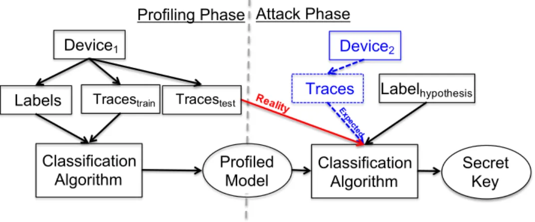
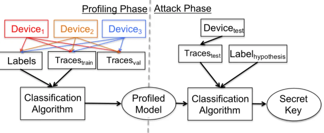
In SCA, profiled-based attacks are considered as one of the strongest possible attacks [7]. The strength of profiled-based attacks arises from their capability to fully characterize the device. There, the attacker has full control over a clone device, which can be used to build its complete profile. This profile is then used by the attacker to target other similar devices to recover the secret information. An illustration of profiled SCA is shown in Figure 1. The most common profiled SCA is template attack [7], which profiles model with mean and standard deviation. After the profiling phase, the attacker would ideally need only a single measurement in the attack phase to break the implementation. Performing such an attack enables a worst-case security evaluation.

1) Expectation vs Reality: In an ideal setting, the device for profiling and testing are different. Still, most of the works in existing literature do not consider multiple devices but profile and test the same device [8] (see Figure 1 and the difference between reality and expected cases). Consequently, despite the common perception about the practicality of SCA, a large body of results comes from unrealistic experimental settings. Indeed, the presence of process variation or different acquisition methods [9], [10] may cause a successful “single-device-model” attack to fail. In [11], authors perform a tem-plate attack on AES encryption in a wireless keyboard. They report 28% success on a different keyboard as compared to 100% when profiling and testing on the same keyboard. This issue is popularly known as portability, where we consider

Network and Distributed Systems Security (NDSS) Symposium 2020 23-26 February 2020, San Diego, CA, USA

ISBN 1-891562-61-4

Device

Labels

Classification

Algorithm

Device

Traces

Label

Classification

Algorithm

Secret

Key

Profiled

Model

Profiling Phase Attack Phase

Tracestest

Fig. 1: Illustration of profiled side-channel attacks highlighting the actual case and the usual practice in the literature. While template attacks were used as a classification algorithm in the past, adoption of machine learning has been the recent trend. Note how the measurements to attack are commonly obtained from the same device as the measurements to build the model while disregarding the requirement to use a different attack device.

all effects due to different devices and keys between profiled device and device under attack.

Definition 1: Let us denote the device under attack (target) as B and a similar or clone device as ˆB, where the differences between B and ˆB are due to uncontrolled variations in process, measurement setup, or other stochastic factors ˆP . Portability denotes all settings in which an attacker can conduct the training on the measurement data obtained from a clone device

ˆ

B and import the learned knowledge L_Bˆ to model the actual

device under target B, under similar parameter setup P . A. Machine Learning-based SCA

Recently, machine learning techniques have soared in pop-ularity in the side-channel community [12], [13]. There, the supervised learning paradigm can be considered similar to profiled-based methods used in side-channel attacks. Consid-ering Figure 1, a machine learning algorithm replaces template attacks as a classification algorithm.

It has been shown that machine learning techniques could perform better than classical profiled side-channel attacks [13]. The researchers first started with simpler machine learning techniques like Random Forest and Support Vector Machines and targets without countermeasures [14], [15], [16], [17], [18]. Already these results suggested machine learning to be very powerful, especially in settings where the training phase was limited, i.e., the attacker had a relatively small number of measurements to profile. More recently, researchers also started using deep learning, most notably multilayer perceptron (MLP) and convolutional neural networks (CNN). Such ob-tained results surpassed simpler machine learning techniques but also showed remarkable performance on targets protected with countermeasures [12], [13], [19], [20], [21], [22]. As an example, Kim et al. used deep learning (convolutional neural networks) to break a target protected with the random delay countermeasure with only three measurements in the attack phase [23].

However, the portability aspect of machine learning-based SCA, or rather SCA in general, is not properly explored. These factors are also not well captured in standard SCA metrics like Normalized Inter-Class Variance (NICV [24]). As shown later, training and testing traces with similar NICV can have very different attack performance. In this paper, we conduct a detailed analysis of portability issues arising in profiled side-channel attacks. We start by first establishing a baseline case, which represents the scenario mostly used in related works where both profiling and attacking is done on the same device and using the same secret key. Later, we explore different settings that would turn up in a realistic profiled SCA, considering scenarios with separate keys and devices. We show that this case can be orders of magnitude more difficult than the scenario where one device is used and thus undermining the security of the target due to poor assumptions. As shown later with experimental data, the best attack in the hardest setting with different devices and keys needs > 20× more samples for a successful attack, when compared to a similar attack in the easiest setting of the same device and key, clearly highlighting the issue of portability. We identify that one of the key points is how the validation procedure is performed. To tackle this problem, we propose a new model of how to conduct training, validation, and testing, which we call the Multiple Device Model. We then experimentally show that this model can help assess and improve the realistic attack efficiency in practical settings. The proposed model applies to both profiled SCA with and without the usage of machine learning.

B. Contributions

The main contributions of this work are:

1) We conduct a detailed analysis of portability issues con-sidering four different portability scenarios and state-of-the-art machine learning techniques. We show that the realistic setting with different devices and keys in pro-filing and attacking phases is significantly more difficult

than the commonly explored setting where a single device and key is used for both profiling and attack. As far as we are aware, such an analysis has not been done before. 2) We highlight that a large part of the difficulty when considering a portability scenario arises due to a sub-optimal validation phase.

3) We propose a new model for profiled SCAs called the Multiple Device Model (MDM). We show this model is able to cope with validation problems better and, conse-quently, achieve significantly better attack performance. We emphasize that the training data for SCA is closely linked to the device properties, which means that device-to-device variation has a major role.

4) We show how portability issues also arise when consider-ing the EM side-channel and probe placconsider-ing by human op-erators. Subsequently, we demonstrate how MDM helps the performance in such a scenario.

To the best of our knowledge, this is the most comprehen-sive study on portability for side-channel attacks, uncovering multiple new insights and techniques.

The rest of this paper is organized as follows. In Section II, we briefly discuss the profiled side-channel analysis. After-ward, we introduce machine learning techniques we use in this paper and provide a short discussion on validation and cross-validation techniques. Section III discusses the threat model, hyper-parameter tuning, experimental setup, and four scenarios we investigate. In Section IV, we give results for our experiments and provide some general observations. In Section V, we discuss the validation phase and the possibility of overfitting and underfitting. Afterward, we introduce the new model for profiled side-channel attacks. Section VI dis-cusses the portability scenarios arising from human errors in the positioning of EM probes. Finally, in Section VIII, we conclude the paper and provide several possible future research directions.

II. BACKGROUND

In this section, we start by providing information about profiled side-channel analysis. Then, we discuss machine learning algorithms we use in our experiments and differences between validation and cross-validation procedures.

A. Profiled Side-channel Analysis

Side-channel attacks use implementation related leakages to mount an attack [3]. In the context of cryptography, they target physical leakage from the insecure implementation of otherwise theoretically secure cryptographic algorithms. In this work, we focus on the most basic but still strong leakage source, i.e., power/EM leakage.

Profiled channel attacks are the strongest type of side-channel attacks as they assume an adversary with access to a clone device. In the present context, the adversary can control all the inputs, such as random plaintexts and key, to the clone device and observe the corresponding leakage. The adversary collects only a few traces from the attack device with an unknown secret key. By comparing the attack traces with the

characterized model, the secret key is revealed. Due to the divide and conquer approach, where small parts of the secret key can be recovered independently, the attack becomes more practical. Ideally, only one trace from the target device should be enough if the characterization is perfect. However, in real-istic scenarios, the traces are affected by noise (environmental or intentionally introduced by countermeasures). Thus, several traces might be needed to determine the secret key.

Template attack was the first profiled side-channel at-tack [7]. It uses mean and standard deviation of leakage mea-surements for building characterized models (or templates). The attack traces are then compared using the maximum like-lihood principle. Later, machine (or deep) learning approaches were proposed as a natural alternative to templates. In fact, advanced machine learning algorithms like CNN were also shown to break few side-channel countermeasures like random jitter [13]. The template attack is known to be optimal from an information-theoretic perspective if ample profiling traces are available. In realistic scenarios, where only limited measure-ments with noise are available, machine learning techniques outperform templates [19]. In this paper, we focus only on machine learning algorithms as 1) they proved to be more powerful than template attack in many realistic settings, and 2) there are no results for portability with machine learning.

Guessing Entropy: A common option to assess the perfor-mance of the attacks is to use Guessing entropy (GE) [25]. The guessing entropy metric is the average number of successive guesses required with an optimal strategy to determine the true value of a secret key. Here, the optimal strategy is to rank all possible key values from the most likely one to the least likely one. More formally, given Ta traces in the attacking phase, an

attack outputs a key guessing vector g = [g1, g2, . . . , g|K|]

in decreasing order of probability where |K| denotes the size of the keyspace. Then, guessing entropy is the average position of k∗_a in g over a number of experiments (we use 100 experiments). As shown in [19], standard machine learning metrics like accuracy do not work well in a side-channel attack as it only provides information about label predictions inde-pendently for each sample in the testing dataset. Contrarily, GE computes the secret key from output probability values of class labels, cumulatively over multiple samples in testing data. As the objective of a side-channel attack is to recover the secret key, we use GE as the performance metric for the rest of the paper.

B. Machine Learning

This subsection recalls some of the commonly used machine learning algorithms in the context of side-channel analysis and supervised learning.

1) Supervised Learning: When discussing profiled side-channel attacks and machine learning, we are usually inter-ested in the classification task as given with the supervised machine learning paradigm. There, a computer program is asked to specify to which of c categories (classes) a certain input belongs.

More formally, let calligraphic letters (X ) denote distribu-tions over some sets, capital letters (X) denote sets drawn from distributions, i.e., X ∈ X , and the corresponding lowercase letters (x) denote their realizations. We denote the set of N examples as X = x1, . . . , xN, where xi ∈ X . For each

example x, there is a corresponding labels y, where y ∈ Y. Typically, we assume that examples are drawn independently and identically distributed from a common distribution on X × Y. We denote the measured example as x ∈ X and consider a vector of D data points (features) for each example such that x = x1, . . . , xD.

The goal for supervised learning is to learn a mapping f : Rn → {1, . . . , c}. When y = f (x), the model assigns an input described by x to a category identied by y. The function f is an element of the space of all possible functions F .

Supervised learning works in two phases, commonly known as the training and testing phases. In the training phase, there are N available pairs (xi, yi) with i = 1, . . . , N which are

used to build the function f . Then, the testing phase uses addi-tional M examples from X, i.e., x1, . . . , ~xM and function f to

estimate the corresponding classes Y = y1, . . . , yM. To build a

strong model f , we need to avoid overfitting and underfitting. Overfitting happens when the machine learning model learned the training data too well and it cannot generalize to previously unseen data. Underfitting happens when the machine learning model cannot model the training data.

C. Validation and Cross-validation

When using the validation approach, the data is divided into three parts: training, validation, and test data. One trains a number of models with different hyper-parameters on the training set and then test the model on the validation set. The hyper-parameters giving the best performance on the validation set are selected. Then, the model with such selected hyper-parameters is used to predict test data.

When using cross-validation, the data is divided into two parts: training and testing data. The training data is randomly partitioned into complementary subsets. Then, machine learn-ing models with different hyper-parameters are trained against different combinations of those subsets and validated on the remaining subsets. The hyper-parameters with the best results are used to train the data and then used on test data. The most common cross-validation setting is the k-fold cross-validation. There, the training set is randomly divided into k subsets and different (k − 1) subsets are used for training models with different hyper-parameters and the remaining one is used for validation.

Both validation and cross-validation are aimed at preventing overfitting. The main advantage of cross-validation is that one does not need to divide the data into three parts. On the other hand, validation is computationally simpler and usually used with deep learning as there, training can last a long time. We discuss in the next sections the advantages and drawbacks of these two techniques when considering portability issues.

D. Classification Algorithms

First, we discuss classical machine learning techniques where we must conduct a pre-processing phase to select the most important features. Afterward, we consider deep learning techniques that use all the features.

1) Naive Bayes (NB): NB classifier is a method based on the Bayesian rule that works under a simplifying assumption that the predictor features (measurements) are mutually inde-pendent among the D features, given the class value Y . The existence of highly-correlated features in a dataset can influ-ence the learning process and reduce the number of successful predictions. Additionally, NB assumes a normal distribution for predictor features. The NB classifier outputs posterior probabilities as a result of the classification procedure [26].

2) Random Forest (RF): RF is a well-known ensemble decision tree learner [27]. Decision trees choose their splitting attributes from a random subset of k attributes at each internal node. The best split is taken among these randomly chosen attributes and the trees are built without pruning. RF is a stochastic algorithm because of its two sources of randomness: bootstrap sampling and attribute selection at node splitting.

3) Multilayer Perceptron (MLP): MLP is a feed-forward neural network that maps sets of inputs onto sets of appropriate outputs. MLP consists of multiple layers (at least three) of nodes in a directed graph, where each layer is fully connected to the next one and training of the network is done with the backpropagation algorithm.

4) Convolutional Neural Network (CNN): CNNs are a type of neural network first designed for 2-dimensional convolu-tions as inspired by the biological processes of animals’ visual cortex [28]. They are primarily used for image classification, but in recent years, they have proven to be a powerful tool in security applications [29], [30]. CNNs are similar to ordinary neural networks (e.g., MLP): they consist of a number of layers where each layer is made up of neurons. CNNs use three main types of layers: convolutional layers, pooling layers, and fully-connected layers. A CNN is a sequence of layers, and every layer of a network transforms one volume of activation functions to another through a differentiable function. When considering the CNN architecture, input holds the raw features. Convolution layer computes the output of neurons that are connected to local regions in the input, each computing a dot product between their weights and a small region they are connected to in the input volume. Pooling performs a down-sampling operation along the spatial dimensions. The fully-connected layer computes either the hidden activations or the class scores. Batch normalization is used to normalize the input layer by adjusting and scaling the activations after applying standard scaling using running mean and standard deviation.

III. EXPERIMENTALSETUP

In this section, we present the threat model followed by details on the experimental setup and four scenarios we investigate in our experiments. Finally, we provide details about hyper-parameter tuning.

A. Threat Model

The threat model is a typical profiled side-channel setting. The adversary has access to a clone device running the target cryptographic algorithm (AES-128 in this case). The clone device can be queried with a known key and plaintext, while corresponding leakage measurement trace is stored. Ideally, the adversary can have infinite queries and corresponding database of side-channel leakage measurements to character-ize a precise model. Next, the adversary queries the attack device with known plaintext to obtain the unknown key. The corresponding side-channel leakage measurement is compared to the characterized model to recover the key. We consider this to be a standard model as a number of certification laboratories are evaluating hundreds of security-critical products under this model daily.

B. Setup

While profiled side-channel analysis is known since 2002, very few studies are done in realistic settings. By realistic, we mean that the adversary profiles a clone device and finally mounts the attack on a separate target device. Most studies, profile and attack the same device. Furthermore, some studies draw profiling and testing sets from the same measurement pool, which generally is least affected by environmental vari-ations. Such biases in the adversary model can lead to highly inaccurate conclusions on the power of the attack.

To perform a realistic study about profiled side-channel analysis, which is actually performed on separate devices, we needed multiple copies of the same device. The target device is an 8-bit AVR microcontroller mounted on a custom-designed PCB. The PCB is adapted for side-channel measurement. Precisely, a low-noise resistor (39 Ω) is inserted between the VCC (voltage input) of the microcontroller and the actual

VCC from the power supply. Measuring the voltage drop

across the resistor allows side-channel measurement in terms of power consumption. The PCB is designed to have special measurement points for accessing this voltage drop easily.

The choice of microcontroller, i.e., AVR Atmega328p 8-bit microcontroller, is motivated by the underlying technology node. Since the chip is manufactured in 350nm technology, the impact of process variation is low. Therefore the obtained results will reflect the best-case scenario. Also, side-channel countermeasures are considered out of scope to reflect the best-case scenario. A choice of a newer manufacturing node or countermeasures would make it difficult to carefully quan-tify the impact of portability alone, independent of process variation or impact of protections. Finally, this device is often used for benchmarking side-channel attacks allowing fair comparison in different research works.

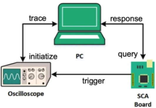
The overall measurement setup is depicted in Figure 2. The microcontroller is clocked at 16M Hz and runs the AES-128 algorithm in software. The board is connected to a two-channel Tektronix TDS2012 oscilloscope with a sampling rate of 2GS/s (Giga-samples per second). The power traces are captured corresponding to AES-128 execution, synchronized with a board generated trigger. A computer is used to pilot

Fig. 2: Illustration of the measurement setup.

the whole setup. It generates random 128-bit plaintext and, via UART, transmits it to the board and awaits acknowledgment of the ciphertext. Upon receiving ciphertext, the software then retrieves the waveform samples from an oscilloscope and saves it to hard-drive indexed with corresponding plaintext and ciphertext. To minimize the storage overhead, the trace comprised of 600 sample points (features) captures only the execution of the first SubBytes call, i.e., the target of the following attacks (the output of the first AES S-box in the SubBytes layer). The AES S-box is an 8-bit input to an 8-bit output mapping, which computes multiplicative inverse fol-lowed by an affine transformation on polynomials over GF (2). For performance reasons, it is implemented as a precomputed look-up table. The table is indexed with p[0] ⊕ k[0], where (p[0], k[0]) are the first bytes of plaintext and key, respectively. The output of the S-box is stored in the internal registers or memory of the microcontroller and is the main side-channel leakage that we target. The labeling of data is done on the output byte of the box. Due to the nonlinearity of the S-box, it is much easier to statistically distinguish the correct key from wrong keys at the output of the S-box, which is why we choose to attack here.

Figure 3 shows an example measurement trace for the full amount of 600 features on the top. Below is the correlation between the measurement set and the activity corresponding to the S-box look-up with the first byte of plaintext. We highlight the 50 features with the highest absolute Pearson correlation in red. One can see that these 50 features cover nearly all leaking points.

Finally, in order to investigate the influence of the number of training examples, we consider settings with 10 000 and 40 000 measurements in the training phase. In total, we conducted more than 150 experiments in order to provide a detailed analysis of the subject.

C. Parallel Measurement

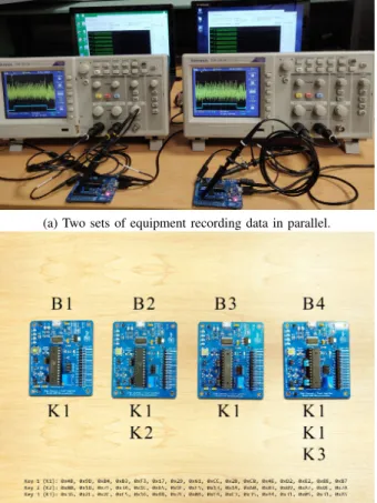
We use four copies of the target device to conduct our study. Four experiments were set up in parallel (two parallel setups shown in Figure 4a). Parallel setups allowed us to collect the experimental data faster as well as to minimize the effect of change in environmental conditions. To be able to test different scenarios, we measured 50 000 side-channel leakage

measure-Fig. 3: Measurement trace and corresponding correlation (se-lected 50 features in red).

ments corresponding to 50 000 random plaintext on different boards (B1, B2, B3, B4) with three randomly chosen secret keys. In the following, each dataset is denoted in the format Bx Ky, where x denotes board ID and y denotes the key ID. For example, B1 K1, denotes the dataset corresponding to K1 measured on board B1. The four boards and keys used for collecting various datasets are shown in Figure 4b. In this case, B4 K1 is repeated. This provides a benchmark comparison in the scenario where both the device and the keys are the same, although not measured at the same time.

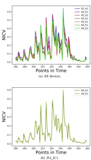
Although the measurement setups are identical, executing exactly the same code and measuring the same operations, there will still be some difference due to process and envi-ronmental factors. To highlight the difference of the leakages from different devices, we calculate Normalized Inter-Class Variance (NICV [24]). NICV can be used to detect relevant leakage points in side-channel traces as well as to compare the quality of side-channel measurements. It is computed as:

N ICV = V{E{T |X}} V{T }

, (1) where T denotes a side-channel trace and X is the public parameter (plaintext/ciphertext), used to partition the traces. E{·} and V{·} are statistical expectation and variance. NICV is bounded in the range [0, 1].

From Figure 5a, it is clear that even for similar im-plementations, the leakage differs, and each setting has its leakage characteristics. The impact of these differences will be evaluated in the following sections using machine learning-based profiled side-channel attacks. As a comparison, for the same device and key scenario (B4 K1), as given in Figure 5b, the NICV pattern is almost completely the same.

D. Scenarios under Consideration

In our experiments, we consider several scenarios with respect to the targets:

• Same device and same key. In this setting, we use the same device and only a single key to conduct both profiling/validation and attack. Despite the fact that this scenario is far from the realistic setting, it is usually explored in the SCA community. Consequently, most of the works consider this scenario and report results for it.

(a) Two sets of equipment recording data in parallel.

(b) SCA Boards labelled with different keys.

Fig. 4: Parallel equipment setup. The three keys are randomly generated. The keys are repeated across different boards to test the impact of varying target board and the secret key in various configurations.

We emphasize that this is also the simplest scenario for the attacker.

• Same device and different key. In this scenario, we assume there is only one device to conduct both profiling and attack, but the key is different in those two phases. This scenario can sound unrealistic since there is only one device, but we still consider it as an interesting stepping stone toward more realistic (but also more difficult) scenarios.

• Different device and same key. Here, we assume there

are two devices (one for profiling and the second one for the attack) that use the same key. While this scenario can again sound unrealistic, we note that it emulates the setting where one key would be hardcoded on a number of devices.

• Different device and different key. This represents the

realistic setting since it assumes one device to train and a second device to attack. Additionally, the keys are different on those devices.

To the best of our knowledge, such a variety of considered scenarios have never been investigated before.

280 290 300 310 320 330 340 350 360

Points in Time

NICV

(a) All devices.

280 290 300 310 320 330 340 350 360

Points in Time

NICV

Fig. 5: NICV comparison.

E. Hyper-parameter Tuning

In our experiments, we consider the following machine learning techniques: NB, RF, MLP, and CNN. We select these four techniques as they are well-investigated in the SCA community and known to give good results [31], [12], [23], [19], [13]. NB is an often considered technique in SCA as it is very simple and has no hyper-parameters to tune. Additionally, it shows good performance when the data is limited [31]. RF shows very good performance in SCA and is often considered as the best-performing algorithm (when not considering deep learning) [16], [18]. From deep learning techniques, CNN performs well when there is random delay countermeasure due to its spatial invariance property [13], [23]. Finally, an MLP works well for masking countermeasures as it combines all features and produces the effect of a higher-order attack [13], [19].

We also distinguish between two settings for these tech-niques:

• In the first setting, we select 50 most important features to run the experiments. To select those features, we use the Pearson correlation. The Pearson correlation coefficient

measures linear dependence between two variables, x and y, in the range [−1, 1], where 1 is the total positive linear correlation, 0 is no linear correlation, and −1 is the total negative linear correlation. Pearson correlation for a sample of the entire population is defined by [32]:

P earson(x, y) =

PN

i=1((xi− ¯x)(yi− ¯y))

q PN i=1(xi− ¯x)2 q PN i=1(yi− ¯y)2 . (2) We note that the Pearson correlation is a standard way for feature selection in the profiled SCA, see, e.g., [33], [34]. Additionally, Picek et al. show that while it is not the best feature selection in all scenarios, Pearson correlation behaves well over a number of different profiled SCA settings [35]. In this setting, we use NB, RF, and MLP.

• In the second setting, we consider the full set of features (i.e., all 600 features) and we conduct experiments with MLP and CNN. Note that MLP is used in both scenarios since it can work with a large number of features but also does not need the features in the raw form (like CNN). For the experiments with 50 features, we use scikit-learn [36], while for the experiments with all features, we use Keras [37]. For NB, RF, and MLP when using 50 features, we use k-fold cross-validation with k = 5. For experiments when using all features, we use three datasets: train, validate, and test. Training set sizes are 10 000 and 40 000, validation set size equals 3 000, and test set size equals 10 000. Since there is in total 50 000 measurements with 10 000 measurements used for testing, when using the validation set, then the largest training set size is not 40 000 but 37 000.

a) Naive Bayes: NB has no parameters to tune.

b) Random Forest: For RF, we experimented with the number of trees in the range [10, 100, 200, 300, 400]. Based on the results, we use 400 trees with no limit to the tree depth.

c) Multilayer Perceptron: When considering scenarios with 50 features, we investigate [relu, tanh] activation func-tions and the following number of hidden layers [1, 2, 3, 4, 5] and a number of neurons [10, 20, 25, 30, 40, 50].

Based on our tuning phase, we selected (50, 25, 50) ar-chitecture with relu activation function (recall, ReLU is of the form max(0, x)). We use the adam optimizer, the initial learning rate of 0.001, log − loss function, and a batch size of 200.

When considering all features and MLP, we investigate the following number of hidden layers [1, 2, 3, 4] and number of neurons [100, 200, 300, 400, 500, 600, 700, 800, 900, 1 000]. Based on the results, we select to use four hidden layers where each layer has 500 neurons. We set the batch size to 256, the number of epochs to 50, the loss function is categorical cross-entropy, and optimizer is RM Sprop with a learning rate of 0.001.

d) Convolutional Neural Network: For CNN, we con-sider architectures of up to five convolutional blocks and two fully-connected layers. Each block consists of a convolutional layer with relu activation function and average pooling layer. The first convolutional layer has a filter size of 64 and then

each next layer increases the filter size by a factor of 2. The maximal filter size is 512 and the kernel size is 11. For the average pooling layer, pooling size is 2 and stride is 2. Fully-connected layers have relu activation function and we experiment with [128, 256, 512] number of neurons. After a tuning phase, we select to use a single convolutional block and two fully-connected layers with 128 neurons each. Batch size equals 256, the number of epochs is 125, the loss function is categorical cross-entropy, the learning rate is 0.0001, and the optimizer is RM Sprop.

IV. RESULTS

In this section, we present results for all scenarios we investigate. Afterward, we discuss the issues with the val-idation procedure and present our Multiple Device Model. As mentioned earlier, we use guessing entropy as the metric for comparison. In other words, we observe the average rank of the key against the number of traces or measurement samples. An attack is effective if the guessing entropy goes to 0 with minimum required samples. If at the end of attack guessing entropy stays at x, the attacker must brute force 2x different keys for key recovery. Note that we give averaged results for a certain machine learning technique and number of measurements. We denote the scenario where we use a multilayer perceptron with all 600 features as MLP2, while the scenario where multilayer perceptron uses 50 features we denote as MLP.

A. Same Key and Same Device

The first scenario we consider uses the same devices and keys for both training and testing phases. Consequently, this scenario is not a realistic one but is a common sce-nario examined in the related works. This scesce-nario does not consider any portability aspect and is the simplest one for machine learning techniques, so we consider it as the baseline case. The results for all considered machine learning techniques are given in Figure 6. We give averaged results over the following settings: (B1 K1)−(B1 K1), (B2 K2)− B2 K2), (B3 K1) − (B3 K1), (B4 K3) − (B4 K3). As can be seen, all results are very good, and even the worst-performing algorithm reaches guessing entropy of 0 in less than 10 measurements. Thus, an attacker would need only 10 side-channel traces from the target device to perform the full key-recovery. Additionally, we see that adding more measurements can improve the performance of attacks. The worst performing algorithm is NB, followed by RF. The differences among other algorithms are very small and we see that guessing entropy reaches 0 after three measurements. Note that despite somewhat smaller training sets (37 000) for algorithms using all 600 features (CNN and MLP2), those results do not show any performance deterioration. In fact, the algorithms can reach guessing entropy of 0 with up to three traces. Since we are using the same device and key to train and attack, and we are using validation or cross-validation to prevent overfitting, accuracy in the training phase is only

Fig. 6: Same device and key scenario.

Fig. 7: Same device and different key scenario.

somewhat higher than accuracy in the test phase (depending on the algorithm, ≈ 10 − 40%).

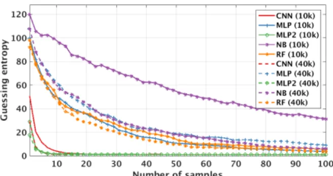
B. Same Device and Different Key

Next, we consider the scenario where we use the same device in the training phase and testing phase, but we change keys between those phases. When different users compute on shared resources and standard cryptographic libraries (like SSL), this scenario becomes relevant. The malicious user profiles the library with his application with all access rights and attacks when the target user application is running. We present the results for this scenario in Figure 7. Here, we give averaged results over scenarios (B2 K1)−(B2 K2) and (B2 K2) − (B2 K1). The first observation is that this setting is more difficult for machine learning algorithms. Indeed, NB, RF, and MLP (using 50 features) require more than 100 measurements to reach guessing entropy less than 10 (note that NB with 10 000 measurements reaches only guessing entropy of around 40). Interestingly, for these three techniques, adding more measurements (i.e., going from 10 000 to 40 000) does not bring a significant improvement in performance. At the same time, both techniques working with all features (MLP2 and CNN) do not seem to experience performance degradation when compared to the first scenario. Regardless of the number of measurements in the training phase, they reach guessing entropy of 0 after three measurements. For this scenario, we observed that accuracy in the training phase could be up to an order of magnitude better than accuracy in the test phase, which indicates that our algorithms overfit.

Fig. 8: Same key and different device scenario.

C. Same Key and Different Device

The third scenario we consider uses two different devices, but the key stays the same. Note, since we consider dif-ferent devices, we can talk about the real-world case, but the same key makes it still a highly unlikely scenario. The results are averaged over settings (B1 K1) − (B2 K1) and (B2 K1)−(B1 K1). When considering performance, we see in Figure 8 that this scenario is more difficult than the previous two as different targets introduce their noise patterns. Similar to the previous scenario, all techniques using 50 features require more than 100 measurements to reach guessing entropy less than 10. Additionally, adding more measurements does not improve results significantly. When considering techniques using all 600 features, we see this scenario to be more difficult than the previous ones as we need seven or more traces to reach guessing entropy of 0. Additionally, CNN using 10 000 measurements is clearly performing worse than when using 40 000 measurements, which is a clear indicator that we require more measurements to avoid underfitting on the training data. Finally, we remark that in these experiments, accuracy in the training set was up to an order of magnitude higher than for the test set. Consequently, we see that while we require more measurements in the training phase to reach the full model capacity, those models already overfit as the differences between devices are too significant.

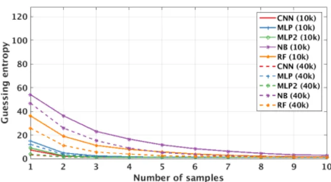
D. Different Key and Device

Finally, we investigate the setting where training and testing are done on different devices and those devices use different secret keys. Consequently, this is the full portability scenario one would encounter in practice. As expected, this is by far the most difficult scenario for all techniques, as seen in Figure 9. In this scenario, the results are averaged over 8 dif-ferent settings: (B1 K1) − (B4 K3), (B4 K3) − (B1 K1), (B2 K2) − (B4 K3), (B4 K3) − (B2 K2), (B3 K1) − (B4 K3), (B4 K3) − (B3 K1), (B1 K1) − (B2 K2), and (B2 K2) − (B1 K1).

Interestingly, here RF is the worst performing algorithm, and with 100 measurements, it barely manages to reach guessing entropy less than 90. NB and MLP perform better, but still with 100 measurements, they are not able to reach guessing entropy less than 15. At the same time, we see

Fig. 9: Different key and device scenario.

a clear benefit of added measurements only for NB. When considering CNN and MLP2, we observe we require somewhat more than 60 measurements to reach guessing entropy of 0. There is a significant difference in performance for CNN when comparing settings with 10 000 and 40 000 measurements. For MLP2, that difference is much smaller and when having a smaller number of measurements, MLP2 outperforms CNN.

When CNN uses 40 000 measurements in the training phase, it outperforms MLP2 with 10 000 measurements and both techniques reach guessing entropy of 0 with the approximately same number of measurements in the testing phase. As in the previous scenario, we see that CNN needs more measurements to build a strong model. This is in accordance with the intuitive difficulty of the problem as more difficult problems need more data to avoid underfitting and to reach good model complexity. Interestingly, in this scenario, accuracy for the training set is easily two orders of magnitude higher than for the test set, which shows that all techniques overfit significantly. Indeed, while we see that we can build even stronger models if we use more measurements in the training phase, such obtained models are too specialized for the training data and do not generalize well for the test data obtained from different devices.

E. General Observations

When considering machine learning techniques we used and investigated scenarios, we see that MLP2 performs the best (the difference with CNN is small, especially if considering 40 000 measurements in the training phase). In order to better understand the difficulties stemming from specific scenarios, we depict the result for MLP2 and all four scenarios in Figure 10.

Clearly, the first two scenarios (having the same device and key as well as changing the key but keeping the same device) are the easiest. Here, we see that the results for the scenario when changing the key indicate it is even slightly easier than the scenario with the same device and key. While other machine learning techniques point that using the same key and device is the easiest scenario, they all show these two scenarios to be easy. Next, a somewhat more difficult case is the scenario where we change the device and use the same key. Again, the exact level of increased difficulty depends on the

Fig. 10: Multilayer perceptron with 600 features (MLP2) over all scenarios, 10 000 measurements.

specific machine learning algorithm. Finally, the most difficult scenario is when we use different devices and keys. Here, we can see that the effect of portability is much larger than the sum of previously considered effects (changing only key or device).

While all scenarios must be considered as relatively easy when looking at the number of traces needed to reach guessing entropy of 0, the increase in the number of required measure-ments is highly indicative of how difficult problem portability represents. Indeed, it is easy to see that we require more than an order of magnitude more measurements for the same performance if we consider scenarios three and four. At the same time, already for scenario three, we require double the measurements than for scenarios one or two.

While we use only a limited number of experimental settings, there are several general observations we can make: 1) Any portability setting adds to the difficulty of the

problem for machine learning.

2) Attacking different devices is more difficult than attacking different keys.

3) The combined effect of different key and different device is much larger than their sum.

4) Adding more measurements does not necessarily help but, on average, also does not deteriorate the performance. 5) CNN requires more measurements in portability settings

to build strong models.

6) While our results indicate that additional measurements in the training phase would be beneficial to reach the full model capacity, we observe that in portability settings, there is a significant amount of overfitting. This represents an interesting situation where we simultaneously underfit on training data and overfit on testing data.

7) The overfitting occurs because we do not train on the same data distribution as we test.

V. MULTIPLEDEVICEMODEL

In this section, we first discuss the overfitting issue we encounter in portability. Next, we propose a new model for portability called the Multiple Device Model, where we experimentally show its superiority when compared to the usual setting.

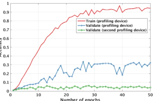
Fig. 11: Training and validation on the same device vs. validation done on different device.

A. Overfitting

Recall from Section II-B1 that we are interested in super-vised learning where, based on training examples (data X and corresponding labels Y ), a function f is obtained. That function is later used on testing data to predict the corre-sponding labels. Here, the function f is estimated from the observed data. That observed data is drawn independently and identically distributed from a common distribution. To avoid overfitting, we use validation (e.g., k-fold cross-validation or a separate dataset for validation).

As it can be observed from the results in the previous section, when training and testing data come from the same device, the machine learning techniques do not have problems in building good models as the model is fitted to the same distribution of data as will be used in the attack phase. There, validation on the same data distribution helps to prevent overfitting.

However, when there are two devices, one for training and the second one to attack, the problem of overfitting is much more pronounced and having validation done on a training de-vice does not help significantly. Naturally, the problem is that our model is fitted to the training data, but we aim to predict testing data, which may not have the same distributions. We depict this in Figure 11, where we show results for training and validation on the device B1 K1 versus training on the device B1 K1 and validation on the device B4 K3. In this scenario, we experiment with MLP2 and we use all features. We can clearly observe that when conducting validation on the same device as training, the accuracy increases with the number of epochs. At the same time, when we run validation with measurements from a different device, there is almost no improvement coming from a longer training process.

Based on these results, we identify overfitting as one of the main problems in the portability scenarios. There, overfitting occurs much sooner than indicated by validation if done on the same device as training. Additionally, our experiments indicate that k-fold cross-validation suffers more from portability than having a separate validation dataset. This is because it allows

a more fine-grained tuning, which further eases overfitting. To prevent overfitting, there are several intuitive options: 1) Adding more measurements. While this sounds like a

good option, it can bring some issues as we cannot know how much data needs to be added (generally in SCA, we will, already, use all the available data from the start). Also, in SCA, a longer measurement setup may introduce additional artifacts in the data distribution [38]. Finally, simply increasing the amount of training data does not guarantee to prevent overfitting as we do not know what amount of data one needs to prevent underfitting. 2) Restricting model complexity. If we use a model that has

too much capacity, we can reduce it by changing the network parameters or structure. Our experiments also show the benefits of using more shallow networks or shorter tuning phases, but it is difficult to estimate a proper setting without observing the data coming from the other distribution.

3) Regularization. There are multiple options here: dropout, adding noise to the training data, activation regulariza-tion, etc. While these options would certainly reduce overfitting in general case, they are unable to assess when overfitting actually starts for data coming from a different device, which makes them less appropriate for the portability scenarios. We note that some of these techniques have also been used in profiled SCA but not in portability settings, see, e.g., [13], [23].

B. New Model

Validation on the same device as training can seriously affect the performance of machine learning algorithms if attacking a different device. Consequently, we propose a new model that uses multiple devices for training and validation. We emphasize that since portability is more pronounced when considering different devices than different keys (and their combined effect is much larger than their sum), it is not sufficient to build the training set by just using multiple keys and one device. Indeed, this is a usual procedure done for template attack, but it is insufficient for full portability considerations.

In its simplest form, our new model, called the “Multiple Device Model” (abbreviated MDM) consists of three devices: two for training and validation and one for testing. Since we use more than one device for training and validation, the question is which device to use for train and which one for validation. The simplest setting is to use one device for training and the second one for validation. In that way, we can prevent overfitting as the model will not be able to learn the training data too well. Still, there are some issues with this approach: while we said we use one device for training and the second one for validation, it is still not clear how to select which device to use for what. Indeed, our results clearly show that training on device x and validating on device y to attack device z will produce different results when compared to training on device y and validating on device x to attack device z. This

happens because we cannot know whether device x or y is more similar to device z, which will influence the final results. Instead of deciding on how to divide devices among phases, we propose the Multiple Device Model where a number of devices participate in training and validation. More formally, let the attacker has on his disposal t devices with N data pairs xi, yifrom each device. The attacker then takes the same

number of measurements k from each device to create a new train set and the same number of measurements j from each device to create a validation set. Naturally, the measurements in the training and validation sets need to be different. The training set then has the size t·k and the validation set has size t · j. With those measurements, the attacker builds a model f , which is then used to predict labels for measurements obtained from a device under attack. We emphasize that in training and validation, it is necessary to maintain a balanced composition of measurements from all available devices in order not to build a model skewed toward a certain device. We depict the MDM setting in Figure 12.

Definition 2: Multiple Device Model denotes all settings where attacker can conduct the training on measurement data from a number of similar devices (≥ 2), −→B = { ˆB0,...,

ˆ

Bn−1} and import the learned knowledge L−→_B to model the

actual device under target B, under similar but uncontrolled parameter setup P .

We present results for MDM and multilayer perceptron that uses all features (MLP2) and 10 000 measurements as it provided the best results in the previous section. The results are for specific scenarios, so they slightly differ from previous results where we depict averaged results over all device combinations. Finally, we consider here only the scenario where training and attacking are done on different devices and use different keys. Consequently, the investigated settings are selected so as not to allow the same key or device to be used in the training/validation/attack phases.

In Figure 13a, we depict several experiments when us-ing different devices for trainus-ing and validation. First, let us consider the cases (B1 K1) − (B4 K3) − (B2 K2) and (B1 K1) − (B2 K2). There, having separate devices for training and validation improves over the case where validation is done on the same device as training. On the other hand, cases (B4 K3) − (B2 K2) − (B1 K1) and (B4 K3) − (B1 K1) as well as (B4 K3) − (B1 K1) − (B2 K2) and (B4 K3) − (B2 K2) show that adding de-vice for validation actually significantly degrades the per-formance. This happens because the difference between the training and validation device is larger than the difference between the training and testing device. Next, the cases (B2 K2) − (B4 K3) − (B1 K1) and (B2 K2) − (B1 K1) show very similar behavior, which means that validation and testing datasets have similar distributions. Finally, for three devices, e.g., cases (B1 K1) − (B4 K3) − (B2 K2) and (B4 K3) − (B1 K1) − (B2 K2), the only difference is the choice of training and validation device/key. Nevertheless, the performance difference is tremendous, which clearly shows the limitations one could expect if having separate devices for

Device1

Labels

Classification

Algorithm

Device

Tracestest

Label

Classification

Algorithm

Secret

Key

Profiled

Model

Profiling Phase Attack Phase

Tracesval

Device2

Device3

Fig. 12: Illustration of the proposed MDM. Observe a clear separation between training/validation devices and a device under attack, cf. Figure 1.

training and validation.

Next, in Figure 13b, we depict the results for our new Multiple Device Model where training and validation mea-surements come from two devices (denoted with “multiple” in the legend). As it can be clearly seen, our model can improve the performance significantly for two out of three experiments. There, we can reach the level of performance as for the same key and device scenario. For the third experiment, (B1 K1) − (B2 K2) − (B4 K3), we see that the improvement is smaller but still noticeable, especially for certain ranges of the number of measurements. We see that MDM can result in order of magnitude better performance than using two devices. At the same time, with MDM, we did not observe any case where it would result in performance degradation when compared to the usual setting.

In summary, we show that MDM offers a superior model by clearly establishing different sets of devices for training, validation, and attack. The improvements obtained, compared to the usual setting of two devices, measured in terms of guessing entropy is > 10× (i.e., two traces with the MDM model, while over 20 traces with two devices). The perfor-mance impact of various scenarios is studied systematically to highlight the pitfalls clearly. MDM may not always be necessary: if both training and attacking devices contain small levels of noise and are sufficiently similar, then using only those two devices could suffice. Still, as realistic settings tend to be much more difficult to attack, having multiple devices for training and validation would benefit attack performance significantly. While MDM requires a strong assumption on the attacker’s capability (i.e., to have multiple devices of the same type as the device under attack), we consider it to be well within realistic scenarios. If additional devices are not available, one could simulate it by adding a certain level of noise to the measurements from the training device.

VI. OVERCOMING THEHUMANERROR: PORTABILITY OF

ELECTROMAGNETICPROBEPLACEMENT

Electromagnetic measurements are very sensitive to probe placement (position, distance, and orientation). This does not

(a) Results for separate devices for training and validation.

(b) Results for MDM.

Fig. 13: Results for different settings with multiple devices for training and validation.

represent a problem in “classical” side-channel measurements where training and testing are done on the same device as the probe does not move. However, if we consider the realistic profiled scenario, training and testing must be done on different devices. This essentially means the probe must be moved from training to the testing device. Even though

the placement of the probe on the testing device can be very close to that on the training device, there is always a small difference in the placement due to the position distance and orientation. We attribute this error of placement as the human error.

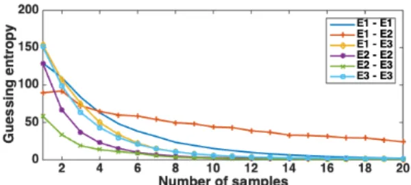
To investigate the impact of human error, we performed the following experiment. Measurements are taken of an Ar-duino Uno board, fitted with previously investigated AVR AT-MEGA328P, running AES-128 encryption. The measurements are taken around a target S-box computation in the first round (one byte), with Lecroy WaveRunner 610zi oscilloscope using an RF-U 5-2 near-field EM probe from Langer and amplified by a 30 dB pre-amplifier. Three datasets (E1, E2, E3) are captured for random plaintext, each time at a similar position but with the aforementioned human error. The datasets have 50 000 traces where each trace has 500 features. We use a MLP and we first conduct a tuning phase with the same hyper-parameters as before. We again use the same setting with 10 000 traces in the testing phase and 10 000 or 40 000 traces in the training phase. The validation set has 3 000 traces.

Based on that tuning phase, we decide to use an MLP with two hidden layers where each hidden layer has 100 neurons. We depict the results in Figure 14. We can observe that MDM helps us to 1) obtain better results, i.e., reach guessing entropy equal to 0 faster, and 2) make the performance more stable across device combinations. Again, we can observe that having a smaller number of traces for training does not necessarily mean the performance of the attack will be decreased. This is especially clear in Figure 14c, where most of the cases do not reach guessing entropy of 0 within 20 attack traces. This is contrasting Figure 14a, where we observe only one such case and, of course, Figures 14b and 14d, where MDM ensures significantly better attack performance.

VII. RELATEDWORK ONPORTABILITY

The problem of portability stems from the issue of overfit-ting, which is a common issue in machine learning. Exploring portability in the context of profiled SCA received only limited attention up to now. Elaabid and Guilley highlighted certain issues with template attacks, such as when the setups changed, for example, due to desynchronization or amplitude change [39]. They proposed two pre-processing methods to handle the templates mismatches: waveform realignment and acquisition campaigns normalization. Choudary and Kuhn analyzed profiled attacks on four different Atmel XMEGA 256 8-bit devices [40]. They showed that even on similar devices, the differences could be observed that make the attack harder and carefully tailored template attacks could help to mitigate the portability issue. Device variability was also a consideration in hardware Trojan detection [9]. There, the authors showed that the results are highly biased by the process variation. The experiments were conducted on a set of 10 Virtex-5 FPGAs. Kim et al. demonstrated the portability in the case of wireless keyboard, by building the template based on the recovered AES key to attack another keyboard [11]. They highlighted that some correction has to be performed

(a) Classical approach and different EM probes positions, 10 000 measurements.

(b) MDM approach for different positions of EM probes, 10 000 measurements.

(c) Classical approach and different EM probes positions, 40 000 measurements.

(d) MDM approach for different positions of EM probes, 40 000 measurements.

Fig. 14: Portability of Electromagnetic Probe Placement.

before directly using the built templates. In 2018, the CHES conference announced a side-channel CTF event for “Deep learning vs. classic profiling”, which also considers the case of portability. One of the contest categories was protected AES implementation. The winning attack was a combination of a linear classifier (decision tree and perceptron) and SAT solver. The attack needed five traces and 44 hours of SAT solver time to achieve 100% success for different devices, but only one trace was enough for attacking the same device [41]. To summarize, all previous works applied a target specific pre-processing or post-pre-processing to fight portability.

Very recently, two studies have been reported with a focus on portability. A cross-device side-channel attack was

pre-sented in [42], where the authors aim to propose a neural network architecture optimized for the cross-device attack, and in the process, highlight the problem of portability. Recently, Carbone et al. used deep learning to attack an RSA implementation on an EAL4+ certified target [43]. In both the works, the authors used several devices for various stages of a profiled attack (i.e., training/validation/attack). The classification algorithm (MLP/CNN in their case) was trained with traces from two devices and tested on a third device. Interestingly, their observations agree with our results that deep learning can help overcome portability when trained with multiple devices. However, their focus lies in demonstrating the feasibility of the attack in the presence of portability. In contrast, we study the core problem of portability, identify the limitations of state-of-the-art techniques through extensive practical experiments, and propose a methodology based on MDM. We believe that this work will pave the way for realistic studies on SCA.

VIII. CONCLUSIONS ANDFUTUREWORK

In this paper, we tackle the portability issue in machine learning-based side-channel attacks. We show how even small differences between devices can cause attacks to perform significantly differently. As expected, our results clearly show that the scenario where we use different keys and devices in the profiling and attacking phase is the most difficult one. This is important because it means that most of the attacks conducted in related works greatly overestimate their power as they use the same device and key for both training and attack. We identify the validation procedure as one of the pitfalls for portability and machine learning. Consequently, we propose Multiple Device Modelto report > 10× improvement in attack performance.

In our experiments, we considered homogeneous platforms with no countermeasures. The choice was motivated by finding the best case measurements to focus on portability problems. In future work, we plan to extend this approach to hetero-geneous platforms. It would also be interesting to investigate what is the influence of various countermeasures (both hiding and masking) to the performance of machine learning clas-sifiers when considering portability. Additionally, we plan to experiment with a larger number of devices to improve the generalization capabilities of machine learning algorithms.

Moreover, it is not always possible to assume the availability of multiple devices to perform training under the Multiple Device Model. In such settings, the adversary would need to resort to simulation. Ideally, it is straightforward to simulate multiple devices (or components) by running Monte Carlo simulations with available process variation models, which is widely popular in VLSI design. This simulation method-ology can simply be extended to the board level, which is a combination of several distinct devices with individual process variation models. Note that the viability and accuracy of this simulation methodology entirely depend on the availability and precision of the process variation model, which are proprietary to the manufacturer and might not be easily available. Practical

evaluation of the robustness of MDM with this simulation methodology will be an interesting extension of this work. Finally, our experiments indicate that smaller datasets could be less prone to overfitting. It would be interesting to see whether we can obtain good performance with small training set sizes, which would conform to setting as described in [44].

ACKNOWLEDGMENT

This research is partly supported by the Singapore National Research Foundation under its National Cybersecurity R&D Grant (“Cyber-Hardware Forensics & Assurance Evaluation R&D Programme” grant NRF2018–NCR–NCR009–0001).

REFERENCES

[1] P. C. Kocher, “Timing attacks on implementations of diffie-hellman, rsa, dss, and other systems,” in Advances in Cryptology - CRYPTO ’96, 16th Annual International Cryptology Conference, Santa Barbara, California, USA, August 18-22, 1996, Proceedings, ser. Lecture Notes in Computer Science, N. Koblitz, Ed., vol. 1109. Springer, 1996, pp. 104–113. [Online]. Available: http://dx.doi.org/10.1007/3-540-68697-5 9 [2] ——, “Timing Attacks on Implementations of Diffie-Hellman, RSA,

DSS, and Other Systems,” in Proceedings of CRYPTO’96, ser. LNCS, vol. 1109. Springer-Verlag, 1996, pp. 104–113.

[3] P. C. Kocher, J. Jaffe, and B. Jun, “Differential power analysis,” in Proceedings of the 19th Annual International Cryptology Conference on Advances in Cryptology, ser. CRYPTO ’99. London, UK, UK: Springer-Verlag, 1999, pp. 388–397. [Online]. Available: http: //dl.acm.org/citation.cfm?id=646764.703989

[4] J.-J. Quisquater and D. Samyde, “Electromagnetic analysis (ema): Mea-sures and counter-meaMea-sures for smart cards,” in Smart Card Program-ming and Security, I. Attali and T. Jensen, Eds. Berlin, Heidelberg: Springer Berlin Heidelberg, 2001, pp. 200–210.

[5] M. Lipp, M. Schwarz, D. Gruss, T. Prescher, W. Haas, A. Fogh, J. Horn, S. Mangard, P. Kocher, D. Genkin, Y. Yarom, and M. Hamburg, “Meltdown: Reading kernel memory from user space,” in 27th USENIX Security Symposium (USENIX Security 18), 2018.

[6] M. Zhao and G. E. Suh, “Fpga-based remote power side-channel attacks,” in 2018 IEEE Symposium on Security and Privacy (SP). IEEE, 2018, pp. 229–244.

[7] S. Chari, J. R. Rao, and P. Rohatgi, “Template Attacks,” in CHES, ser. LNCS, vol. 2523. Springer, August 2002, pp. 13–28, San Francisco Bay (Redwood City), USA.

[8] O. Choudary and M. G. Kuhn, “Efficient template attacks,” in Interna-tional Conference on Smart Card Research and Advanced Applications. Springer, 2013, pp. 253–270.

[9] X. T. Ngo, Z. Najm, S. Bhasin, S. Guilley, and J.-L. Danger, “Method taking into account process dispersion to detect hardware trojan horse by side-channel analysis,” Journal of Cryptographic Engineering, vol. 6, no. 3, pp. 239–247, 2016.

[10] M. Renauld, F.-X. Standaert, N. Veyrat-Charvillon, D. Kamel, and D. Flandre, “A formal study of power variability issues and side-channel attacks for nanoscale devices,” in Annual International Conference on the Theory and Applications of Cryptographic Techniques. Springer, 2011, pp. 109–128.

[11] K. Kim, T. H. Kim, T. Kim, and S. Ryu, “Aes wireless keyboard: Template attack for eavesdropping,” Black Hat Asia, Singapore, 2018. [12] H. Maghrebi, T. Portigliatti, and E. Prouff, “Breaking cryptographic

implementations using deep learning techniques,” in Security, Privacy, and Applied Cryptography Engineering - 6th International Conference, SPACE 2016, Hyderabad, India, December 14-18, 2016, Proceedings, 2016, pp. 3–26.

[13] E. Cagli, C. Dumas, and E. Prouff, “Convolutional Neural Networks with Data Augmentation Against Jitter-Based Countermeasures - Profil-ing Attacks Without Pre-processProfil-ing,” in Cryptographic Hardware and Embedded Systems - CHES 2017 - 19th International Conference, Taipei, Taiwan, September 25-28, 2017, Proceedings, 2017, pp. 45–68.