Automatic 3D localisation system using propagation of positions in a connected network

(1)

HAL Id: hal-01366513

https://hal.archives-ouvertes.fr/hal-01366513

Submitted on 14 Sep 2016

HAL is a multi-disciplinary open access archive for the deposit and dissemination of sci-entific research documents, whether they are pub-lished or not. The documents may come from teaching and research institutions in France or abroad, or from public or private research centers.

L’archive ouverte pluridisciplinaire HAL, est destinée au dépôt et à la diffusion de documents scientifiques de niveau recherche, publiés ou non, émanant des établissements d’enseignement et de recherche français ou étrangers, des laboratoires publics ou privés.

Automatic 3D localisation system using propagation of

positions in a connected network

Magda Chelly, Nel Samama

To cite this version:

Magda Chelly, Nel Samama. Automatic 3D localisation system using propagation of positions in a connected network. ENC-GNSS 2009 : European Navigation Conference - Global Navigation Satellite Systems, May 2009, Naples, Italy. �hal-01366513�

(2)

Automatic 3D Localisation System Using

Propagation of Positions in a Connected Network

Magda Chelly, Institut TELECOM / T&M SudParis. Samama Nel, Institut TELECOM / T&M SudParis.

BIOGRAPHY

Magda Chelly received his engineering diploma in Telecommunications in 2007, and a Masters degree in the Architecture of Telecommunication Systems in 2008, both from the “Ecole Supérieure des Télécommunications de Tunis”, Tunisia. She’s a Ph.D. student in Telecommunications in the “TELECOM & Management SudParis”, Evry, France. She’s working on indoor positioning systems.

Nel Samama is member of the Navigation Group at IT-SudParis. He has been working for many years in the GPS field, on projects such as the development of new communication schemes and indoor location techniques. Its current interest is to find a simple approach for a standard GPS receiver to enable indoor positioning.

INTRODUCTION

Nowadays, environment can contain various telecommunication networks. These (local or wide) area networks are composed by mobile or static points, connected or not, called nodes of the network. They can constitute the key of a graphic or diagrammatic modeling of the environment. The objective of this part of work is to model any environment outdoor or indoor using the nodes of the networks and the relations between them. So it will be supposed that among the nodes constituting these networks, there are some which have known geographical positions and others which have not, in an absolute referential. The approach is based on the spatial

relations between these nodes in order to build a two-dimensional or three-dimensional graph representing the distribution of the nodes in the environment. To express these relations, we take to consideration two approaches. The first one is based on an algebraic method in order to elaborate the model of the environment and the second one is based on the theory of spatial reasoning. Our work is divided in two parts. Models obtained are compared and tested in order to evaluate their performance.

I. ALGEBRAIC APPROACH

We consider an environment with a certain number of networks for which we don’t have information about the size, the topology. These networks are made of different nodes. The nodes are distributed outdoors and indoors. The outdoor nodes can eventually have their geographical coordinates. The other nodes have not yet any positioning information. We describe here an approach involving the algebraic calculation in order to model our environment [1] [2].

I.1 THEORETICAL BASES

The first step consists of having an idea about the global notions used below. A graph is defined as a structure to model the relationships between elements of a collection. A graph consists in vertices connected by arcs (if the connection is unidirectional) and bones (if the connection is bidirectional). The graphs generalize the concept of binary relations. However, in our work, we extend the research to other cases. We modify the concept on which is

(3)

based a graph. The principle consists to find exactly one path from one node to another. Nodes could be connected or not connected. A probabilistic approach allow to estimate that for a graph with n nodes and m arcs, each pair of nodes can be related with a probability p. If p equals zero, there is no connection between nodes and if it equals 1 there is a connection. In a graph, each node and each edge are labeled. The labeling of a graph can be designed, for example, to provide useful information for routing problems. The labels can be helpful to find the easier or fastest path from one node to another.

Figure 1 Random graph of adjancy The mathematical representation of this type of graph, in figure 1 is given by a matrix. The values of this matrix are taken from the relations between nodes. The matrix corresponding to the graph of figure 1 is as shown below:

⎟

⎠

⎞

⎜

⎝

⎛

=

0

1

0

1

0

1

0

1

0

1

0

1

0

1

0

1

0

1

0

1

0

1

0 A

(1)

The size of the matrix is equal to the number of nodes in the graph, in the example above; the dimension of the matrix is equal to six. The matrix describes the spatial relations between nodes. In fact, if the value in the matrix is equal to one, it means that there is a relation of neighborhood (or edge) between the two correspondent nodes. The degree matrix D is a diagonal matrix whose elements Dii are the number of connections of vertex i.

⎟

⎠

⎞

⎜

⎝

⎛

=

1

0

3

0

3

0

2

0

3

0

2 D

(2)

Using this information, the matrix can be transformed to a Laplacian matrix resulting from the equation:

L

=

D

−

A

.

The normalized Laplacian matrix can be calculated by equation. I is an identity matrix:

D

A

D

L

D

L

2 /

1 *

*

2 /

1

2 /

1 *

*

2 /

1 −

−

=

−

=

′

(3)

The values of L’ are given below:

⎪ ⎪ ⎩ ⎪ ⎪ ⎨ ⎧ − = 0 ) deg( * ) deg( 1 1 : , v j vi l ji (4)

The result for the graph below is the matrix:

(5)

Matrixes A and L depend on the labels of the

⎟

⎠

⎜

⎝

−

=

1

0

1

0

3

1

0

1

3

1

0

1

2

1

0

1

0

1

3

1 L

⎞

⎛

2 −

1

0

0 −

1

0

graph. However, there are elements that are fixed and don’t vary with these changes. In fact, the extrinsic characteristics of the matrixes will change like the order of the column but the intrinsic characteristics like the degree of the graph. These quantities are invariants. They don’t change depending on the labels. The appearance of the Laplacian matrix varies but its spectrum is invariant. The matrix is positive if the graph is convex. Graph representing relations between nodes is a non directed graph, the obtained matrix is symmetric and hermitien. The main property in that case is:

(4)

LT

L

=

The trace of the matrix is equal to twice the

re listed ectral radius

number of loops. If an element in the diagonal indicates the presence of a loop, the trace is the sum of these elements.

Properties of these types of matrix a below:

The sp

ρ

(L

)

of the matrix is represented by the bigger proper value. This value satisfies

2 *

cos(

π

_n

₊

₁

)

≤

ρ

(

L

≤

n

−

1 )

for a connex grap

the case of one path and the upper in the case of a complete graph.

If the graph is k-r

h. The lower limit is reached in

egular then

ρ

(

L

)

=

k

and the multiplicity of

ρ

(L

)

gives ber of components.

All the prope

the num

r values are equal to zero if and only if only if the graph does not contain cycles.

The graph contains a cycle of odd length -

ρ

(L

)

is also a proper value.

If there’s k proper values then with D maximum satisfies

1 − ≤ m

D

representing the diameter. The size of the stable

)

,

min(

0 p

p

t

≤

+

₋

₊

with

p

₀

,

p

_−,

p

₊

are alues al a

greater than zero.

the number of proper v smaller, equ nd

1 )

(

)

(

1 )

(

_≤

₊

+

−

q

G

L

_χ

_ρ

ρ

₍₆₎ With

χ

(G

)

is chromatic number and q the

ll these properties give reliability to the

.2 PRACTICAL BASES

s mentioned previously, we consider an

ting all

the studied environments, we take in

smallest proper value. A

approach. I

A

environment as a group of nodes that have neighbors. The indoor environment has limited dimensions. This fact let us admit that nodes have common neighbors in some cases.

The first important step consists of collec

the data that are required in order to create the graph. The graph is a model of relations between nodes.

In

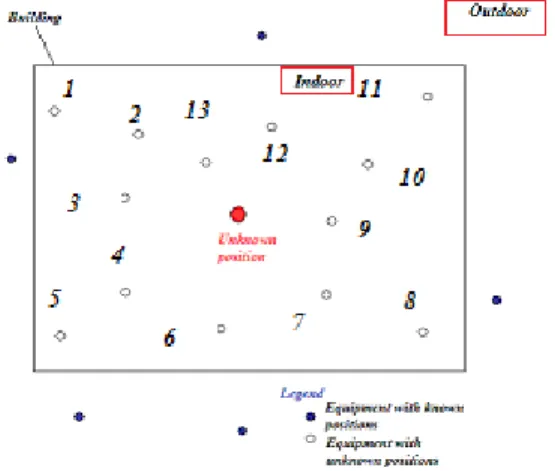
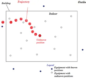
consideration the points that are able to detect all the surroundings nodes equipped with radio waves emitters and receivers. The data needed are tables with lists of detected points that at first are considered as direct neighbors. Tables are extracted from the mobile.

Figure 2 Distribution of mobile equipments The mobile at an unknown position, in figure 2,

According to the theoretical bases described

The graph depends on an essential criterion. In

I.3 RESULTS

To show the results of the approach above, we

In figure 3, we describe the mobile equipment detects all the possible mobile equipments in its neighborhood, and then establishes the adjacency table. For each mobile with known position, a request is send to attribute a table of adjacency for each node with known position.

below, the graph can be built from theses tables. The tables can be considered as lists of adjacency whose entry i give the list of neighbors of vertex i. From these lists we can determine the matrix and the resulting graph.

fact, the distribution of the mobile equipments with the known positions is essential to increase the accuracy of the final results. The best situation is when all the mobile equipments are distributed all around the building for example.

take in consideration only few types of equipment in the network. This limitation is due to simplify calculation for better comprehension.

(5)

Figure 3 Distribution of mobile equipments

(7)

The matrix A represents the spatial relations indoors and outdoors

⎟

⎠

⎞

⎜

⎝

⎛

=

0

1

0

1

0

1

0

1

0

1

0

1

0

1

0

1

0

1

0

1

0

1

0

1

0

1

0

1

0

1

0

1

0

1

0

1

0 A

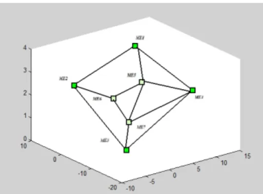
between the nodes of the environment, represented in figure 4. The graph related is shown as:

Figure 4 Graph of adjacency

⎟

⎠

⎞

⎜

⎝

⎛

=

4

0

3

0

3

0

4

0

3

0

3

0

3 D

(8)

⎟

⎠

⎞

⎜

⎝

⎛

−

=

4

1

0

1

0

1

3

1

0

1

0

1

0

3

1

0

1

0

1

4

1

0

1

0

1

3

1

0

1

0

1

3

1

0

1

0

1

3 L

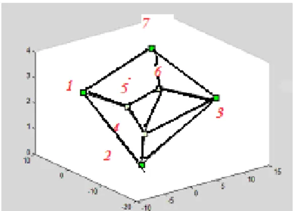
(9) ⎟⎟ ⎟ ⎟ ⎟ ⎟ ⎟ ⎟ ⎟ ⎟ ⎠ ⎞ ⎜⎜ ⎜ ⎜ ⎜ ⎜ ⎜ ⎜ ⎜ ⎜ ⎝ ⎛ − − − − − − − − − − = ′ 1 28 . 0 0 25 . 0 28 . 0 0 0 28 . 0 1 33 . 0 0 0 33 . 0 0 28 . 0 0 1 28 . 0 0 0 0.33 -0.25 -0 0.28 -1 0.28 -0 0..28 -0.28 -0 0 0.28 -1 0.33 -0 0 0.33 -0 0 0.33 -1 0.33 -0 0 33 . 0 28 . 0 0 -0.33 1 L (10)

We change the labels of the mobile equipments as shown in figure 5, in order to obtain another matrix with spatial relations.

(6)

Figure 5 Graph of adjacency

⎟

⎠

⎞

⎜

⎝

⎛

=

0

1

0

1

0

1

0

1

0

1

0

1

0

1

0

1

0

1

0

1

0

1

0

1

0

1

0

1

0

1

0

1

0 A

(11)

⎟

⎠

⎞

⎜

⎝

⎛

=

3

0

3

0

3

0

4

0

4

0

3

0

3 D

(12)

⎟

⎠

⎞

⎜

⎝

⎛

−

=

3

1

0

1

0

1

3

1

0

1

3

1

0

1

0

1

4

1

0

1

0

1

4

1

0

1

3

1

0

1

0

1

3 L

(13) ⎟⎟ ⎟ ⎟ ⎟ ⎟ ⎟ ⎟ ⎟ ⎟ ⎠ ⎞ ⎜⎜ ⎜ ⎜ ⎜ ⎜ ⎜ ⎜ ⎜ ⎜ ⎝ ⎛ − − − − − − − − − − − = ′ 1 33 . 0 0 0 28 . 0 0 33 . 0 33 . 0 1 33 . 0 28 . 0 28 . 0 0 0 0 33 . 0 1 28 . 0 0 0 0.33 -0 0.28 -0.28 -1 0.25 -0.28 -0 0.28 -0.28 -0 0.25 -1 0.28 -0 0 0 0 0.28 -0.28 -1 0.33 -33 . 0 0 33 . 0 0 0 -0.33 1 L (14)

As described in the previous section, the spectral radiuses of the spatial matrix allow us to have the certitude that there is not errors on the matrix and that we are working on the same environment. The two values obtained respectively are ρ (L) = 5.4267 and ρ (L) = 5.4142. Values are very close and the E [ρ (L)] = 6 =n-1, knowing that n represents the size of the matrix or the number of mobile equipments. The last property informs us that the graph is complete. To verify that the graph doesn’t contain loops, the proper values must be equal to zero [3].

I.4 THREE DIMENSIONAL MODEL I.4.1 THEORETICAL APPROACH

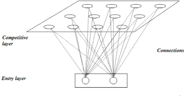
The approach developed here is based on the KOHONEN model. The KOHONEN analysis is a method of unsupervised classification. The self organizing maps of Kohonen consist of a grid. In each node of the grid is a neuron. Each neuron is connected to a reference vector that defines the data space; these vectors represent a discrete representation of the entrance space. They are defined in that manner to retain the initial topology of the nodes. In addition, they keep the neighborhood relations in the grid. They allow to an easy indexing, using the coordinates in the grid. All these features are useful to the visualization of multimensional data.

More in details, after a random initialization of the values of each neuron, neurons are subjected to the self adaptive map. According to the values of the neurons, there is one best suited to the stimulus: One whose value is closest to the data presented. Then this value attributed to this neuron is changed to be more adaptative. Adequate values are attributed to the neighborhood taking a factor lowest than one. Thus, the entire region of the map around the

(7)

winner neuron is specialized. At the end of the algorithm, when the neurons cannot move, self organizing map covers the entire topology of the data.

Figure 6 KOHONEN principle

The mapping of the entrance is achieved by adjusting the vector wr of reference. The adjustment is made by a learning algorithm which is based on a competition between neurons and the importance of the concept of neighborhood. Principle of the algorithm is described in figure 6.

A sequence of random input vectors is presented for learning. With each vector, a new adaptation cycle is started. For each vector v in the sequence, we determine the winner neuron, i.e. the neuron whose reference vector v approach the best: wr v A r v S − ∈ = =

φ

( ) argmin (15)

The winner neuron s and its neighbors (defined by a function of belonging to the neighborhood) move their reference vectors to the input vector.

wtr

+1

=

+

Δ

(16) With

)

(

*

h

v

_wtr

wtr

=

−

Δ

ε

(17) With

ε

=

ε

(t

)

,

( s

r

h

=

defining the learning coefficient and the function defining the neighborhood appurtenance.

)

t

The coefficient of learning defines the degree of the global movement of the map.

I.4.2 PRACTICAL APPROACH

In our case, the Kohonen approach lets us define a certain number of stages for the graph. The acquainted graph to model the environment can be more detailed with learning information about the classification of the nodes that are located at the same or neighbors’ level of altitude. Our study is based on defining the entrance vector as a vector with the directional information and not the distance one. The Kohonen algorithm is based on a distance algorithm between nodes. In our model graph, distances between nodes are not yet calculated.

The objective of our algorithm is to classify all the nodes that belong to the same level of altitude. This classification is a relative classification that can represent an advantage to the final calculation of all coordinates.

For each entrance vector, we define:

)

arg(wr

r =

ϕ

(18)

The winner node is the node that satisfies:

ϕ

φ

_r

A

r

v

S

−

∈

=

(

)

arg

min

(19)

The winner neuron s and its neighbors (defined by a function of belonging to the neighborhood) move their reference vectors to the input vector.

ϕ

t_r+1= t_r+Δ t_r (20) With ) ( *

ϕ

ε

ϕ

t_r= h − t_r Δ (21)

The difference between the classical approach and our approach is that we use the argument of the vector and the measure.

(8)

0 0.2 0.4 0.6 0.8 1 0 0.1 0.2 0.3 0.4 0.5 0.6 0.7 0.8 0.9 1

Figure 7 KOHONEN application

Figure 7 shows the application of the KOHONEN principle on the graph obtained, before. The bases of the KOHONEN algorithm consist to study the attributes of the different mobile points, in order to obtain a model more realistic of the points’ distribution.

I.5 TRAJECTORY

The objective of this study is a general vision of a trajectory for any mobile equipment between a start time and a final time. Based only on adjacency tables of the mobile equipment, the group of acquainted data can be attractive to give a form for the trajectory established without a real position. A database can be obtained with these tables that can enrich the localisation system and make the result more accurate. This type of study can be the very interesting to give all the possible transition in an environment. This point can be a real advantage for the three dimensional positioning.

To establish a real time trajectory many factors are essential.

I.5.1 NOT REAL TIME TRAJECTORY The non real time trajectory is based on a global study of the neighborhood tables. The mobile equipment moves from departure point to the arrival point and acquires all the data of detected points. The tables acquired from the first moment t0 and the last one tn show exactly the migration between detected nodes and so, the migration between the neighborhoods of the mobile point.

To establish this type of trajectory, the time for which we measure the detected points and the velocity of the mobile equipment are necessary factors. The non real time trajectory is not available for short laps of time or for a very slow velocity. We will demonstrate that, later.

Figure 8 Example of trajectory

As shown in the figure 8 below, the trajectory is a collection of successive points. If the mobile equipment can only see its neighborhood and not the neighborhood of the detected points, it can built adjacency tables with only its neighbors. The graph could so be build thanks to a group of tables for the same points but at different moments.

These tables acquired for a certain time can allow us to build a trajectory that can have a local referential and can allow us to establish a learning of the environment.

A certain established number of trajectories acquainted can be useful to:

Build an approximate plan of a building.

Improve the results of a localisation system based on graphics.

I.5.2 REAL TIME TRAJECTORY

A real time trajectory is based on acquainting tables of adjacency for the mobile points and its neighborhood. In fact, the date acquainted for a

(9)

certain laps of time can allow us to build graphs. The very important factors in this real time trajectory are the synchronization and the application time. Synchronization between equipments that are emitters and receivers is necessary. An initial calibration of the system can be achieved, for t=t0.

II. SPATIAL REASONING

The spatial reasoning is considered as a representation and reasoning on spatial entities and spatial relationships. In practice, this science is largely used and developed in the artificial intelligence community and in image interpretation. This type of study can allow us a detailed view of topological characteristics of the space, imprecision representation and management of the neighborhood of chosen point, etc.

In the next paragraph, we describe how to apply this knowledge, combining network data and geographical data to have a representation of the indoor environment.

II.1 THEORETICAL BASES

Spatial reasoning is based on a representation of the space using relations between regions or objects. In what succeed, we are interested on the cardinal relations between objects and directional operators.

The indoor environment is composed by mobile equipment like we describe before. The equipments are divided into two groups. One group includes the mobile equipments with known coordinates; the other group includes the mobile equipments with unknown coordinates. Our approach consists to study relations between all the mobile equipments in the environment. The first step of our research is to study the relation between the known points to establish a table with the directional characteristic of each point. The second step is to use the principles of the routing algorithms combined with an iteration approach to build a complete list of all relations between mobile equipments in the indoor environment.

The direction is defined as a binary relation

between two objects: one represents the reference and the other the target. The last part of a directional relation is the reference frame which assigns names or symbols to the space. This characteristic is related to the reference point taken in consideration. Our study is based on relative relations between mobiles. In fact, each point has a table with relations with each mobile point of the network. The reference point is the mobile point of the table, for which we establish the relations. Tables are not full at the beginning; they are composed by relations between mobile points with known coordinates. Using an iterative approach described below, tables are filled gradually.

Models for the directional relations between spatial objects were developed for 2D space. Recently, researches were conducted to the 3D space. We based our work on this new approach. Directional models are appropriate for an arbitrary distribution of mobile points, based on a separate examination of directional relationships with respecting the three coordinate axes. For each axe, we have two possible relations.

Different approaches were developed for the spatial relation between 3D objects. The major point taken in consideration was the shape of the objects to define relations.

In our case, the mobile equipments are supposed as points. The shape is not taken in consideration. In this approach, the reference object is extruded along the coordinate axis corresponding to the directional operator. The target object is tested for intersection with the extrusion. Let “A” be the reference point with coordinates (ax,ay,az) and “B” the target point with coordinates (bx,by,bz), we have the relations below:

b x

a x

b z

a z

b y

a y

bwith

a

B

A

proj

westOf

b x

a x

b z

a z

b y

a y

bwith

a

B

A

proj

eastOf

p

f

:

,

)

,

(

_

:

,

)

,

(

_

=

∧

=

∃

⇔

=

∧

=

∃

⇔

(22)

(10)

b y

a y

bz

az

bx

ax

bwith

a

B

A

proj

southOf

b y

a y

bz

az

bx

ax

bwith

a

B

A

proj

northOf

p

f

:

,

)

,

(

_

:

,

)

,

(

_

=

∧

=

∃

⇔

=

∧

=

∃

⇔

(23)

bz

az

b y

a y

bx

ax

bwith

a

B

A

proj

below

bz

az

b y

a y

bx

ax

bwith

a

B

A

proj

above

p

f

:

,

)

,

(

_

:

,

)

,

(

_

=

∧

=

∃

⇔

=

∧

=

∃

⇔

(24)

These bases let us acquaint information about mobile points on the network, with known coordinates. Due to the arbitrary positions of the mobile points, the spatial relations are restricted to:

b x

a

b

a

_x

B

A

hs

westOf

b x

a x

b

a

B

A

hs

eastOf

p

f

:

)

,

(

_

:

)

,

(

_

∃

∀

⇔

∃

∀

⇔

(25)

b y

a y

b

a

B

A

hs

southOf

b y

a

b

a

_y

B

A

hs

northOf

p

f

:

)

,

(

_

:

)

,

(

_

∃

∀

⇔

∃

∀

⇔

(26)

b z

a z

b

a

B

A

proj

below

b z

a

b

a

_z

B

A

proj

above

p

f

:

)

,

(

_

:

)

,

(

_

∃

∀

⇔

∃

∀

⇔

(27)

ons between points with nown coordinates.

ns of

with known coordinates are

outdoors.

Relations described above are necessary to determine the relati

k

II.2 PRACTICAL APPROACH

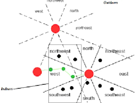
Spatial relations between points are saved in tables. At the beginning of the algorithm, the tables are not full. In fact, at first we have only the spatial relations between nodes with known coordinates. Slowly the tables are filled thanks to data acquainted by examining the relatio mobile points without known coordinates. Before describing the steps of the system, we describe below the principle using figures and nodes distributed randomly indoors. Mobile equipments

Figure 9 Spatial approach

ng algorithm, escribed in the next paragraph.

rdinates included in a margin of values defined.

As shown on figure 9, the mobile points are included in a west space of the mobile point with known coordinates. The suitable path from one node to another in the network is calculated thanks to the Ad-Hoc routi

d

From this type of study, we can obtain tables for each node of the network with spatial relations. These tables allow us to combine results and try to have a certain model of the environment with intersections between regions of each known point. This intersection allows us to have values of the coo

Figure 10 Application of the approach

ons could e different from one point to another.

The spatial relations described in the approach are relations related to the reference object taken in consideration and not geographical absolute directions. Figure 10 shows that directi

(11)

II.3 ROUTING ALGORITHM

Spatial relations between mobile points give us a representation of the space using intersection regions. To define which mobile equipment is attributed to which region, we decide to implement a routing algorithm that could define a certain number of possible routes. These paths allow us to build a database with the mobile

alled proactive due to its

uence numbers are well as for

Our application of this protocol is limited by the one hop nodes.

points not positioned and their regions.

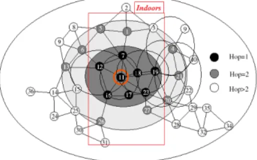
The routing algorithm taken in consideration is based on the protocol Fisheye State Routing “FSR”. Nevertheless, the bases have some differences. Fisheye State Routing is a table-driven or proactive routing protocol. The nodes of a network are characterized by a table with all possible paths to transmit information to another node. The protocol is c

periodical calculation of the routes and that before send a request.

As mentioned, FSR is based on link state routing and it is able of immediately providing route information when needed. FSR maintains a full topology map at each node. The link state packets are exchanged periodically instead of event driven which allow the network to have information about the state of the connection between nodes. The topology tables are sending to local neighbors only. Seq

used for entry replacements as providing loop-free routing.

Figure 11 FSK principle

In figure 11, we apply the principle of our algorithm.

the

d precision when the distance increases (in hop). III. PROPAGATION METHOD

roximate distribution of the mobile equipments.

ngth of the signal, give reliability to the method.

The classical propagation is as follows: Each node is characterized by the one hop region. The path from the sender and receiver is given by the intersection of the one hop regions going from node to node. The chosen path is shortest one looking at the number of hope. In the context of routing, the approach of "fisheye" materializes, for a node, the maintenance of data regarding the accuracy of the distance and quality of the path of a direct neighbor, with a gradual reduction, detail an

In order to improve the calculation of the position, we employed the propagation method. Graphs allow us to have a model of the environment and an app

Combining the spatial representation and the calculation of the distances with the stre

2

4 ⎟

⎠

⎞

⎜

⎝

⎛

=

d

r

G

t

G

t

P

r

P

π

λ

(28)

the distance d through the following formula:

Pr and Gr are the received power and antenna gain, Gt and Pt transmitted power and antenna gain, signal and the l wavelength distance between the transmitter and receiver. Since the measure is typically a received power, it is possible to obtain

r

In the case of the indoor environment, this formula is slightly ch

P

r

G

t

G

t

P

d

π

λ

4 =

(29)

anged and the propagation model is as follows: n

d

r

G

t

G

t

P

r

P

⎟

⎠

⎞

⎜

⎝

⎛

=

π

λ

4

(30)

(12)

The theory has defined the variable as being equal to 2.8 for the external environment. Our previous work and experiences allow us the choice of the variable n as equal to 3.5 for a

o mathematical bases and

f signal strength or

e accuracy and reliability to

IOGRAPHY NC-aches", s and applications, NC-GNSS 2008, i 2008, France. better result [4].

CONCLUSION AND PERSPECTIVES Our research below is based on an approach taking in consideration the relations between mobile equipments. In fact, the environment is modeled by 2D or 3D graphs. These graphs are established thanks t

routing algorithms.

Results acquainted are promising and let us think of innovative method for indoor localisation, that does not need the measures o

time of arrival of the signal.

Perspectives for this approach could be to establish a real complete model of any environment using spatial relations. The main goal is to give mor

positioning results. BIBL

1. Nel Samama, Alexandre Vervisch-Picois, "Current Status of GNSS Indoor Positioning Using GNSS Repeaters ", E GNSS 2005, Munich, July 2005, Germany. 2. Nabil Jardak, Nel Samama, " Future GNSS signals and indoor positioning : multi-constellation and multi-frequency appro GNSS 2007, Genève, Mai 2007, Suisse.

3. E. D. Kaplan and C. Hegarty, Understanding GPS: Principle

Artech House, 2nd ed., 2006.

4. Magda Chelly, Adel Ghazel, Riadh Tebourbi, Nel Samama, “WiFi Hybridisation with Pseudolites and Repeaters for Indoor Positioning Purposes”, E