HAL Id: hal-00948861
https://hal.archives-ouvertes.fr/hal-00948861
Submitted on 3 Mar 2014HAL is a multi-disciplinary open access
archive for the deposit and dissemination of sci-entific research documents, whether they are pub-lished or not. The documents may come from teaching and research institutions in France or abroad, or from public or private research centers.
L’archive ouverte pluridisciplinaire HAL, est destinée au dépôt et à la diffusion de documents scientifiques de niveau recherche, publiés ou non, émanant des établissements d’enseignement et de recherche français ou étrangers, des laboratoires publics ou privés.
Turbidimeter based on a refractometer using a
charge-coupled device
Bo Hou, Philippe Grosso, Zong Yan Wu, Jean-Louis de Bougrenet de la
Tocnaye
To cite this version:
Bo Hou, Philippe Grosso, Zong Yan Wu, Jean-Louis de Bougrenet de la Tocnaye. Turbidimeter based on a refractometer using a charge-coupled device. Optical Engineering, SPIE, 2012, 51 (2), pp.023605. �10.1117/1.OE.51.2.023605�. �hal-00948861�
A turbidi-meter based on a refractometer using a Charge-Coupled Device B. Hou,a) P. Grosso, Z.Y. Wu, and J.L. de Bougrenet de la Tocnaye
T´el´ecom Bretagne Optics Department Technopˆole Iroise 29238 Brest, France
Salinity and turbidity are two important sea water properties in oceanography. We have studied the use of a high resolution refractometer to measure the salinity of sea water. The requirement of a multifunctional sensor makes the turbidity measurement based on our refractometer valuable. In this paper, we measure turbidity according to the attenuation of the laser beam caused by the scattering. With the configuration of our refractometer, several issues impact the laser beam attenuation measurement, while the measurement of salinity is impacted by the scattering as well. All these is-sues make light distribution non-sensitive sensors such as PSD unsuitable for building the refracto-turbidi-meters. To overcome these issues, a CCD combined with a new location algorithm is used to measure both the refractive index and the attenuation. Several simulations and experiments are carried out to evaluate this new method. According to the results, the way to improve the resolution is discussed as well. The validation of our method is proved by comparing to the nephelometer specified by the NTU standard.
Keywords: Charge-Coupled Device, turbidity, turbidi-meter, formazin, refractometer
I. INTRODUCTION
The turbidity of water is mostly due to the existence of suspended undissolved solid particles. When light is incident on a particle, several processes occur, including reflection, refraction, diffraction and absorption. For particles that are of the order of the wavelength in size or smaller, these processes are referred to as “scattering”.1 Usually, the
measure-ment of turbidity is not a direct measuremeasure-ment of these suspended particles, but rather a measurement of the scattering caused by these particles. International standard ISO 70272
provides two different methods to measure the turbidity by computing the diffuse radiation and the attenuation of a radian flux. Respectively, two different turbidity units, namely FNU (Formazin Nephelometric Unit) and FAU (Formazin Attenuation Unit), are used for both methods. Another turbidity unit, Nephelometric Turbidity Unit (NTU), defined by EPA method 180.13 measures the light diffused at an angle of 90 ± 30 degrees to the incident
light beam with a tungsten lamp.
Since the measurement of turbidity is a measurement of the scattering effect caused by particles, the light scattering and its application have been investigated for many years. In 1907, Gustav Mie4 gave an analytical solution of Maxwell’s equations for the scattering
of electromagnetic radiation by a single spherical particle, which is called Mie theory. To reduce the complexity of Mie theory, several approximations have been proposed.5–7
The study of oceanography requires different high-resolution measurement equipment to measure different physical quantities of the sea water, e.g. turbidity, salinity, temper-ature, and pressure, etc.8 A set of these quantities at different geographical positions is
most valuable for oceanography. This makes the research of in situ multi-sensors valuable. Our previous work involved developing an optical refractometer to measure the salinity of seawater based on laser beam deviation measurement with a 1-D Position Sensitive Device (PSD)9,10. The resolution for measuring salinity reaches 0.002g/kg with the measurement
range from 0g/kg to 40g/kg. Further researching to replace PSD with Charge-Coupled Device (CCD) gives us an improvement of resolution of nearly 1.5 times compared to PSD-based refractometer.11The CCD records the location, shape, and intensity distribution of the
laser spot. This provides the possibility to measure physical quantities other than refraction index.
A B C D E F G H O N xp M x′ p water L
FIG. 1. Principle of the refractometer. Dotted line shows the laser path according to two different refraction indices of water
A brief summary of our optical refractometer is given in the next section. In section III, the problems of measuring turbidity with our optical refractometer are discussed according to the scattering theory. Solutions are also introduced in this section. The simulations and experiments are firstly carried out in a parallel slab to operate at normal incidence and then with our optical refractometer, which can be found in section V and VI. Finally, the performance in highly turbid case and calibrated water samples are given by a series of experiments.
II. PRINCIPLE OF OPTICAL REFRACTOMETER
Our optical refractometer used for salinity measurement is depicted in Fig. 1. The refractometer consists of two prisms with different refractive indices. The laser beam first illuminates the left hand side prism and reaches a mirror AB. After the reflection at AB, the laser beam is redirected to the surface between the medium and the prism, CD. It is then refracted and propagates a distance d in the medium. The laser beam is then refracted at surface DE and enters the right hand side prism. The mirror FG finally reflects the laser beam to the top of the prism, where a laser beam position detection device is used to detect the position of the laser spot xp. With this configuration, the refractive index of the water
can be calculated very accurately from the position of the laser spot.9 With a CCD instead
of a PSD, the position of the laser spot can be calculated with different location algorithms, and it is shown that the resolution is comparable to the system that uses a PSD.11By using
a CCD, the distribution of the light intensity changed by the scattering of the particles in the medium is also recorded, giving us the possibility to retrieve the turbidity of the medium.
III. PRINCIPLE OF TURBIDITY MEASUREMENT
A. Theoretical aspects
The incident light is diffused in all directions when it meets the particle. The portion of light flux diffused in different directions is defined by the phase function, denoted as p(ˆs′
, ˆs), which represents the portion of light flux diffused from direction ˆs to direction ˆs′
. The phase function is related to the wavelength of the incident light and the size of the particles, a normalized radius R = 2πr
λ is introduced to define the size of the particle, in
which r is the radius of the particle and λ is the wavelength of the incident light. Besides the flux diffused, another portion of light flux is absorbed by the particle, represented as σaI0, where I0 is the flux intensity of incident light. Similarly, the portion of light diffused
out of the light propagation direction, which is related to the normalized radius R of the particle is denoted as σdI0. Here σa and σd are called absorption cross section and diffusion
cross section, respectively, which are the functions of the incident light wavelength λ. These two coefficients associated with the phase function describe the optical properties of a single particle. For a volume of water, the density of particles should also be considered. The more particles in the medium, the more light is absorbed and scattered out of the propagation direction.
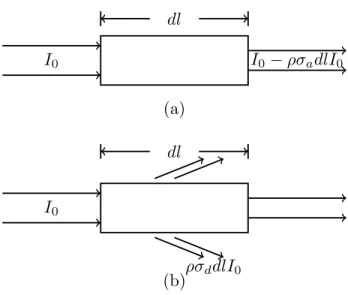
Fig. 2 shows the absorption and diffusion of an incident light with flux intensity I0, upon
a volume of turbid water with unit cross section, particle density ρ and length of dl. The flux that is absorbed by ρdl particles is calculated by the equation:
Ia= ρσa(λ)dlI0 (1)
The portion of light diffused out of the propagation direction by these particles can be expressed by:
Id= ρσd(λ)dlI0 (2)
I0 I0− ρσadlI0 dl (a) I0 dl ρσddlI0 (b)
FIG. 2. The light absorption and diffusion in a unit volume of turbid water. The sub-diagram (a) shows the light with power of ρσadlI0 is absorbed. The sub-diagram (b) shows that the light with
power of ρσddlI0 is diffused out of the propagation direction
is:
dI
dl = −
(Ia+ Id)
dl = −ρ(σa(λ) + σd(λ))I (3)
This partial differential equation can be easily solved as: I = I0e
−ρ(σa(λ)+σd(λ))l
, (4)
in which the part ρ(σa(λ) + σd(λ)) that causes the attenuation of the incident beam, is a
good candidate to describe the optical properties of the volume of medium. To simplify the formula, ρ(σa(λ) + σd(λ)) is expressed as T , attenuation coefficient. Therefore, the
attenuation coefficient T can be calculated from:
T = −ln(Im) − ln(I0)
l , (5)
where Imis the light intensity measured in the transmission path out of the volume. Besides
the attenuation of the incident beam, the light that propagates through the volume of medium increases as a portion of the light flux from other directions are scattered into the transmission direction. This phenomenon is depicted in Fig. 3. Different from the attenuation of the incident light, this part of flux, caused by the multi-scattering in the medium increases the transmitted radiation in the transmission direction, noted as Ims,
I0
dl
FIG. 3. The light scattered from other parts of the medium to the incident light propagation direction
which can not be easily separated from the penetrated light Im. Thus, the Eq. 5 should be
T = −ln(Im− Ims) − ln(I0)
l (6)
Another part of multi-scattering light that increases the transmission radiation is caused by the reflection between the two refraction surfaces. Besides the refraction, a part of the laser beam is reflected in the second refraction surface, the reflected light is diffused by the particles in the medium and reflected again in the first refraction surface. This process continues between the two surfaces. As a result, part of the reflected light is scattered into the transmission direction as well.
The flux intensity of multi-scattered light in propagation direction is related to the density of the particles and the length of the light path. The higher the density of the particles, the more multi-scattering occurs. A longer light path gives more light scattered into the propagation direction too. In this paper, the impacts caused by the multi-scattered light are evaluated in the analysis of the experiment results.
B. The resolution of turbidity measurement
The resolution of the turbidity measurement can be estimated from the Eq 6. The multi-scattering part is ignored here and will be discussed later from the experiment results. Since the incident light intensity I0 can be measured with non-turbid water in advance, the
equation can be modified as:
T = −(ln(Im)
l − C) (7)
The derivative of T can be expressed as: T′ = dT dIm = − 1 l × Im (8)
Thus, the sensitivity of the measurement of turbidity St is
St= kt× dT = −
dIm
l × Im
, (9)
where kt is a constant coefficient to convert the attenuation coefficient into other turbidity
units, for example, NTU. From this equation, it is obvious that the resolution of turbidity measurement is proportional to the resolution of the light intensity sensor dIm, but inversely
proportional to the length of the light path l in the turbid medium. A longer light path can provide better turbidity measurement resolution. Another interesting phenomenon re-sulting from this equation is the resolution depending on the measurement range. With the same sensitivity of the light intensity sensor and the same light path length, the larger the measured intensity, the better the resolution obtained. Considering that the measured light intensity decreases as the turbidity increases, it is easy to conclude that the resolution is better in low turbid medium than in the high turbid medium when light path and sensor sensitivity are the same.
C. Issues in measuring turbidity with refractometer
As discussed in section III, the attenuation coefficient T can be calculated from the attenuation of the incident laser beam according to Eq. 6. When applying this theory to the refractometer demonstrated in section II, several issues arise. The first one is, according to the theory, the intensity Im is measured by the sensor located far away from the medium,
where the light in propagation direction is well separated from the scattered light, however, with the refractometer, the height L shown in Fig 1 limits the distance between the sensor and the medium, making it difficult to measure the separated light beam intensity. Fig. 4 depicts the difference of light intensity measurement while locating the light intensity sensor at different distances of the medium. Besides the light propagated along the transmission direction, another portion of light is scattered out of the medium. The sensor located near the medium, shown in position A, captures not only the transmitted radiation but also the scattered radiation with an angle α, while at the distant position B, the sensor accepts the transmitted radiation and the scattered radiation with the angle β, smaller than α. Therefore, B receives less scattered light than A.
Besides the difficulty of separating the scattered radiation and the transmission radiation, the use of laser as the source leads to interference while the laser beam propagates through
A
B
water
I
0α
β
FIG. 4. The difference of light intensity measurement by locating the light intensity sensor at different distances of the medium
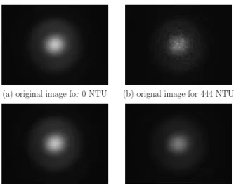
the particles. As a result, speckle is observed in the sensor plane. Fig. 10 (a) and (b) show the laser spots captured at 5 cm far from the medium along the light propagation path. Picture (a) depicts the laser spot with pure water and picture (b) shows the laser spot with the turbid water of 444.4 NTU. It is obvious that the laser spot captured with turbid water mixes the Gaussian spot and interference speckle. Both the scattered part of flux and the speckle created by the interference cause inaccurate measurement of turbidity, and need to be eliminated.
Furthermore, since our method measures the attenuation of propagated light as shown in Eq. 6, it is easy to find out that the light intensity Im decreases when the turbidity
increases, which can be found by comparing the Fig. 10 (a) and (b). This results in another issue, the light intensity becomes so weak that it can’t be measured in a highly turbid case. Another problem raised by the refractometer is that the light path changes as the re-fraction index of the medium changes. In Fig.1, OM and ON are two different light paths according to different refraction indices of the medium. This makes the measured flux in-tensity quite different when measuring two different medium samples, which have the same turbidity but different refractive indices. According to the configuration of the refractome-ter, the light path length in the medium named l in Eq.6 can be expressed as a function of the laser spot position, which is shown in Fig. 5. The laser spot position is counted from the H point shown in Fig. 1. A quadratic fitting gives us an approximate equation to calculate the length of light path according to the laser spot position, which is expressed in Eq. 10.
l = f (xp) = 6.338340 − 0.000284 xp+ 0.000185 x2p (10)
6.34 6.35 6.36 6.37 6.38 6.39 6.4 7 8 9 10 11 12 13 14 15 16 17 18
length of the light path in the medium (mm)
laser spot position (mm) Light path length vs spot position
FIG. 5. The relationship between the length of the light path in the medium and the laser spot position. The laser spot position is the distance from the H to px in Fig.1
O
M
O
′M
′FIG. 6. Different parts inside the beam pass different lengths in the medium
pure water is calculated and used as the length in Eq. 6 to obtain the attenuation coefficient. In practice, the laser beam width cannot be ignored. This leads to another problem, the width of the collimated beam causes that the different parts inside the beam propagate through the medium with different lengths. As shown in Fig. 6, for a wide beam shown as the red, the upper parts of the beam have shorter light paths OM than the bottom of the beam O′
M′
, and this difference varies as the refractive index of the medium changes. A solution to this problem is to use the maximum of the intensity, instead of the entire intensity, to calculate the attenuation coefficient T .
The above problems raised by the configuration of the refractometer impact the resolution of the measurement of turbidity. Meanwhile, the measurement of turbidity itself impacts the accuracy of the refractometer, which needs to be addressed in the design of the turbidi-meter. The first problem related to the resolution of the refractive index measurement is caused by the light path difference as shown in Fig. 6. According to Eq. 6, in a turbid case, this difference of light path leads to different attenuation inside the laser spot, which further causes the change of the laser beam position when applying the mass-center-related laser
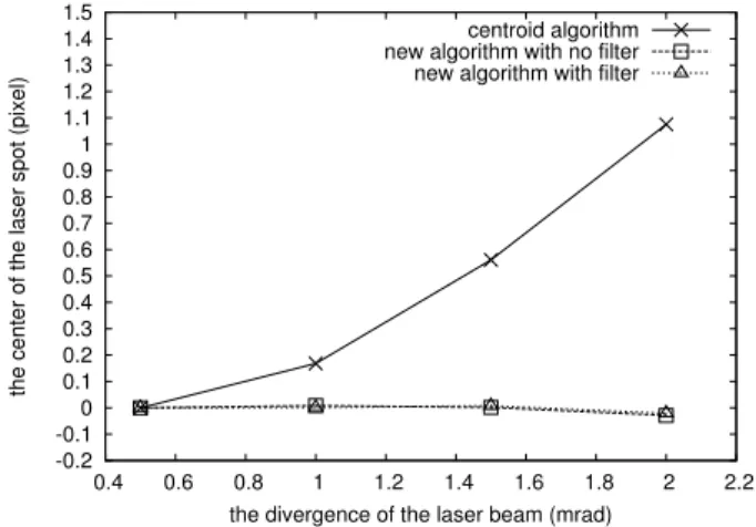
spot location methods, for example, using PSD or CCD combined the centroid algorithm. Another problem that leads to the asymmetric laser spot is the divergence of the laser beam. Both the refraction surface and the sensor surface are not perpendicular to the laser beam. When a Gaussian beam projected to the sensor surface at a non-normal angle, the Gaussian spot becomes asymmetric, while different refractive index changes the size of the laser spot. Fig. 7 is generated by the simulation in ZEMAX with the configuration of our refractometer. It presents four laser spots with different laser beam divergences, but with the same refractive index of the medium. It is easy to observe that the width of the laser spot increases as the divergence of laser spot increases. The asymmetry of the laser beam can be noticed from the center of these laser spots calculated by the centroid algorithm, which is depicted in Fig. 8 (The solid line with mark ‘x’). The center of the laser spots moves more than 1 pixel from the divergence of 0.5 mrad to 2 mrad.
Similarly with the divergence of the laser beam, the turbidity of the medium diffused the laser beam out of its propagation direction and makes the divergence of the laser beam much larger. Fig. 9 is the result of the simulation in ZEMAX with the collimated laser beam (no divergence) and different densities of particle. The scattering model used in the simulation is the Mie scattering. It is noticed that the position calculated by the centroid algorithm has a deviation of 2.5 pixels with the particle density from 0/cm2 to 8 × 10⁶/cm2.
D. Using CCD to measure the turbidity with a refractometer
One of our previous work used a PSD to measure the deviation of the laser beam. PSD has a single active area formed by a P-N junction. The two parts that originated from the laser spot to the two electrodes form two lateral resistances for the photo-currents running towards the electrodes. The photo currents are collected through the resistances by the output electrodes, which are inversely proportional to the distance between the electrode and the center of the incoming light beam. This relationship is expressed as follows:12
x = L
2
I2− I1
I2+ I1
, (11)
where I1 and I2 are the electrode photo-currents, L is the length of the PSD active area and
x stands for the laser spot position. From the principle of PSD, the light intensity can be calculated from I1 + I2. However, since PSD is placed not far from the medium due to the
(a) divergence of 0.5 mrad
(b) divergence of 1.0 mrad
(c) divergence of 1.5 mrad
(d) divergence of 2.0 mrad
FIG. 7. The laser spots for different laser beams with different divergence. The image is obtained from the ZEMAX simulation.
dimension limitation of the prisms, the intensity it measures mixes the scattered radiation so that it cannot give an accurate result. From the principle of PSD, the center is the mass center of the incident light. Since the divergence and turbidity make the laser spot asymmetric, the mass center cannot be used to indicate the laser beam position. What is more, when the light intensity is very weak in a highly turbid medium, I1 and I2 will be so
small that they cannot be retrieved. These problems, which exist for all the light intensity distribution insensitive sensors make the PSD a poor candidate to measure turbidity with the refractometer.
-0.2 -0.1 0 0.1 0.2 0.3 0.4 0.5 0.6 0.7 0.8 0.9 1 1.1 1.2 1.3 1.4 1.5 0.4 0.6 0.8 1 1.2 1.4 1.6 1.8 2 2.2
the center of the laser spot (pixel)
the divergence of the laser beam (mrad) centroid algorithm new algorithm with no filter new algorithm with filter
FIG. 8. The positions obtained by the different algorithms for different divergence of laser beam. (simulated in ZEMAX) -0.5 0 0.5 1 1.5 2 2.5 3 0 1 2 3 4 5 6 7 8
the position calculated
particle density (M)
centroid algorithm new algorithm
FIG. 9. The positions obtained by the different algorithms for different density of particles in the medium. (simulated in ZEMAX)
the deviation of laser beam with CCD combined with a centroid algorithm has been proved to be better than the configuration with PSD.11 Since CCD can be controlled to operate
with different exposure times, the transmitted radiation in a high turbid medium can be measured with high exposure time. The attenuation coefficient T can be represented by calculating with the transmitted radiation in a unit time period, which can be expressed as:
T = −ln( Im t ) − ln( I0 t0) l(xp) , (12)
in which t is the exposure time and t0 stands for the exposure time used to measure the
(a) original image for 0 NTU (b) orignal image for 444 NTU
(c) image after filter for 0 NTU (d) image after filter for 444 NTU
FIG. 10. (a) the original image with pure water (b) the original image with turbid water of 444.4 NTU (c) the resulting image with pure water after passing through the low pass filter (d) the resulting image with turbid water of 444.4 NTU after passing through the low pass filter
beam, it is noted as l(xp) according to Eq. 10.
To separate the transmitted radiation with the scattered radiation, the Fourier transfor-mation of the laser spot in different turbidities has been studied, depicted in Fig. 11, and gives us the profile of the laser spot Fourier transformation in pure water and turbid water of 444.4 NTU. Since a laser is used in the refractometer, the ideal Fourier transformation of the laser spot should be Gaussian too, which can be found in the low frequency (between the spatial frequency -20 and 20 approximately). By comparing the Fourier transformation for different turbidities in Fig. 11, a low pass filter can be used to remove the scattered radi-ation. The result of a low pass filter can be found in Fig. 10 (c) and (d). For pure water, the resulting image does not differ much from the original image, which can be foreseen since there is no scattering in this case. The image (d) shows that this method correctly retrieves the original Gaussian spot from the original image that mixed the transmitted radiation, the scattered radiation and the speckles caused by interference. For the wide beam, the max-imum value of the spot is used to avoid the asymmetric spot caused by the different light paths inside the beam. By applying all these settings to Eq. 12, the attenuation coefficient is: T = −ln( If c t ) − ln( I0 t0) l(xp) , (13)
0 0.0005 0.001 0.0015 0.002 0.0025 0.003 0.0035 0.004 -600 -400 -200 0 200 400 600 frequency 0 NTU 444.4 NTU 0 0.0005 0.001 0.0015 0.002 0.0025 0.003 0.0035 0.004 -200 -150 -100 -50 0 50 100 150 200 frequency 0 NTU 444.4 NTU
FIG. 11. The Fourier transformation profile of the laser spot with different turbidities. The upper diagram shows the profiles with pure water (shown in red) and turbid water of 444.4 NTU (shown in blue); the bottom diagram is the zoom of the profiles from -200 spatial frequency to 200 spatial frequency
for one measurement to avoid accidental errors, the attenuation coefficient can thus be obtained by the formula PN1 Ti
N , in which Ti is the attenuation coefficient calculated from
Eq.13 with the ith image.
As discussed in the section III C, the measurement of turbidity and the divergence of the laser beam can cause the laser spot shape to be asymmetric, which leads to the centroid algorithm inaccuracy in showing the position of the laser spot. To solve this problem, a new algorithm is proposed, which is insensitive to the distribution of the laser spot. Fig 12 describes this algorithm, which tracks the peak of the Gaussian source shown as the dash line. This dash line divides the divergent laser beam into two parts, named left part and right part, respectively. Since the source laser beam can be considered as a perfect Gaussian beam, the mass of the left part Mlef t is equal to the right one Mright and this relationship
holds after the refraction of the beam, even though the shape is asymmetric. This beam is quantized into pixels, which is shown as the bars in Fig 12, by a CCD. The mass in the left part M′
lef t can be expressed as:
M′ lef t = i X 0 Pi+ M∆x, (14)
where M∆x is the mass shown as the shadow area, Pi is the value of ith pixel. Similarly,
the right part M′
x i
i − 1
i − 2 j j + 1 j + 2
∆x
FIG. 12. The principle of new laser spot location algorithm
M′ right = width−1 X j Pj − M∆x (15)
With Eq. 14 and 15, the area in the shadow is obtained by
M∆x = Pwidth−1 j Pj − Pi 0Pi 2 (16)
And the sub-pixel position is calculated as:
xp =
M∆x
Pj
+ i (17)
In a turbid medium, the attenuation is not uniform inside the beam. For a standard Gaussian beam f (x) = I0e
−(x−xp)2
2σ2 , after the attenuation, the beam changes to:
I = I0e −(x−xp)2 2σ2 e− T u(x−xp)−T l= e− (x−xp+ T σu2)2 2σ2 I0e T 2σ2 2u2 −T l, (18)
in which T is the attenuation coefficient, l is the light path of the center, u is a coefficient which describes the different attenuation inside the beam, xp is the original peak position,
and σ is the laser beam size. From this equation, it is easy to conclude that the new laser spot is still a Gaussian spot but with a peak shift of −T σ2
u compared to the original spot.
The peak value of the Gaussian spot attenuates to eT 2σ22u2 −T l of the original one.
Thus, the mass of the left part and the right part of peak can be calculated from the following equations:
M′′ lef t = I0 Z xp−T σ2 u −∞ e−(x−xp+ T σ 2 u )2 2σ2 e T 2σ2 2u2 −T ldx = M′′ right = I0 Z +∞ xp−T σ2 u e−(x−xp+ T σ 2 u )2 2σ2 e T 2σ2 2u2 −T ldx (19) As in the divergence case, the center calculated by Eq. 17 is xp− T σ
2
u . To obtain the
laser spot position xp, the deviation part −T σ
2
u needs to be calculated first. To simplify the
discussion, the coefficient σ2
2u2 is noted as v, thus the maximum value measured is I0evT
2−T l
. According to the principle discussed in chapter III, we obtain the following equation:
vT2− T l = ln(Im) − ln(I0) (20)
By solving this equation, the attenuation coefficient T is expressed as:
T = l −pl
2+ 4v(ln(I
m) − ln(I0))
2v (21)
Combined with Eq. 17, 19, and 21, the laser spot position xp in turbid medium is
calculated by: xp = w( M∆x Pj + i) + k(l − pl2+ 4v(ln(I m) − ln(I0))), (22)
where w is the size of the pixel.
IV. NEW ALGORITHM FOR TURBIDITY MEASUREMENT WITH CCD
A. Simulation
To evaluate the performance of the new algorithm, two simulations: divergence simulation and turbidity simulation, are carried out in ZEMAX, in which the configuration of the refractometer is simulated, while the scattering model chosen for the simulation of turbidity is the Mie scattering. The divergence simulation takes 4 images with 4 different laser beam divergences from 0.5 mrad to 2 mrad. The new algorithm is applied to both the original image and the filtered image. The calculated center can be found in Fig. 8. To simplify the comparison, the reference center used here is the center calculated for 0.5 mrad, which labeled as position 0. From Fig. 8, it is clear that the new algorithm obtains better stability
than the centroid algorithm when applying different divergences. Table I gives more detail of the center calculated by the new algorithm, which shows a maximum error of 0.028 pixel.
TABLE I. Center calculated with different algorithms for different divergences Divergence (mrad) 0.5 1.0 1.5 2.0
centroid (pixel) 0 0.1684 0.5612 1.0754 new algorithm without filter (pixel) 0 0.0087 0.0014 -0.0286
new algorithm with filter (pixel) 0 0.0013 0.0078 -0.0205
The turbidity of the medium is simulated by changing the density of the particles. The reference image is the image simulated in non-turbid case here. 4 different particle densities (2×10⁶/cm3, 4×10⁶/cm3, 6×10⁶/cm3, 8×10⁶/cm3) are simulated and the result is depicted
in Fig. 9. Since the turbid medium diffuses the light out of the beam, a threshold is used to eliminate those light intensities that are diffused out of the laser spot but captured by the CCD. Combined with the threshold, the new algorithm provides a much more accurate result than the centroid algorithm, which gives a deviation of 2.4 pixels. In Table. II, the error of the new algorithm can be found as about 0.069 pixel.
TABLE II. Center calculated with different algorithms for different turbidity density of particles (per cm3) 0 × 106 2 × 10⁶ 4 × 10⁶ 6 × 10⁶ 8 × 10⁶
centroid algorithm (pixel) 0 0.6117 1.2273 1.8364 2.4439 new algorithm (pixel) 0 -0.0552 -0.0550 -0.0149 0.0695
B. Experiments
In our last paper11, several experiments were carried out to evaluate the performance
of the centroid algorithm with a mirco-positioner, which can move with a step of 0.1 µm. To compare the performance of the centroid algorithm with the new algorithm, the same image set is chosen, and the two algorithms are applied. The centers calculated by these two algorithms are depicted in Fig. 13. Furthermore, the result for the new algorithm with the filter is included in this figure too. It is obvious that the curve of the new algorithm is much smoother than the centroid algorithm. The error of these methods can be calculated by a
640.5 641 641.5 642 642.5 643 643.5 644 644.5 645 645.5 646 646.5 647 0 10 20 30 40 50
the calculated position
the step of micro-positioner (0.1um) centroid algorithm new algorithm with no filter new algorithm with filter
FIG. 13. The calculated center provided by the centroid algorithm, new algorithm with and without filter.
linear fitting. Centroid algorithm obtains a maximum error of 0.1 pixel with the standard deviation of 0.0784 pixel, while the new algorithm with and without the filter get a maximum error about 0.06 pixel (the standard deviations are 0.0348 and 0.0352 pixel respectively). For an image with M × N pixels, the two algorithms have the same time complexity of O(M N ). All the results above make the new algorithm a good alternative to the centroid algorithm even in non-turbid case. Besides, according to the simulation results and the algorithm analysis, the new algorithm is insensitive to the divergence and can be applied to the turbid medium.
V. SIMULATION & EXPERIMENT IN A PARALLEL SLAB
A. Simulation
To test the principle of turbidity measurement, the simulation in parallel slab are carried out, firstly in ZEMAX. The turbidity of the medium is changed by adjusting the density of the particles from 1 × 10⁶/cm3 to 1 × 10⁷/cm3. The scattering model used in the simulation
is the Mie scattering. The dimension of the parallel slab follows the size of the parallel slab used in the real experiment. A CCD is placed 10 cm from the parallel slab along the laser beam propagation direction. Table III depicts the attenuation coefficient T calculated by Eq 6. By doing a linear fitting, the attenuation coefficient given by the method correctly describes the density of the particles, which is theoretically proportional to the turbidity
in the simulation. The error standard deviation of the calculated attenuation coefficient T according to the line is 8.2 × 10⁻⁴
. This result means the multi-scattered light Ims can be
ignored in Eq 6 due to the short light path in the turbid water.
TABLE III. Simulation results with the parallel slab
density of particles (106/cm3) 0 1 2 3 4 5 6 7 8 9 10
attenuation coefficient 0 -0.015 -0.029 -0.044 -0.059 -0.073 -0.088 -0.104 -0.118 -0.133 -0.150
B. Experiments in high turbid medium
Besides the simulation, an experiment was carried out in the parallel slab. Fig. 14 shows the setup of the experiment. A red diode laser at 635 nm is mounted perpendicularly to the horizontal plane. A 45 degree mirror redirects the laser beam to a parallel slab with a width of 16 mm. Another 45 degree mirror is used to redirect the propagating beam into a DALSA CCD camera13, with a 1280 × 960 resolution and a small 3.75 × 3.75µm pixel
size. The turbidity reference used in the experiment is the 4000 NTU Formazin standard. Since the scattering is sensitive to the size of the formazin particles, which change according to temperature, the setup was established in the presence of a thermostat to keep the temperature stable. To obtain different turbidity, 1 ml 4000 NTU Formazin standard was added N times to the parallel slab, which contained 40 ml pure water at the beginning. The turbidity of diluted turbid water can be calculated by:
ti =
ti−1× Vi−1+ ∆V × 4000
Vi−1+ ∆V
, (t0 = 0, V0 = 40) (23)
where ∆V is the added volume of 4000 NTU Formazin standard each time, ti and Vi is the
turbidity and the total volume after adding the ∆V of 4000 NTU Formazin for ith time. 10 images are captured for each turbidity with a sufficient exposure time to make sure the peak of the spot reaches more than 100 (maximum 255 for the CCD). Since the diluted formazin is not stable for long time storage, all experiments are carried out in a dark room and in less than 1 hour to obtain the best performance.
Fig 15 shows the experimental result. The light intensity I0 is pre-measured with pure
turbid water
mirror mirror thermostat
pure water laser
CCD
FIG. 14. The experiment setup for the experiments carried out in a parallel slab
-2.5 -2 -1.5 -1 -0.5 0 0.5 1 0 50 100 150 200 250
attenuation by different algorithms
turbidity (NTU)
power of the image max value max value from new algorithm
FIG. 15. Experimental results for the parallel slab for high turbid medium.
coefficients are calculated by using the power of the image, the max value of the image, and the pixel value in the position obtained from the new algorithm as Im, respectively. All these
three curves show linearity to the turbidity which is in the range from 0 NTU to about 234.1 NTU as expected. The average error of these three methods is estimated by a linear fitting, which gives three similiar slopes of −0.0085, −0.0084, −0.0086, respectively. By using the max value of the image, the standard deviation of error is the largest of the three, which reaches ±4.87 NTU, while the standard deviation of error obtained by using the power of the image is ±3.17 NTU. The standard deviation of error given by the new algorithm is the smallest: ±2.82 NTU. From Eq 6, it is easy to conclude that the resolution of the turbid-meter is proportional to the sensitivity of the light sensor and inversely proportional to the light path length. It is believed that the resolution in the experiment can be improved by simply extending the width of the slab.
-0.12 -0.1 -0.08 -0.06 -0.04 -0.02 0 0 2 4 6 8 10 12 14 16
attenuation by different algorithms
turbidity (NTU)
power of the image max value max value from new algorithm
FIG. 16. Experimental results for the parallel slab for low turbid medium.
C. Experiments in low turbid medium
As discussed in section III B, the resolution of the turbid-meter is better in the low turbid medium than in the high turbid one with the same light path and light sensor sensitivity. To demonstrate that, another experiment was carried out with the same parallel slab. All the configurations in this experiment are the same as the one for the high turbid medium discussed in the last section. 40 ml pure water is poured into the slab as the base volume of water. 1 ml diluted turbid water with the turbidity of 78.43 NTU is added to the slab 9 times. For each time, 24 images are captured within 1 second. According to Eq 23, the range of the turbidity for the 9 media varies from 1.91 NTU to 14.41 NTU. Fig. 16 expresses the attenuation coefficient calculated by using the power of the image, the maximum of the image and the pixel value given by the new algorithm, respectively. All of them show a linearity with respect to the turbidity. Even in this small range of turbidity, it is clear that the higher turbid medium gives larger error than the low turbid medium. For these three methods, the maximum value gives a large deviation in higher turbidity medium than the other two. The standard deviation of error for the three methods can be estimated by a linear fitting, which shows that the standard deviation of error of using the power of the image is about ±0.5 NTU, while the new algorithm provides a standard deviation of ±0.6 NTU. Compared with the standard deviation of error obtained in the last section, the resolution of the turbidity is better in a low turbid medium than in a high turbid one.
VI. SIMULATION & EXPERIMENT WITH A REFRACTOMETER
A. Simulation
The simulation of measuring the turbidity with our refractometer was carried out in ZEMAX. The turbidity of the medium was changed by modifying the particle density of the medium from 1 ×10⁶/cm3 to 1 ×10⁷/cm3. The divergence of the laser beam is set to 1 mrad,
the same as the source used in the experiment. A CCD of 1280 × 960 pixels is simulated by a rectangular detector. Table. IV expresses the attenuation coefficient calculated from the simulation. Similarly to the parallel slab case, the attenuation coefficient given by the algorithm discussed in this paper shows a good linearity to the density of the particles in the medium, which is theoretically proportional to the turbidity of the medium.
TABLE IV. Simulation results with the refractometer
density of particles (106/cm3) 0 1 2 3 4 5 6 7 8 9 10
attenuation coefficient 0 -0.018 -0.036 -0.053 -0.071 -0.090 -0.107 -0.126 -0.144 -0.165 -0.185
B. Experiments in high turbid medium
Fig. 17 shows the set up of the experiment with the refractometer. The refractometer is used instead of the parallel slab. The diode laser and CCD used in this experiment are the same as those used in the parallel slab experiment. The refractometer is set-up in a small tank, in which 100 ml pure water is used as the base water. 0.5 ml 4000 NTU formazin solution was added to the small tank 11 times and is diluted to different turbid water levels. The turbidity can be calculated according to the Eq. 23. All the experiments are carried out in the presence of a thermostat to make sure the temperature of the turbid medium does not change.
The experimental results are shown in Fig. 18. The attenuation coefficients are calculated by two different quantities, the power of the image and the pixel value given by the new algorithm, as the measured intensity Im in Eq. 21. The reference light intensity I0 is
pre-measured in pure water with the same configuration. As the turbidity increases, both methods give a trend of decrease for the attenuation coefficient. The average error of these two methods can be evaluated by a linear fitting. The method using the power of the image
laser
CCD
turbid water pure water
thermostat
FIG. 17. Experiment setup for the experiments carried out with the refractometer
-2 -1.5 -1 -0.5 0 0 50 100 150 200 250
turbidity indicator by different algorithms
turbidity (NTU)
turbidity indicator (power of the image) turbidity indicator (max value from new algorithm)
FIG. 18. Experimental results with the refractometer in high turbid medium
as the measured intensity provides an error with standard deviation of ±8.09 NTU, while the standard deviation of error for the method using the new algorithm is about ±7.96 NTU. As we have discussed in Section III B, the sensitivity of the measurement of turbidity is inversely proportional to the light path in the medium. Compared to the error obtained in the parallel slab with 15.91 mm, the error obtained with the refractometer fits this analysis. From the Eq. 10, the light path distance can be calculated as about 6.36 mm. The ratio of the errors between parallel slab and refractometer is about 2.7, while the ratio between the light path in parallel slab and the one in refractometer is about 2.5. It is believed that the difference between both ratios is caused by the set-up error of the laser source, which makes the laser beam not exactly perpendicular to the horizontal plane. This set-up error makes the actual light path distance shorter than the theoretical one.
C. Experiments in low turbid medium
The performance of the turbidity measurement with the refractometer in a low turbid medium is tested with another experiment. The experiment set up is the same as the experiment in high turbid medium discussed in last section. 100 ml pure water is used as the base medium, while diluted formazin of 190 NTU is added into the base medium 11 times to generate different turbid water from 0 NTU to about 19 NTU. The attenuation coefficients calculated from the power of the image and the pixel value obtained by the new algorithm are plotted in Fig. 19. The power of the image shows a better linearity than the new algorithm. The reason is that in a low turbid case, the attenuation of the light is very small so that the non-uniqueness of the attenuation inside the beam is not significant. Thus, the more pixels of the spot used as the measured intensity Im, the more accurate the result
is. However, the new algorithm only tracks the intensity in one location, which divides the the mass of the spot into two identical parts. Therefore, it highly depends on the sensitivity of the light intensity sensor. In a low turbid case, the attenuation of the light intensity for one pixel is so small that the CCD cannot detect it, this explains that in the low turbid case shown in Fig. 19, the attenuation coefficient calculated from the new algorithm does not hold a linearity, especially in ultra low turbid mediums. The experimental results with parallel slab prove this as well, in which the standard deviation of new algorithm (±0.6 NTU) is larger than the standard deviation of using the image power (±0.5 NTU). With the refractometer, the standard deviation of using the power of the image is obtained from a linear fitting, which is about ±1.15 NTU. The ratio between this error and the error obtained in the parallel slab (±0.5 NTU) is 2.3, which fits the ratio between the light paths (about 2.5).
VII. COMPARE TO THE NEPHELOMETER
Nephelometer, which measures the diffusion of the light at 90 degree from the light propa-gation direction, is a stationary or portable instrument for measuring suspended particulates in a liquid or gas colloid. It has been proved to be an accurate and reliable method to mea-sure turbidity from scattering. To test the performance of our method mentioned in this paper, the experimental result is compared to the result obtained from a nephelometer. The
-1 -0.8 -0.6 -0.4 -0.2 0 0 2 4 6 8 10 12 14 16 18 20
turbidity indicator by different algorithms
turbidity (NTU)
turbidity indicator (power of the image) turbidity indicator (max value from new algorithm)
FIG. 19. Experimental results with the refractometer in low turbid medium
test sample is 100 ml diluted formazin turbidity solution. The turbidity of the sample is firstly measured in the nephelometer HACH 2100N14, which gives a result of 109 ± 2 NTU.
The experiment setup is the same in section VI B. The turbidi-meter is firstly calibrated by adding 1ml 4000 NTU formazin turbidity solution into 100 ml pure water for 3 times. For each time, 24 images are captured by the CCD within 1 second. Since the test sample is not in low turbid range, the new algorithm is used to calculate the attenuation coefficient. The attenuation coefficients calculated for the calibration are shown in Fig. 20. A linear fitting is made from the calibration results, which has a slope of −0.0055. With this calibrated configuration, the experiment with test sample is carried out as well. The attenuation coef-ficient obtained by the new algorithm is −0.6054. According to the slope of the fitting line, the turbidity of the test sample can be calculated as t = T
k =
−0.6054
−0.0055 = 110.07 NTU, which
fits the result obtained from the nephelometer.
VIII. CONCLUSION
Salinity and turbidity are two important properties of sea water for oceanography. Our previous work has studied a high resolution optical refractometer to measure salinity. The integration of the salinity and turbidity measurement into one compact sensor is a very interesting topic in oceanography. Based on our refractometer, the attenuation of the light intensity caused by the scattering is measured by using a CCD. The attenuation coefficient, which is proportional to the absorption, diffusion, and particle density of the medium, is chosen as the description of the turbidity. According to the analysis of the attenuation
-0.7 -0.6 -0.5 -0.4 -0.3 -0.2 -0.1 0 0 20 40 60 80 100 120 turbidity indicator turbidity (NTU) turbidity indicator
FIG. 20. Experimental results with the refractometer
coefficient computation, the resolution of this method is proportional to the sensitivity of the light intensity sensor, and inversely proportional to the light path in the medium and the measurement range.
With the configuration of our refractometer, the measurement of turbidity has to face sev-eral issues. The interference of the laser is observed in turbid medium, which forms speckles that lead to unexpected result. In our configuration of the refractometer, different refractive index will result in a different light paths. The width of the laser beam and the refraction result in the non-uniform attenuation inside the beam, which disturbs measurement of the attenuation from the laser spot power. In contrast to refractive index measurement, the attenuation measurement requires that the laser intensity is stable during the measurement as a reference intensity. Besides the laser beam, the light diffused out of the beam is received by the light intensity sensor as well, which disturbs the power of the spot. Furthermore, attenuation makes the light intensity too weak to measure, which causes bad performance in high turbid medium. All these problems determine that a simple light instensity sensor such as PSD cannot afford to measure the turbidity in a refractometer. To overcome these problems, a CCD is used to deal with these issues. With recording the light intensity distri-bution, an image captured by CCD can be treated with a low pass filter to eliminate speckle, and the diffused light can be eliminated by applying a proper threshold. The laser intensity is automatically controlled to keep it stable during all the measurement. By playing with a longer exposure time, weak light can be captured as well. To avoid the non-uniform light path inside the laser beam, only one ray of light is traced and used to calculate turbidity.
In addition to the issues of measuring the turbidity with a refractometer, the turbid medium impacts the measurement of the refractive index as well. Due to the convergence of the laser beam, the laser spot becomes asymmetric, when it is captured by a CCD that is non-perpendicular to the laser beam. What is more, turbidity makes this phenomenon much more obvious. Besides the asymmetric of the laser spot, the turbidity results in a shift of the laser spot peak, which is proportional to the attenuation coefficient. This shift needs to be corrected when applying mass-center-based algorithm to locate the laser spot. A CCD records all the distribution information of the laser spot, which makes it possible to retrieve the position information more accurately. A new algorithm, which tracks the location that divides the mass of the spot into two equal parts, is introduced in this paper, and is proved to be more accurate than the centroid algorithm in both the non-turbid environment and turbid environment.
Through the simulations and various experiments, the average accuracy of our method based on the current refractometer reaches 8 NTU in a range from 0 NTU to 200 NTU and 1.15 NTU in a range from 0 NTU to 20 NTU. We compared our method with the nephelometer specified by the NTU standard. The result computed by our method well fits the result obtained from a nephelometer. The sensitivity can be improved by increasing the length of the light path in the medium, which is very useful to guide the design of new refracto-turbidi-meter.
ACKNOWLEDGMENTS
Thanks to Marc Le Menn of SHOM (Service Hydrographique et Oc´eanographique de la Marine) for providing the calibrated formazin sample, and fruitful discussion about the application.
REFERENCES
1A.R. and Jones. Light scattering for particle characterization. Progress in Energy and
Combustion Science, 25(1):1 – 53, 1999.
3EPA. Environmental Monitoring Systems Laboratory. Method 180.1: Determination of
turbidity by nephelometry; revision 2.0. August 1993.
4G. Mie. Beitr¨age zur optik tr¨uber medien, speziell kolloidaler metall¨osungen, leipzig. Ann.
Phys., page 377, 1908.
5L. C. Henyey and J. L. Greenstein. Diffuse radiation in the galaxy. Astrophys, 93:70, 1941. 6W. M. Cornette and J. G. Shanks. Physically reasonable analytic expression for the
single-scattering phase function. Appl. Opt., 31:3152, 1992.
7W. M. Irvine. Multiple scattering by large particles. Astrophys, 4:1563, 1956.
8Marc le Menn. Instrumentation et m´etrologie en oc´eanographie. Herm`es - Lavoisier, 2007. 9D Malard´e, Z Y Wu, P Grosso, J-L de Bougrenet de la Tocnaye, and M Le Menn.
High-resolution and compact refractormeter for salinity measurements. Measurement Science and Technology, No 1(20), 2009.
10M Le Menn, J L de Bougrenet de la Tocnaye, P Grosso, L Delauney, C Podeur, P Brault,
and O Guillerme. Advances in measuring ocean salinity with an optical sensor. Measure-ment Science and Technology, 22(11):115202, 2011.
11Bo Hou, Zong Yan Wu, Jean-Louis de Bougrenet de la Tocnaye, and Philippe Grosso.
Charge-coupled devices combined with centroid algorithm for laser beam deviation mea-surements compared to a position-sensitive device. Optical Engineering, 50(3):033603, 2011.
12I. Edwards. Using photodetectors for position sensing. Sensors Magazine, Dec. 1988.
13DALSA Corporation. Genie m1280 datasheet, 2009. http://www.dalsa.com/prot/mv/
datasheets/genie_m1280_1.3.pdf.