HAL Id: hal-00929828
https://hal.archives-ouvertes.fr/hal-00929828
Submitted on 25 Jun 2019
HAL is a multi-disciplinary open access
archive for the deposit and dissemination of
sci-entific research documents, whether they are
pub-lished or not. The documents may come from
teaching and research institutions in France or
abroad, or from public or private research centers.
L’archive ouverte pluridisciplinaire HAL, est
destinée au dépôt et à la diffusion de documents
scientifiques de niveau recherche, publiés ou non,
émanant des établissements d’enseignement et de
recherche français ou étrangers, des laboratoires
publics ou privés.
Method for Simplifying the Analysis of Leg-Based
Visual Servoing of Parallel Robots
Victor Rosenzveig, Sébastien Briot, Philippe Martinet, Erol Ozgür, Nicolas
Bouton
To cite this version:
Victor Rosenzveig, Sébastien Briot, Philippe Martinet, Erol Ozgür, Nicolas Bouton. Method for
Simplifying the Analysis of Leg-Based Visual Servoing of Parallel Robots. 2014 IEEE International
Conference on Robotics and Automation, May 2014, Hong Kong, China. �hal-00929828�
A Method for Simplifying the Analysis of Leg-Based Visual
Servoing of Parallel Robots
Victor Rosenzveig
∗†, S´ebastien Briot
∗, Philippe Martinet
∗†, Erol ¨
Ozg ¨ur
‡, and Nicolas Bouton
‡∗Institut de Recherches en Communications et Cybern´etique de Nantes (IRCCyN) UMR CNRS 6597 – Nantes, France
†LUNAM University, ´Ecole Centrale de Nantes, Nantes, France ‡Institut Franc¸ais de M´ecanique Avanc´ee (IFMA) Institut Pascal – UMR CNRS 6602 – Clermont-Ferrand, France
Abstract— Previous works on parallel robots have shown
that their visual servoing using the observation of their leg directions was possible. There were however found two main results for which no answer was given. These results were that (i) the observed robot which is composed of n legs can be controlled using the observation of only m leg directions (m < n) arbitrarily chosen among its n legs, and that (ii) in some cases, the robot does not converge to the desired end-effector pose, even if the observed leg directions did.
Recently, it has been shown that the visual servoing of the leg directions of the Gough-Stewart platform and the Adept Quattro with 3 translational degrees of freedom was equivalent to controlling other virtual hidden robots that have assembly modes and singular configurations different from those of the real ones.
In this paper, the concept of hidden robot model is generalized for any type of parallel robots controlled using visual servos based on the observation of the leg directions. It is shown that the concept of hidden robot model is a powerful tool that gives useful insights about the visual servoing of robots using leg direction observation. With the concept of hidden robot model, the singularity problem of the mapping between the space of the observed robot links and the Cartesian space (including the analysis of the local minima and of the diffeomorphism between the observation space and the robot space) can be addressed. And above all, it is possible to give and certify the information about the controllability of the observed robots using the proposed controller.
All these results are validated through experiments on a Quattro robot.
I. INTRODUCTION
Parallel robots are mechanical architectures whose end-effector is linked to the fixed base by means of at least two kinematic chains [1]. Compared to serial robots, such robots are stiffer and can reach higher speeds and acceler-ations [2]. However, their control is troublesome because of the complex mechanical structure, highly coupled joint motions and many other factors (e.g. clearances, assembly errors, etc.) which degrade stability and accuracy.
Many research papers focus on the control of paral-lel mechanisms (see [3] for a long list of references). Cartesian control is naturally achieved through the use of the inverse differential kinematic model which transforms Cartesian velocities into joint velocities. It is noticeable
that, in a general manner, the inverse differential kine-matic model of parallel mechanisms does not only depend on the joint configuration (as for serial mechanisms) but also on the end-effector pose. Consequently, one needs to be able to estimate or measure the latter.
Past research works have proven that the robot end-effector pose can be effectively estimated by vision. The most common approach consists of the direct observation of the end-effector pose [4], [5], [6]. However, some applications prevent the observation of the end-effector of a parallel mechanism by vision. For instance, it is not wise to imagine observing the end-effector of a machine-tool while it is generally not a problem to observe its legs that are most often designed with slim and rectilinear rods [3].
A first step in this direction was made in [7] where vision was used to derive a visual servoing scheme based on the observation of a Gough-Stewart (GS) parallel robot [8]. In that method, the leg directions were chosen as visual primitives and control was derived based on their reconstruction from the image. By stacking the observation matrices corresponding to the observation of several legs, a control scheme was derived and it was then shown that such an approach allowed the control of the observed robot. After these preliminary works, the approach was extended to the control of the robot directly in the image space by the observation of the leg edges (from which the leg direction can be extracted), which has proven to exhibit better performances in terms of accuracy than the previous approach [9]. The approach was applied to several types of robots, such as the Adept Quattro and other robots of the same family [10], [11].
The proposed control scheme was not usual in visual servoing techniques, in the sense that in the controller, both robot kinematics and observation models linking the Cartesian space to the leg direction space are involved. As a result, some surprising results were obtained:
• the observed robot which is composed of n legs can be controlled using the observation of only m leg directions (m < n) arbitrarily chosen among its n legs, and that
• in some cases, the robot does not converge to the desired end-effector pose (even if the observed leg directions did)
without finding some concrete explanations to these points. Especially, the last point showed that it may be possible that a full diffeomorphism between the Cartesian space and the leg direction space does not exist, but no formal proof was given.
In parallel, some important questions were never an-swered, such as:
• How can we be sure that the stacking of the ober-vation matrices cannot lead to local minima (for which the error in the observation space is non zero while the robot platform cannot move [12]) in the Cartesian space?
• Are we sure that there is no singularity in the mapping between the leg direction space and the Cartesian space?
All these points were never answered because of the
lack of existing tools able to analyze the intrinsic
proper-ties of the controller.
Recently, two of the authors of the present paper have demonstrated in [13] that these points could be explained by considering that the visual servoing of the leg direction of the GS platform was equivalent to controlling another robot “hidden” within the controller, the 3–UPS1 that
has assembly modes and singular configurations different from those of the GS platform. A similar property has been shown for the control of the Adept Quattro with only
3 translational degrees of freedom (dof – a redundant
version of the Quattro with a rigid platform) for which another hidden robot model, completely different from the one of the GS platform, has been found [15].
In both cases, considering this hidden robot model allowed the finding of a minimal representation for the leg-observation-based control of the studied robots that is linked to a virtual hidden robot which is a tangible visualization of the mapping between the observation space and the real robot Cartesian space. The hidden robot model:
1) can be used to explain why the observed robot which is composed of n legs can be controlled using the observation of only m leg directions (m < n) arbitrarily chosen among its n legs, and can also help to choose the best set of legs to observe with respect to some given performance indices,
2) can be used to prove that there does not always exist a full diffeomorphism between the Cartesian space and the leg direction space, but can also bring solutions for avoiding to converge to a non desired pose,
3) simplifies the singularity analysis of the mapping between the leg direction space and the Cartesian
1In the following of the paper, R, P, U, S, Π will stand for
passive revolute, prismatic, universal, spherical and planar parallelogram joint [14], respectively. If the letter is underlined, the joint is considered active.
space by reducing the problem to the singularity analysis of a new robot,
4) can be used to certify that the robot will not converge to local minima, through the application of tools developed for the singularity analysis of robots.
Thus, the concept of hidden robot model, associated with mathematical tools developped by the mechanical design community, is a powerful tool able to analyze the intrinsic properties of some controllers developped by the visual servoing community. Moreover, this concept shows that in some visual servoing approaches, stacking several interaction matrices to derive a control scheme without doing a deep analysis of the intrinsic properties of the controller is clearly not enough. Further investigations are required.
Therefore, in this paper, the generalization of the concept of hidden robot model is presented and a general way to find the hidden robots corresponding to any kind of robot architecture is explained. It will be shown that the concept of hidden robot model is a powerful tool that gives useful insights about the visual servoing of robots using leg direction observation. With the concept of hidden robot model, the singularity problem of the mapping between the space of the observed robot links and the Cartesian space can be adressed, and above all, it is possible to give and certify information about the controllability of the observed robots using the proposed controller.
At this step, it is necessary to warn the readers that, even if this paper concerns the visual servoing community, it contains theoretical developments based on the use of tools provided by the mechanical design community. Therefore, if the readers are not used to basics in kinematics of parallel robots, they may be lost. The paper is decomposed as follows. Section II makes some brief recalls on the visual servoing of parallel robots using leg observations. Then, Section III presents the con-cept of hidden robot model and generalizes the approach for any type of parallel robots. Experimental validations on the Adept Quattro are presented in Section IV. Finally, our conclusions are written in Section V.
II. RECALLS ON VISUAL SERVOING OF PARALLEL ROBOTS USING LEG OBSERVATIONS
A line L in space, expressed in the camera frame, is
defined by its Binormalized Pl¨ucker coordinates [16]:
L ≡ (cu,cn,cn) (1)
wherecu is the unit vector giving the spatial orientation
of the line2,cn is the unit vector defining the so-called interpretation plane of line L and cn is a nonnegative scalar. The latter are defined bycncn=cP×cu where
cP is the position of any point P on the line, expressed
in the camera frame.
2In the following of the paper, the superscript before the vector denotes the frame in which the vector is expressed (“b” for the base frame, “c” for the camera frame and “p” for the pixel frame). If there is no superscript, the vector can be written in any frame.
For the sake of compactness, the representation of the cylinders, which compose the robot legs, using their edges represented by lines using the aforementioned Binormalized Pl¨ucker coordinates will not be presented in this paper. For more information on this, the reader is referred to [15].
The proposed control approach was to servo the leg directions cui [7]. Some brief recalls on this type of controller are done below.
1) Interaction matrix: Visual servoing is based on the
so-called interaction matrix LT [18] which relates the instantaneous relative motion Tc=cτc−cτsbetween the camera and the scene, to the time derivative of the vector
s of all the visual primitives that are used through:
˙s = LT(s)Tc (2)
where cτc and cτs are respectively the kinematic screw of the camera and the scene, both expressed in Rc, i.e. the camera frame.
In the case where we want to directly control the leg directions cui, and if the camera is fixed, (2) becomes:
c˙u
i= MTicτc (3)
where MTi is the interaction matrix for the leg i.
2) Control: For the visual servoing of a robot, one
achieves exponential decay of an error e(s, sd) between the current primitive vector s and the desired one sdusing a proportional linearizing and decoupling control scheme of the form:
Tc= λˆLT(s)+e(s, sd) (4)
where Tc is used as a pseudo-control variable and the upperscript “+” corresponds to the matrix pseudo-inverse. The visual primitives being unit vectors, it is theoret-ically more elegant to use the geodesic error rather than the standard vector difference. Consequently, the error grounding the proposed control law will be:
ei=cui×cudi (5)
wherecudiis the desired value ofcui.
It can be proven that, for spatial parallel robots, matrices Mi are in general of rank 2 [7] (for planar parallel robots, they are of rank 1). As a result, for spatial robots with more than 2 dof, the observation of several independent legs is necessary to control the end-effector pose. An interaction matrix MT can then obtained by stacking k matrices MT
i of k legs.
Finally, a control is chosen such that e, the vector stacking the errors eiassociated to of k legs (k= 3...6), decreases exponentially, i.e. such that
˙e = −λe (6)
Then, introducing LTi = − [cu
di]×MTi, where[cudi]× is the cross product matrix associated with the vectorcudi, the combination of (5), (3) and (6) gives
cτ
c= −λLT+e (7)
where LT can be obtained by stacking the matrices LTi of k legs. The conditions for the rank deficiency of
matrix LT, as well as the conditions that lead to local minima [12] of the Eq. (7) are discussed in Section III.
This expression can be transformed into the control joint velocities:
˙q = −λcJinvLT+e (8)
where cJinv is the inverse Jacobian matrix of the robot relating the end-effector twist to the actuator velocities, i.e. cJinv cτc= ˙q.
In the next Section, it is shown that such type of controller involve the use of hidden robot models that can be studied for analyzing the controllability of parallel robots using the proposed visual servoing approach.
III. THE CONCEPT OF HIDDEN ROBOT MODEL The concept of hidden robot model has been first introduced in [13] for the visual servoing of the GS platform. In this paper, it has been demonstrated that the leg direction based visual servoing of such robots intrinsically involves the appearance of a hidden robot model, which has assembly modes and singularities different from the real robot. It was shown that the concept of hidden robot model fully explains the possible nonconvergence of the observed robot to the desired final pose and that it considerably simplifies the singularity analysis of the mapping involved in the controller.
The concept of hidden robot model comes from the following observation: in the classical control approach, the encoders measure the motion of the actuator; in the previously described control approach (Section II), the leg directions or leg edges are observed. So, in a reciprocal manner, one could wonder to what kind of virtual actuators such observations correspond. The main objective of this Section is to give a general answer to this question.
A. How to define the legs of the hidden robots
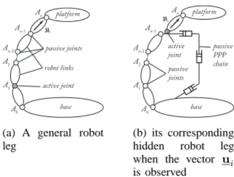
Let us consider a general leg for a parallel robot in which the direction uiof a segment is observed (Fig. 1(a) – in this figure, the last segment is considered observed, but the following explanations can be generalized to any segment located in the leg chain). In what follows, we only consider that we observe the leg direction ui, and not the leg edges in the image space, as the leg edges are only used as a measure of ui. So the problem is the same, except in the fact that we must consider the singularity of the mapping between the edges and ui, but this problem is well handled: these singularities appear when n1i and
n2i are colinear, i.e. the cylinders are at infinity [9]. In the general case, the unit vector ui can obviously be parameterized by two independent coordinates, that can be two angles, for example the angles α and β of Fig. III-A defined such thatcos α = x · v = y · w (where
v and w are defined such that z· v = z · w = 0) and
cos β = u · x. Thus α is the angle of the first rotation of
the link direction ui around z and β is the angle of the second rotation around v.
It is well known that a U joint is able to orientate a link aroud two orthogonal axes of rotation, such as z
ui platform base A0 A1 A2 An An-1 An-2 passive joints active joint robot links
(a) A general robot leg ui platform base A0 A1 A2 An An-1 An-2 passive joints active joint passive PPP chain (b) its corresponding
hidden robot leg
when the vector ui
is observed
Fig. 1. A general robot leg and its corresponding hidden robot leg
when the vector uiis observed
x y z ui : observed direction w α β v virtual cardan joint v .z=0 w.z=0
Fig. 2. Parameterization of a unit vector uiwith respect to a given frame x, y and z
and v. Thus U joints can be the virtual actuators with generalized coordinates α and β we are looking for. Of course, other solutions can exist, but U joints are the simplest ones.
If a U joint is the virtual actuator that makes the vector
ui move, it is obvious that: • if the value of u
i is fixed, the U joint coordinates
α and β must be constant, i.e. the actuator must be blocked,
• if the value of u
iis changing, the U joint coordinates
α and β must also vary.
As a result, to ensure the aforementioned properties for
α and β if ui is expressed in the base or camera frame
(but the problem is identical as the camera is considered fixed on the ground), vectors x, y and z of Fig. III-A must be the vectors defining the base or camera frame. Thus, in terms of properties for the virtual actuator, this implies that the first U joint axis must be constant w.r.t. the base frame, i.e. the U joint must be attached to a link
performing a translation w.r.t. the base frame3.
However, in most of the cases, the real leg architecture is not composed of U joints attached on links performing a translation w.r.t. the base frame. Thus, the architecture of the hidden robot leg must be modified w.r.t. the real leg such as depicted in Fig. 1(b). The U joint must be mounted on a passive kinematic chain composed of at most 3 orthogonal passive P joints that ensures that the link on which is it attached performs a translation w.r.t. the base frame. This passive chain is also linked to the segments before the observed links so that they do not change their kinematic properties in terms of motion. Note that:
3In the case where the camera is not mounted on the frame but on a moving link, the virtual U joint must be attached on a link performing a translation w.r.t. the considered moving link.
u A B C U joint R joint (a) A RU leg u PP chain A B C U joint mounted on the PP chain R joint
(b) Virtual{R–PP}–U leg
Planar parallelogram (Π) joint u A B C U joint mounted on the link BD R joint E D
(c) Virtual ΠU leg Fig. 3. A RU leg and two equivalent solutions for its hidden leg
• it is necessary to fix the PPP chain on the preceeding leg links because the information given by the vec-tors uiis not enough for rebuilding the full platform position and orientation: it is also necessary to get information on the location of the anchor point An−1 of the observed segment [9]. This information is kept through the use of the PPP chain fixed on the first segments;
• 3 P joints are only necessary if and only if the point
An−1describes a motion in the 3D space; if not, the number of P joints can be decreased: for example, in the case of the GS platform presented in [13], the U joint of the leg to control was located on the base, i.e. there was no need to add passive P joints to keep the orientation of its first axis constant; • when the vector u
i is constrained to move in a plane such as for planar legs, the virtual actuator becomes an R joint which must be mounted on the passive PPP chain (for the same reasons as mentioned previously).
For example, let us have a look at the RU leg with one actuated R joint followed by a U joint of Fig. 3(a). Using the previous approach, its virtual equivalent leg should be an {R–PP}–U leg (Fig. 3(b)), i.e. the U joint
able to orientate the vector ui is mounted on the top of a R–PP chain that can garantee that:
1) the link on which the U joint is attached performs a translation w.r.t. the base frame,
2) the point C (i.e. the centre of the U joint) evolves on a circle of radius lAB, like the real leg. It should be noticed that, in several cases for robots with a lower mobility (i.e. spatial robots with a number of dof less than 6, or planar robots with a number of dof less than 3), the last joint that links the leg to the platform should be changed so that, if the number of observed legs is inferior to the number of real legs, the hidden robot
keeps the same number of controlled dof.
It should also be mentioned that we have presented above the most general methodology that is possible to propose, but it is not the most elegant way to proceed. In many cases, a hidden robot leg architecture can be obtained such that less modifications w.r.t the real leg are achieved. For example, the R–PP chain of the hidden robot leg {R–PP}–U (Fig. 3(b)) could be equivalently
replaced by a planar parallelogram (Π) joint without
changing the aforementioned properties of the U virtual actuator (Fig. 3(c)), i.e. only one additional joint is added for obtaining the hidden robot leg (note that we consider that a Π joint, even if composed of several pairs, can be
seen as one single joint, as in [14]).
B. How to use the hidden robot models for analyzing the controllability of the servoed robots
The aim of this Section is to show how to use the hidden robots for answering points 1 to 4 enumerated in the introduction of the paper.
Point 1: the hidden robot model can be used to explain why the observed robot which is composed of n legs can be controlled using the observation of only m leg directions (m < n) arbitrarily chosen among its n legs, and can also help to choose the best set of legs to observe with respect to some given performance indices.
For answering this point, let us consider a general parallel robot composed of 6 legs (one actuator per leg) and having six dof. Using the approach proposed in Section III-A, each observed leg will lead to a modified virtual leg with at least one actuated U joint that has two degrees of actuation. For controlling 6 dof, only 6 degrees of actuations are necessary, i.e. three actuated U are enough. Thus, in a general case, only three legs have to be observed to fully control the platform dof.
Point 2: the hidden robot model can be used to prove that there does not always exist a full diffeomorphism between the Cartesian space and the leg direction space, but can also bring solutions for avoiding to converge to a non desired pose.
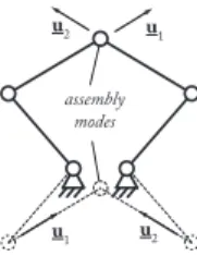
Here, the answer comes directly from the fact that the real controlled robot may have a hidden robot model with different geometric and kinematics properties. This means that the hidden robot may have assembly modes and singular configurations different from those of the real robot. If the initial and final robot configurations are not included in the same aspect (i.e. a workspace area that is singularity-free and bounded by singularities [2]), the robot won’t be able to converge to the desired pose, but to a pose that corresponds to another assembly mode that has the same leg directions as the desired final pose (see Fig. III-B).
Point 3: the hidden robot model simplifies the singularity analysis of the mapping between the leg direction space and the Cartesian space by reducing the problem to the singularity analysis of a new robot.
The interaction matrix MT involved in the controller gives the value of c˙u as a function of cτ
c. Thus, MT u1 u2 assembly modes u1 u2
Fig. 4. Two configurations of a five bar mechanism for which the
directions uiare identical (for i = 1, 2)
is the inverse Jacobian matrix of the hidden robot (and, consequently, MT+is the hidden robot Jacobian matrix). Except in the case of decoupled robots [19], [20], [21], the Jacobian matrices of parallel robots are not free of singularities.
Considering the input/output relations of a robot, three different kinds of singularity can be observed [22]4:
• the Type 1 singularities that appear when the robot Jacobian matrix is rank-deficient; in such configura-tions, any motion of the actuator that belongs to the kernel of the Jacobian matrix is not able to produce a motion of the platform,
• the Type 2 singularities that occur when the robot inverse Jacobian matrix is rank-deficient; in such configurations, any motion of the platform that be-longs to the kernel of the inverse Jacobian matrix is not able to produce a motion of the actuator. And, re-ciprocally, near these configurations, a small motion of the actuators lead to large platform displacements, i.e. the accuracy of the robot becomes very poor, • the Type 3 singularities that appear when both the
robot Jacobian and inverse Jacobian matrices are rank-deficient.
Thus,
• finding the condition for the rank-deficiency of MT is equivalent to find the Type 2 singularities of the hidden robot,
• finding the condition for the rank-deficiency of
MT+ is equivalent to find the Type 1 singularities of the hidden robot.
Point 4: the hidden robot model can be used to certify that the robot will not converge to local minima.
The robot could converge to local minima if the matrix
LT+ of (7) is rank deficient. A necessary and sufficient condition for the rank deficiency of this matrix is that the MT+ is rank deficient, i.e. the hidden robot model encounters a Type 1 singularity. As mentioned above, many tools have been developed by the mechanical design community for finding the singular configurations of robots and solutions can be provided to ensure that the hidden robot model does not meet any Type 1 singularity.
4There exist other types of singularities, such as the constraint singularities [23], but they are due to passive constraint degeneracy only, and are not involved in the mapping between the leg directions space and the robot controlled Cartesian coordinate space.
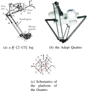
Ai Bi1 Ci1 ui Fixed base Bi2 Ci2 ui O Moving platform Prox. link Parallelogram Bi xi yi zi Ci P vi
(a) a R–{2–US} leg (b) the Adept Quattro
C4 C1 C2 C3 D1 D2 φ x y E4 E1 E2 E3 Cl (c) Schematics of the platform of the Quattro
Fig. 5. Example of leg and of robot of the Delta-like family
Ai Ci1 Fixed base Bi2 Ci2 ui Moving platform Spatial parallelogram Bi Ci vi Planar parallelogram Ai2 Ai1 Bi3 Bi4
(a) a Π–{2–UU} leg
Fixed base Articulated moving platform Pi Pj
(b) the hidden robot model for the Adept Quattro
Ai ui Moving platform Bi Ci ui Actuated U joint BiCi Si Ci : Vertex space of leg i Free motion of point Bi CiDi Bi3 Bi4 Di C iDi lAiBi
(c) vertex space of point Di
(projection of the Π–{2–UU}
leg in a vertical plane)
Fixed base Pi P j Uncontrolled platform motion
Ci: vertical slice of the
Bohemian Dome for a constant platform orientation Cj Articulated moving platform
(d) example of a Type 2 singularity for a 2–Π(2–UU) robot: the plat-form gets an uncontrollable trans-lation
Fig. 6. Example of leg and of hidden robot for the Delta-like family
For illustating this Section, let us present the fkp and singularity analysis of the hidden robot model of the Quattro with 4 dof (that can perform Schoenflies mo-tions), when controlled using leg direction observation. It must be mentionned that, in [15], the Quattro with rigid platform, i.e. with 3 translation dof was studied. However, the kinematics of the hidden robot for the version with 4 dof is completely different and is the object of this Section.
The Quattro is made of 4 R–{2–US} legs, thus its
equivalent hidden robot will be made of Π–{2–US}
or Π–{2–UU} legs. As such hidden robot legs have
2 degrees of actuation (the U joint is fully actuated), only two legs have to be observed for fully controlling the Quattro using leg direction observation. However in this case, if the hidden robot has a 2–Π–{2–US}
architecture, the platform will have two uncontrolled dof. This phenomenon disappears ifΠ–{2–UU} legs are used
in the hidden robot model (Fig. 6 – in this picture, the articulated platform is simplified for a clearer drawing, but has indeed the kinematic architecture presented in Fig. 5(c)).
Forward kinematics and assembly modes. Without loss
of generality, let us consider that we analyze the 2–Π– {2–UU} robot depicted at Fig. 6(a). Looking at the vertex
space of each leg when the active U joints are fixed, the points Ci and Di are carrying out a circle Ci of radius
lAiBi centred in Si (Fig. 6(c)).
The Quattro with 4 dof, and consequently its hidden robot model, has a particularity: its platform is passively articulated (Fig. 5(c)) so that its orientation with respect to the horizontal plan xOy stays constant, while it can have one degree of rotation around the z axis, i.e. point
D2can describe a circleCllocated in the horizontal plane, centred in D1 and with a radius lD1D2. For solving the forward kinematics, it is thus necessary to virtually cut the platform at point D2 and to compute the coupler surface of point D2when it belongs to leg 1. This coupler surface is the surface generated byClwhen it performs a circular translation alongC1. Such a surface is depicted in Fig. 7(a) and is called a Bohemian Dome [35].
A Bohemian Dome is a quartic surface, i.e. an alge-braic surface of degree 4. When it intersects the vertical planePlcontaining the circleC2(i.e. vertex space of the second leg), the obtained curve is a quartic curve (denoted atS1 – Fig.7(a)). And using the B´ezout theorem [36], it can be proven that, when the circle corresponding to the vertex space of leg 2 intersects this quartic curve, there can exist at most 8 intersection points, i.e. 8 assembly modes. Some examples of assembly modes for the 2–Π– {2–UU} robot are depicted in Figs. 7(b) and 7(c).
It should be noted that, when circles C1 and C2 are located in parallel planes, S1 degenerates into 1 or 2 circles. In this case, the maximal number of assembly modes decreases to 4. It must be mentioned here that, in usual controllers when only the encoder data is used, the number of assembly modes of the Quattro is equal to 8.
Singular configurations. For the 2–Π–{2–UU} robot,
Type 2 singularities appear when the planes Pi and Pj (whose normal vectors are equal to v⊥
i and v ⊥ j, resp.) are parallel. In such cases, the circle C2 is tangent to the Bohemian Dome at their intersection point and the robot gains one uncontrollable dof along this tangent (Fig. 6(d)).
C. Selection of the Controlled Legs
This Section has shown the importance of studying the intrinsic properties of the controller that are directly related to the choice of the stacked interaction matrices required for computing the control law. Depending on the chosen interaction matrices, i.e. on the choice of the observed legs, the geometry of the hidden robot models will vary, as well as its singularities and assembly modes. As singularities divide the workspace into distinct aspects [2], it is necessary to study the motion feasibility
circle C2 : vertex space of the 2nd leg coupler surface (Bohemian Dome) actuated U joints (on Π joints) u1 passive motions of the Π joints platform Pl S1 S1 D2 A1 B1 C1
(a) Coupler surface when leg 2 is discon-nected vertex space of the 2nd leg coupler surface actuated U joints (on Π joints) u1 u2 passive motions of the Π joints platform
(b) First set of possible assembly modes vertex space of the 2nd leg coupler surface actuated U joints (on Π joints) u1 u2 passive motions of the Π joints platform
(c) Second set of possible assem-bly modes
Fig. 7. Solutions of the fkp for a 2–Π–{2–UU} robot (in this example,
only 4 assembly modes exist)
by selecting a set of legs that can allow the robot displacement. Moreover, even if the motion is feasible, if the robot goes close to a singularity, the positioning error can considerably grow.
Therefore, it is necessary to find the best set of legs to observe in order to get the best performances of the robot w.r.t. a desired task. For the sake of compactness, the methodology for this will not be presented here, but the reader is referred to [15] for more information on this. In the next Section, all the presented theoretical results are validated through experiments on the Adept Quat-tro [32].
IV. CASESTUDY
In this Section, simulations and experiments are per-formed on the Adept Quattro presented in the previous Section. For the sake of compactness, the simulations are not included in this paper, only their experimental validations.
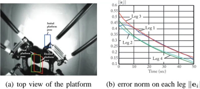
Testing the convergence of the robot to the desired pose
We replay now experimentally the convergence tests pre-sented in Section ??. The starting and desired final points are the same as previously. The results are presented in the Tables I to III and illustrated by the Figs. 8 to 10. It should be mentioned that, for cross-validating the results on those pictures, the plotted values of the error norms are computed using the values of the leg directions given by the Quattro controller.
Due to the presence of high measurement noise, the robot can of course not converge to the final desired pose.
Therefore, in these Tables, information on the tolerable maximal error on the pose attained attained in simulations is given. Please note that, due to the large value of the error on the measured angle, the model defined in Section ?? is no longer valuable and we have preferred to use a more refined non linearized model proposed in [38].
Initial platform pose Final platform pose Desired platform pose
(a) top view of the platform 0.05 0.1 0.15 0.2 0.25 0.3 0.35 0.4 0 10 20 30 40 50 Time (sec) ||ei|| Leg 3 Leg 1 Leg 4 Leg 2
(b) error norm on each legkeik
Fig. 8. Convergence of the robot when legs 1 and 4 are observed
(desired pose:{x = −0.2, y = 0, z = −0.56, φ = 0}).
TABLE I
RESULTS ON THE EXPERIMENTS CARRIED OUT FOR TESTING THE CONVERGENCE OF THE ROBOT WHEN LEGS1AND4ARE OBSERVED
(THE POSITIONS ARE IN METER,THE ANGLES IN RADIANS).
Desired final pose {x = −0.2, y = 0, z =
−0.56, φ = 0}
Final pose in simulation {x = −0.2, y = 0, z =
−0.91, φ = 0}
Tolerable position error 0.11 m
Tolerable orientation error 2.00 rad
Final pose in experiments {x = −0.11, y = 0.01, z =
−0.86, φ = −2.15}
Distance to the final pose in
simulation 0.10 m
Orient. err. w.r.t. the final pose
in simulation 2.15 rad
TABLE II
RESULTS ON THE EXPERIMENTS CARRIED OUT FOR TESTING THE CONVERGENCE OF THE ROBOT WHEN LEGS2AND3ARE OBSERVED
(THE POSITIONS ARE IN METER,THE ANGLES IN RADIANS).
Desired final pose {x = −0.2, y = 0, z =
−0.56, φ = 0}
Final pose in simulation {x = −0.2, y = 0, z =
−0.56, φ = 0}
Tolerable position error 0.23 m
Tolerable orientation error 1.23 rad
Final pose in experiments {x = −0.12, y = 0.05, z =
−0.55, φ = −0.90}
Distance to the final pose in
simulation 0.10 m
Orient. err. w.r.t. the final pose
in simulation 0.90 rad
All these experimental results match with the simulation results presented above and confirm the presence of the virtual robot hidden within the controller that must be studied in order to avoid the convergence problems due to inadequate stacking of interaction matrices.
Testing the presence of local minima
Initial platform pose
Final platform pose Desiredplatform
pose
(a) top view of the platform
0 10 20 30 40 50 0.1 0.15 0.2 0.25 0.3 0.35 0.4 0.45 0.5 0.55 0.6 Time (sec) ||ei|| Leg 3 Leg 1 Leg 4 Leg 2
(b) error norm on each legkeik
Fig. 9. Convergence of the robot when legs 2 and 3 are observed
(desired pose:{x = −0.2, y = 0, z = −0.56, φ = 0}). Initial platform pose Final platform pose Desired platform pose
(a) top view of the platform
2 4 6 8 10 0.01 0.02 0.03 0.04 0.05 0.06 0.07 0.08 0 Time (sec) ||ei|| Leg 3 Leg 1 Leg 4 Leg 2
(b) error norm on each legkeik Fig. 10. Convergence of the robot when all legs are observed (desired
pose:{x = 0.03, y = 0.03, z = −0.59, φ = 0}).
TABLE III
RESULTS ON THE EXPERIMENTS CARRIED OUT FOR TESTING THE CONVERGENCE OF THE ROBOT ALL LEGS ARE OBSERVED(THE
POSITIONS ARE IN METER,THE ANGLES IN RADIANS).
Desired final pose {x = 0.03, y = 0.03, z =
−0.59, φ = 0}
Final pose in simulation {x = 0.03, y = 0.03, z =
−0.65, φ = 0}
Tolerable position error 0.08 m
Tolerable orientation error 1.54 rad
Final pose in experiments {x = 0.05, y = 0.03, z =
−0.72, φ = 0.05}
Distance to the final pose in
simulation 0.07 m
Orient. err. w.r.t. the final pose
in simulation 0.05 rad
as the robot controller is designed with safeties that cannot be suppressed and that prevent going into singularities. However, as the presence of local minima that are located in the Type 1 singularities was demonstrated in simulations, we think that this numerical proof brings enough strength to our demonstration concerning this point.
Testing the importance of the selection of the observed legs on the robot accuracy
We replay now experimentally the accuracy tests pre-sented in Section ??. The starting and desired final points are the same as previously, as well as the observed legs. Each experiment is run five times and we present here the maximal values obtained on the position and orientation error. The results are shown in the Tables IV to V.
Once again, all these experimental results match with the simulation results presented above and confirm the necessity to carefully select the set of legs to observe in order to obtain the best accuracy possible. However,
TABLE IV
RESULTS ON THE EXPERIMENTS CARRIED OUT FOR TESTING THE ACCURACY OF THE ROBOT WHEN LEGS{2, 3}OR{2, 4}ARE
OBSERVED.
Desired final pose {x = −0.2m, y = 0.01m, z = −0.7m,
Legs {2, 3} {2, 4}
Position error 0.11 m 0.23 m
Orientation error 0.06 rad 0.68 rad
TABLE V
RESULTS ON THE EXPERIMENTS CARRIED OUT FOR TESTING THE ACCURACY OF THE ROBOT WHEN LEGS{1, 4}, {1, 3, 4}OR
{1, 2, 3, 4}ARE OBSERVED.
Desired final pose {x = 0.03m, y = 0.03m, z = −
Legs {1, 4} {1, 3, 4}
Position error 0.11 m 0.09 m
Orientation error 0.39 rad 0.31 rad
it must be recalled that, even if observing all the legs lead to a better accuracy, this result must not hide the fact that some convergence problems can still appear, as shown previously.
All these experiments validate the theory presented in Section III. The results show the validity of the approach and also its importance: stacking several interaction ma-trices to derive a control scheme without doing a deep analysis of the intrinsic properties of the controller is clearly not enough. For avoiding the singularity problem due to the mapping between the robot space and leg space, whatever the number of observed legs (as, even if all legs are observed, there may be singularities of the mapping), the hidden robot kinematics must be analyzed to avoid the convergence and inaccuracy problems.
V. CONCLUSIONS
This paper has presented a tool named the “Hidden robot concept” that is well addressed for analyzing the controllability of parallel robots in leg-observation-based visual servoing techniques. It has been shown that the mentioned visual servoing techniques involves the existence of a virtual robot model, hidden into the controller, that is different from the real controlled robot. Considering this hidden robot model allowed the finding of a minimal representation for the leg-observation-based control of the studied robots that is linked to a virtual hidden robot which is a tangible visualization of the mapping between the observation space and the real robot Cartesian space. It has been shown that the hidden robot model can be used to:
1) explain why the observed robot which is composed of n legs can be controlled using the observation of only m leg directions (m < n) arbitrarily chosen among its n legs,
2) prove that there does not always exist a full diffeo-morphism between the Cartesian space and the leg direction space,
3) simplify the singularity analysis of the mapping between the leg direction space and the Cartesian space by reducing the problem to the singularity analysis of a new robot,
4) certify that the robot will not converge to local minima, through the application of tools developed for the singularity analysis of robots.
A general way to find the hidden robot models corre-sponding to the real robot controlled via leg-observation-based visual servoing techniques has been shown and the hidden robot models of some well known classes of paral-lel robots have been studied. It has been proven that, using this concept, it is possible to demonstrate, using tools developed by the mechanical design community, that the robot can be controlled or not with the aforementioned visual servoing techniques.
Finally, experimental validations made on an Adept Quattro robot have demonstrated the validity of the theoretical developments.
Thus, the concept of hidden robot model, associated with mathematical tools developed by the mechanical design community, is a powerful tool able to analyze the intrinsic properties of some controllers developed by the visual servoing community. Moreover, this concept showed that in some visual servoing approaches, stacking several interaction matrices to derive a control scheme without doing a deep analysis of the intrinsic properties of the controller is clearly not enough. Further investigations are required.
ACKNOWLEDGEMENTS
This work was supported by the French ANR project ARROW (ANR-2011BS3-006-01), by the French ANR project EquipEx RobotEx (ANR-10-EQPX-44) and by the European Union Program “Comp´etitivit´e R´egionale et Emploi 2007–2013” (FEDER – R´egion Auvergne).
The authors would like to thank Michel Coste from the Institut de Recherche Math´ematique de Rennes (Uni-versity of Rennes, France) for his smart advices about the use of the B´ezout theorem and the definition of the Bohemian Dome.
REFERENCES
[1] T. Leinonen, “Terminology for the theory of machines and mech-anisms,” Mechanism and Machine Theory, vol. 26, 1991. [2] J. Merlet, Parallel Robots, 2nd ed. Springer, 2006.
[3] ——, 2012. [Online]. Available: www-sop.inria.fr/members/Jean-Pierre.Merlet/merlet.html
[4] B. Espiau, F. Chaumette, and P. Rives, “A new approach to visual servoing in robotics,” IEEE Transactions on Robotics and
Automation, vol. 8, no. 3, 1992.
[5] R. Horaud, F. Dornaika, and B. Espiau, “Visually guided ob-ject grasping,” IEEE Transactions on Robotics and Automation, vol. 14, no. 4, pp. 525–532, 1998.
[6] P. Martinet, J. Gallice, and D. Khadraoui, “Vision based control law using 3D visual features,” in Proceedings of the World
Au-tomation Congress, WAC96, Robotics and Manufacturing Systems,
vol. 3, Montpellier, France, May 1996, pp. 497–502.
[7] N. Andreff, A. Marchadier, and P. Martinet, “Vision-based control of a Gough-Stewart parallel mechanism using legs observation,” in Proceedings of the IEEE International Conference on Robotics
and Automation, ICRA’05, Barcelona, Spain, April 18-22 2005,
pp. 2546–2551.
[8] V. Gough and S. Whitehall, “Universal tyre test machine,” in
Proceedings of the FISITA 9th International Technical Congress,
May 1962, pp. 117–317.
[9] N. Andreff, T. Dallej, and P. Martinet, “Image-based visual servo-ing of gough-stewart parallel manipulators usservo-ing legs observation,”
International Journal of Robotics Research, vol. 26, no. 7, pp.
677–687, 2007.
[10] E. Ozgur, N. Andreff, and P. Martinet, “Dynamic control of the quattro robot by the leg edgels,” in Proceedings of the IEEE
International Conference on Robotics and Automation, ICRA11,
Shanghai, China, May 9-13 2011.
[11] N. Andreff and P. Martinet, “Vision-based kinematic modelling of some parallel manipulators for control purposes,” in Proceedings
of EuCoMeS, the First European Conference on Mechanism Science, Obergurgl, Austria, 2006.
[12] F. Chaumette, The Confluence of Vision and Control, ser. LNCIS. Springer-Verlag, 1998, no. 237, ch. Potential problems of stability and convergence in image-based and position-based visual servo-ing, pp. 66–78.
[13] S. Briot and P. Martinet, “Minimal representation for the control of Gough-Stewart platforms via leg observation considering a hidden robot model,” in Proceedings of the 2013 IEEE International
Conference on Robotics and Automation (ICRA 2013), Karlsruhe,
Germany, May, 6-10 2013.
[14] S. Caro, W. Khan, D. Pasini, and J. Angeles, “The rule-based conceptual design of the architecture of serial schonflies-motion generators,” Mechanism and Machine Theory, vol. 45, no. 2, pp. 251–260, 2010.
[15] V. Rosenzveig, S. Briot, and P. Martinet, “Minimal representation for the control of the Adept Quattro with rigid platform via leg observation considering a hidden robot model,” in Proceedings of
the IEEE/RSJ International Conference on Intelligent Robots and Systems (IROS 2013), Tokyo Big Sight, Japan, 2013.
[16] N. Andreff, B. Espiau, and R. Horaud, “Visual servoing from lines,” International Journal of Robotics Research, vol. 21, no. 8, pp. 679–700, 2002.
[17] J. Pl¨ucker, “On a new geometry of space,” Philosophical
Trans-actions of the Royal Society of London, vol. 155, pp. 725–791,
1865.
[18] F. Chaumette, La commande des robots manipulateurs. Herm`es,
2002.
[19] M. Carricato and V. Parenti-Castelli, “Singularity-free fully-isotropic translational parallel manipulators,” International
Jour-nal of Robotics Research, vol. 21, no. 2, pp. 161–174, 2002.
[20] X. Kong and C. Gosselin, “A class of 3-dof translational parallel manipulators with linear input-output equations,” in Proceedings
of the Workshop on Fundamental Issues and Future Research Directions for Parallel Mechanisms and Manipulators, Qu´ebec
City, QC, Canada, October 2002, pp. 3–4.
[21] G. Gogu, “Structural synthesis of fully-isotropic translational parallel robots via theory of linear transformations,” European
Journal of Mechanics. A/Solids, vol. 23, no. 6, pp. 1021–1039,
2004.
[22] C. Gosselin and J. Angeles, “Singularity analysis of closed-loop kinematic chains,” IEEE Transactions on Robotics and
Automa-tion, vol. 6, no. 3, pp. 281–290, 1990.
[23] D. Zlatanov, I. Bonev, and C. Gosselin, “Constraint singularities of parallel mechanisms,” in Proceedings of the IEEE International
Conference on Robotics and Automation (ICRA 2002), May 2002.
[24] I. Bonev, D. Zlatanov, and C. Gosselin, “Singularity analysis of 3-dof planar parallel mechanisms via screw theory,” ASME Journal
of Mechanical Design, vol. 125, no. 3, pp. 573–581, 2003.
[25] P. Ben-Horin and M. Shoham, “Singularity analysis of a class of parallel robots based on grassmanncayley algebra,” Mechanism
and Machine Theory, vol. 41, no. 8, pp. 958–970, August 2006.
[26] S. Caro, G. Moroz, T. Gayral, D. Chablat, and C. Chen, “Singu-larity analysis of a six-dof parallel manipulator using grassmann-cayley algebra and grobner bases,” in Proceedings of the
Sym-posium on Brain, Body and Machine, Montreal, QC, Canada,
November 10-12 2010.
[27] R. Clavel, “Device for the movement and positioning of an element in space,” US Patent 4 976 582, December 11, 1990. [28] S. Krut, O. Company, M. Benoit, H. Ota, and F. Pierrot, “I4: A
new parallel mechanism for Scara motions,” in Proceedings of
the 2003 International Conference on Robotics and Automation (ICRA 2013), 2003.
[29] L. Tsai and S. Joshi, “Comparison study of architectures of four 3 degree-of-freedom translational parallel manipulators,” in
Proceedings of the IEEE International Conference on Robotics and Automation (ICRA 2001), 2001.
[30] F. Pierrot, M. Uchiyama, P. Dauchez, and A. Fournier, “A new design of a 6-dof parallel robot,” Proceedings of the 23rd
Inter-national Symposium on Industrial Robots. Jounrla of Robotics and Mechatronics, pp. 308–315, 1990.
[31] M. Honegger, A. Codourey, and E. Burdet, “Adaptive control of the Hexaglide, a 6 dof parallel manipulator,” in Proceedings of
the IEEE International Conference on Robotics and Automation (ICRA 1997), 1997.
[32] V. Nabat, M. de la O Rodriguez, O. Company, S. Krut, and F. Pier-rot, “Par4: very high speed parallel robot for pick-and-place,” in
Proceedings of the 2005 IEEE/RSJ International Conference on Intelligent Robots and Systems (IROS 2005)., 2005.
[33] D. Chablat and P. Wenger, “Architecture optimization of a 3-dof parallel mechanism for machining applications, the Orthoglide,”
IEEE Transactions on Robotics and Automation, vol. 19, no. 3,
pp. 403–410, 2003.
[34] O. Company and F. Pierrot, “Modelling and preliminary design is-sues of a 3-axis parallel machine-tool,” Mechanisms and Machine
Theory, vol. 37, pp. 1325–1345, 2002.
[35] M. Tale Masouleh, C. Gosselin, M. Husty, and D. Walter, “For-ward kinematic problem of 5-RPUR parallel mechanisms (3T2R) with identical limb structures,” Mechanism and Machine Theory, vol. 46, pp. 945–959, 2011.
[36] E. B´ezout, Recherches sur le degr´e des ´equations r´esultantes de
l’´evanouissement des inconnues. Histoire de l’Acad´emie Royale des Sciences, 1764.
[37] J. Merlet, “Jacobian, manipulability, condition number, and accu-racy of parallel robots,” ASME Transactions Journal of
Mechan-ical Design, vol. 128, no. 1, pp. 199–206, 2006.
[38] S. Briot and I. Bonev, “Accuracy analysis of 3T1R fully-parallel robots,” Mechanism and Machine Theory, vol. 45, no. 5, pp. 695– 706, 2010.
[39] A. Pashkevich, D. Chablat, and P. Wenger, “Stiffness analysis of overconstrained parallel manipulators,” Mechanism and Machine
Theory, vol. 44, no. 5, pp. 966–982, 2009.
[40] N. Binaud, P. Cardou, S. Caro, and P. Wenger, “The kinematic sen-sitivity of robotic manipulators to joint clearances,” in Proceedings
of ASME Design Engineering Technical Conferences, Montreal,
QC, Canada, August 15-18 2010.
[41] S. Briot and V. Arakelian, “Optimal force generation of parallel manipulators for passing through the singular positions,”
Interna-tional Journal of Robotics Research, vol. 27, no. 8, pp. 967–983,
2008.
[42] D. Chablat, G. Moroz, and P. Wenger, “Uniqueness domains and non singular assembly mode changing trajectories,” in
Proceed-ings of the 2011 IEEE International Conference on Robotics and Automation (ICRA 2011), Shanghai, China, 2011.
[43] SiRoPa Toolbox. [Online]. Available: