Influence du paysage sur une communauté de Strigidés en tenant compte de la probabilité de détection

INFLUENCE DU PAYSAGE SUR UNE COMMUNAUTE DE STRIGIDES EN TENANT COMPTE DE LA PROBABILITE DE DETECTION

Par

Genevieve Perreault

Memoire presente au Departement de biologie en vue de l'obtention du grade de maitre es Sciences (MSc.)

FACULTE DES SCIENCES UNIVERSITE DE SHERBROOKE

1*1

Your file Votre reference ISBN: 978-0-494-61466-2 Our file Notre reference ISBN: 978-0-494-61466-2

NOTICE: AVIS:

The author has granted a

non-exclusive license allowing Library and Archives Canada to reproduce, publish, archive, preserve, conserve, communicate to the public by

telecommunication or on the Internet, loan, distribute and sell theses

worldwide, for commercial or non-commercial purposes, in microform, paper, electronic and/or any other formats.

L'auteur a accorde une licence non exclusive permettant a la Bibliotheque et Archives Canada de reproduce, publier, archiver, sauvegarder, conserver, transmettre au public par telecommunication ou par I'lnternet, preter, distribuer et vendre des theses partout dans le monde, a des fins commerciales ou autres, sur support microforme, papier, electronique et/ou autres formats.

The author retains copyright ownership and moral rights in this thesis. Neither the thesis nor substantial extracts from it may be printed or otherwise reproduced without the author's permission.

L'auteur conserve la propriete du droit d'auteur et des droits moraux qui protege cette these. Ni la these ni des extraits substantiels de celle-ci ne doivent etre imprimes ou autrement

reproduits sans son autorisation.

In compliance with the Canadian Privacy Act some supporting forms may have been removed from this thesis.

While these forms may be included in the document page count, their removal does not represent any loss of content from the thesis.

Conformement a la loi canadienne sur la protection de la vie privee, quelques

formulaires secondares ont ete enleves de cette these.

Bien que ces formulaires aient inclus dans la pagination, il n'y aura aucun contenu manquant.

1+1

Canada

Le 15 Janvier 2010

lejury a accepte le memoire de Madame Genevieve Perreault dans sa version finale.

Membres du jury

Professeur Marc Belisle Directeur de recherche Departement de biologie

Professeur Marco Festa-Bianchet Membre

Departement de biologie

Professeur Dany Garant President rapporteur Departement de biologie

SOMMAIRE

Plusieurs etudes ont tente de decrire 1'influence de la structure du paysage sur la distribution des Strigides. Certaines ont meme essaye de quantifier l'impact de la perte et de la fragmentation d'habitas sur ces oiseaux. Cependant, la majorite de ces etudes n'ont pas tenu compte de la probabilite de detection imparfaite lors de l'echantillonnage, ni considere que les interactions entre les differentes especes pouvaient interferer avec cette distribution. Dans cette etude, je mesure l'influence de la structure du paysage sur la distribution du Grand-due d'Amerique (Bubo virginianus), de la Chouette rayee (Strix varia) et de la Petite Nyctale (Aegolius acadicus) parmi 112 sites repartis a travers un large gradient « foret-agriculture » dans le Sud du Quebec. Je mesure egalement l'impact des interactions interspecifiques sur cette distribution. Afin de determiner si la sequence d'enregistrements utilisee lors des recensements de Strigides affecte la detection de ceux-ci, je compare les probabilites de detections obtenues dans les recensements ou le chant d'une seule espece est diffuse avec celles des recensements ou le chant d'une espece est diffuse suite a celui d'un competiteur ou d'un predateur.- Finalement, j'effectue deux versions des analyses afin de comparer les resultats obtenus a l'aide de simples regressions logistiques a ceux obtenus lorsque la probabilite de detection est consideree. Mes resultats indiquent que la probabilite d'occurrence du Grand-due d'Amerique ne semble pas etre affectee par la composition du paysage et que sa probabilite de detection n'est pas influencee par la sequence d'enregistrements utilisee lors de l'inventaire. Par ailleurs, la probabilite d'occurrence de la Chouette rayee et de la Petite Nyctale augmente avec le couvert forestier et, par le fait meme, diminue avec le couvert agricole. La presence d'un predateur ou d'un competiteur dans le paysage ne semble pas influencer la distribution des Strigides. Cependant, les chants du Grand-due d'Amerique diminuent la detectabilite de la Chouette rayee. Bien que les chants du Grand-due ne semblent pas affecter la detectabilite de la Petite Nyctale en tant que telle, la probabilite de detection de celle-ci est toutefois moins elevee lorsque le chant du Grand-due d'Amerique est diffuse avant son propre chant. Finalement, j'obtiens des resultats differents en considerant la probabilite de detection ou non. Plus precisement, certaines variables avaient un effet significatif dans une seule version des analyses, ou encore la magnitude de 1'effet etait differente selon le type d'analyse utilise. Ceci laisse sous entendre que plusieurs parametres peuvent influencer la probabilite de detection des Strigides et qu'elle devrait toujours etre consideree dans les recensements de rapaces nocturnes.

REMERCIEMENTS

Je tiens a remercier mon directeur de recherche, Marc Belisle, qui a accepte de superviser ce projet qui debordait de ses champs d'etudes habituels. La liberie qu'il m'a offerte dans la realisation de ce projet a ete pour moi une grande source de motivation. Ses connaissances en statistiques ont egalement ete une veritable mine d'or pour une etudiante qui partait de loin dans ce domaine. « Entre toi, pis moi, pis la boite a pain », un gros merci!

Je remercie egalement mes deux compagnons de route, Benoit Gendreau et Marie-Claude Martin, qui ont accepte d'affronter la solitude, l'hiver et la nuit pour effectuer avec moi les 2240 recensements de rapaces nocturnes necessaires a cette etude. Sans vous, je n'y serais jamais arrivee.

Merci a Dairy Garant et Marco Festa-Bianchet d'avoir partage leur point de vue sur ce projet. Merci a Marc Mazerolle pour son aide avec le logiciel PRESENCE, et a Caroline Girard et Gabriel Diab pour leur expertise en geomatique. Merci a Benoit Lapointe pour son aide dans les preparatifs du terrain et son incomparable disponibilite.

Finalement, merci a tous les membres du labp avec qui j'ai partage un bout de chemin : Arnaud, Audrey, Claudie, Francois, Louis, Ludovic, Marie-Claude, Stephane et Yanick. Merci pour le support moral, les encouragements, les echanges de services et les moments d'angoisses existentielles. Cette maitrise n'aurait pas ete aussi agreable sans vous!

Ce projet a ete realise grace au support financier de la Chaire de recherche du Canada en ecologie spatiale et en ecologie du paysage, la Fondation canadienne pour 1'innovation, les Fonds quebecois de la recherche sur la nature et les technologies, le Conseil de recherches en sciences naturelles et en genie du Canada, et l'Universite de Sherbrooke.

TABLE DES MATIERES

SOMMAIRE ii REMERCIEMENTS iii

TABLE DES MATIERES iv LISTE DES TABLEAUX vii LISTE DES FIGURES viii LISTE DES ANNEXES ix INTRODUCTION GENERALE .. 1

Laperte et la fragmentation des habitats 1

L'interet d'etudier les Strigides 3 Interactions entre especes. 4 Le recensement des Strigides , 5

La probability de detection. 7 Les objectifs de cette etude. ' 9

CHAPITRE1 10 Mise en contexte 10 Abstract 11 Introduction 12 Methods 14 Model species 14 Great Horned Owl (GHOW) 15

Barred Owl (BDOW) 15 Northern Saw-whet Owl (NSWO) 16

Study area 16 Sampling design 18

Playbacks 18 Owl surveys 19 Data collection 20

Landscape characterization. 21

Statistical analyses 22 Assumptions 22 Models 23 Model selection and multi-model inference 26

Logistic regressions 26

Results 26 Effects of covariates on detection 28

GHOW2008 28 BDOW 2007-2008 29 NSWO2007 29 Effects of covariates on occupancy 31

GHOW2008 31 BDOW 2007-2008 31 NSWO2007 , 32 Logistic regressions 33 Discussion 34 Detection :. 35 Broadcast 35 Date 37 Hour 38 Other factors 38 Occupancy. 39 GHOW. 39 BDOW and NSWO 39

Additional variables of interest 42 Accounting for imperfect detection 43

Conclusion 44 Acknowledgements 45

Appendix 2 47 Literature cited 48 CONCLUSION GENERALE 56

LISTE DES TABLEAUX

CHAPITRE 1

1. Explanatory variables used to assess the occurrence and detection probability of Great Horned (GHOW), Barred (BDOW) and Northern Saw-whet (NSWO) Owl in 2007 and 2008 within agricultural landscapes of southern Quebec,

Canada 24

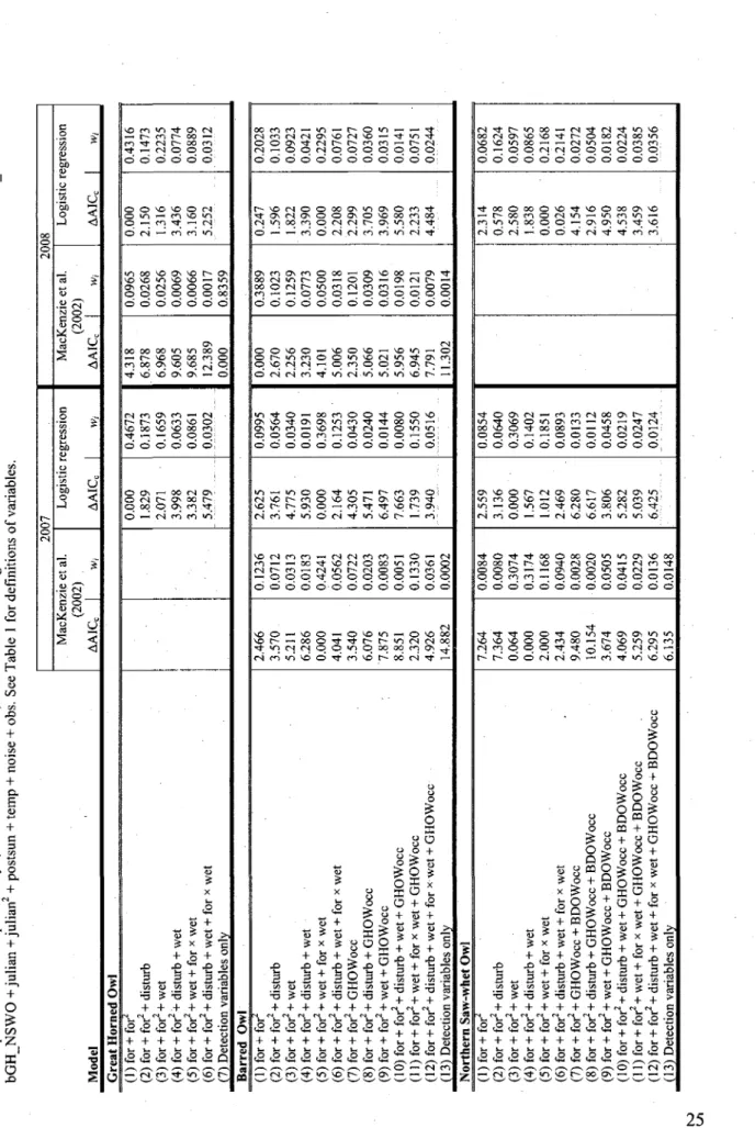
2. Model selection for owl occupancy in agricultural landscapes of southern Quebec, Canada, using two different types of analyses. Models accounting for imperfect detection probability (MacKenzie et al. 2002) shared the following additional detection covariates: bBDOW + bNSWO + bGHBDOW + bGHNSWO + Julian + Julian2 + postsun + temp + noise + obs. See Table 1 for

definitions of variables 25

3. Detection and occurrence probabilities of owls in southern Quebec as estimated following MacKenzie et al. (2002). Naive occupancy estimates (i.e., not corrected for imperfect detection) are also presented. These estimates were obtained under average conditions (Appendices 1 and 2) and using conspecific

calls in an average landscape without predator or competitor. 27

4. Effects of detection probability covariates obtained following MacKenzie et al. (2002) and subjected to multi-model inference. Regression coefficients (9) are shown with their unconditional standard errors (SE) and 95% confidence intervals. Note that all values are expressed in logit. See Table 1 for definitions

of variables and Table 2 for the set of models 27

5. Effects of occupancy covariates obtained when accounting for imperfect detection (MacKenzie et al. 2002) or through logistic regressions and subjected to multi-model inference. Regression coefficients (9) are shown with their unconditional standard errors (SE) and 95% confidence intervals. Note that all values are expressed in logit. See Table 1 for definitions of variables and Table

LISTE DES FIGURES

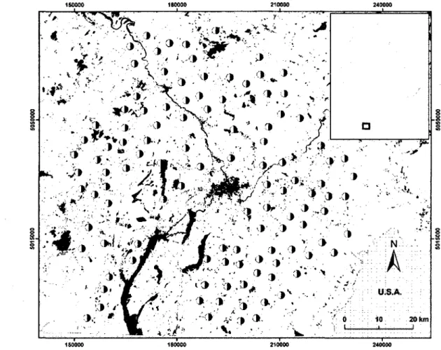
1. Distribution of the 112 sites surveyed for owls in 2007-2008 in southern Quebec, Canada. Black and white circles indicate site locations. Land cover types include forest (white), disturbed forest (light gray), agriculture (mid-tone

gray), urban (dark gray), and water (black). Coordinate units are UTM 17

2. Relationship between agriculture and forest covers within 1km and 2km radii

for the 112 survey sites in southern Quebec, Canada (Fig. 1) 18

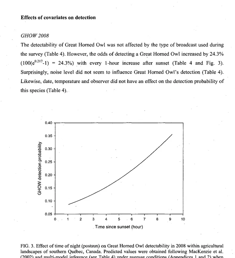
3. Effect of time of night (postsun) on Great Horned Owl detectability in 2008 within agricultural landscapes of southern Quebec, Canada. Predicted values were obtained following MacKenzie et al. (2002) and multi-model inference , (see Table 4) under average conditions (Appendices 1 and 2) when using

conspecific calls in an average landscape without predator or competitor 28

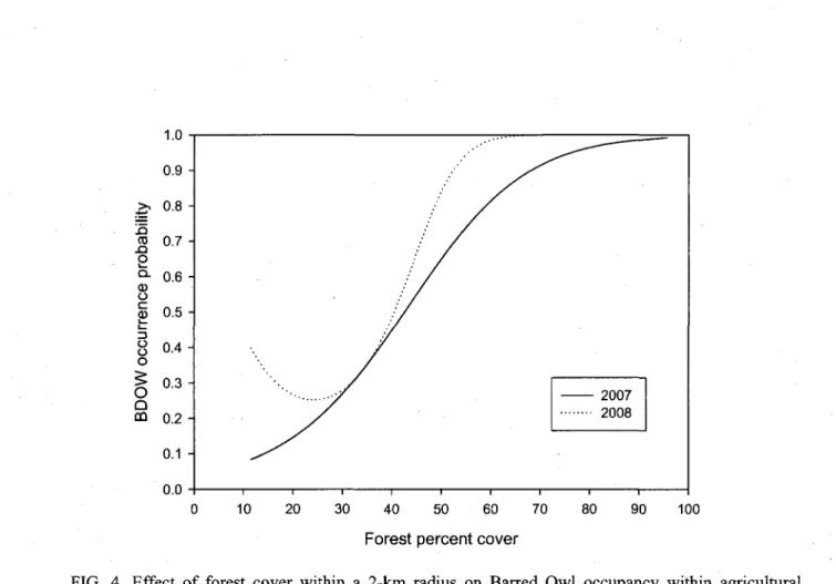
4. Effect of forest cover within a 2km radius on Barred Owl occupancy within agricultural landscapes of southern Quebec, Canada. Predicted values were obtained following MacKenzie et al. (2002) and multi-model inference (see Table 5) under average conditions (Appendices 1 and 2) when using conspecific calls in an average landscape without predator or competitor. Note that 2008 is illustrated here to show constancy of results although forest cover did not

significantly influence occupancy for that year 32

5. Effect of forest cover within a 1km radius on Northern Saw-whet Owl occupancy for various wetland percent covers in 2007 within agricultural landscapes of southern Quebec, Canada. Predicted values were obtained following MacKenzie et al. (2002) and multi-model inference (see Table 5) under average conditions (Appendices 1 and 2) when using conspecific calls in an average landscape without predator or competitor. Note that wetland cover includes both the water (rivers, lakes) riparian habitats and the actual wetlands

LISTE DES ANNEXES

1. Average (± SD) conditions met during owl surveys conducted in agricultural

landscapes of southern Quebec, Canada 46

2. Average (+ SD) land covers for the 112 sites surveyed for owls in southern

INTRODUCTION GENERALE

La foresterie, l'agriculture et 1'urbanisation sont considerees comme les principales responsables de la perte et de la fragmentation des habitats naturels qui ont mene au declin de nombreuses populations animales (Lehtinen et al.,1999; Carlson, 2000; Schmiegelow et Monkkonen, 2002; Tscharntke et al., 2005). De plus, 1'intensification des pratiques forestieres et agricoles ont favorise une homogeneisation du paysage qui exacerbe les problemes causes par la perte et la fragmentation des habitats (Imbeau et al., 2001; Belanger et Grenier, 2002; McCracken et Tallowin, 2004; Tscharntke et al., 2005). En plus de transformer la composition et la configuration du paysage, la perte et la fragmentation des habitats modifient la distribution et l'abondance des ressources disponibles (Redpath, 1995; Fahrig, 2003). Or, chaque espece s'adapte differemment a ces changements, certaines ayant plus de facilite que d'autres (Deutschman et al., 1993; McKinney et Lockwood, 1999; Devictor et al., 2008). A titre d'exemple, en plus d'etre influences par les caracteristiques du paysage, la distribution des Strigides peut etre influencee par leurs interactions avec d'autres rapaces nocturnes (Hakkarainen et Korpimaki, 1996; Vrezec et Tome, 2004a, b). Pourtant, la majorite des etudes sur les Strigides font abstraction de ces interactions. De plus, les interactions interspecifiques pourraient influencer la detectabilite des Strigides lors des recensements et causer des biais lors de 1'estimation de parametres (Kelly et al., 2003; Olson et al., 2005; Crozier et al., 2006). Cependant, les programmes charges de faire le suivi des rapaces nocturnes ne tiennent pas compte des ces interactions et ne sont pas corriges pour une probabilite de detection imparfaite. Ce memoire portera sur la probabilite d'occurrence et de detection de trois especes de Strigides au Quebec, tout en considerant l'impact possible des interactions interspecifiques.

La perte et la fragmentation des habitats

Les effets de la perte et de la fragmentation des habitats sur les populations animales ont fait l'objet d'une plethore d'etudes depuis 1970 (e.g., Andren, 1994; Bender et al., 1998; Fahrig, 2003). Par exemple, il a ete demontre que la plupart des especes ont besoin d'une quantite

minimale d'habitat dans le paysage afin de pouvoir survivre (Andren, 1994; Fahrig, 2003). C'est le cas, entre autres, du Pic a dos blanc (Dendrocopos leucotos) qui requiert au moins 9-17% de foret decidue mature dans le paysage pour maintenir une population viable (Carlson, 2000). Par ailleurs, Belisle et al. (2001) ont demontre que les habitats fragmented contraignent les mouvements d'oiseaux forestiers comme la Paruline bleue (Dendroica caerulescens), la Paruline couronnee (Seiurus aurocapilla) et la Mesange a tete noire (Poecile atricapillus). Finalement, Hinsley (2000) a montre que la fragmentation augmente les couts de deplacement de la Mesange charbonniere (Parus major).

Parmi les nombreuses etudes effectuees sur la perte et la fragmentation d'habitat, la terminologie n'a pas toujours ete respectee et ces deux termes ont ete utilises a toutes les sauces. Comme son nom l'indique, la perte d'habitat est caracterisee par une diminution de la quantite d'habitat de bonne qualite dans le paysage. La perte d'habitat associee a une espece donnee a done toujours un impact negatif sur cette derniere (Fahrig, 2003). Pour sa part, la fragmentation a souvent ete associee, a tort, a une certaine perte d'habitat. Pourtant, la fragmentation n'est que la division d'une ou de plusieurs parcelles d'habitat dans le paysage, sans qu'il n'y ait de perte sensu stricto (Fahrig, 2003). II est important de noter que la perte et la fragmentation des habitats contribuent a la creation d'autres habitats et par consequent peuvent etre favorables a certaines especes (Bender et al., 1998; Fahrig, 2003). Par exemple, la fragmentation peut etre benefique pour une espece associee aux bordures forestieres ou a des jeunes stades de succession forestiere puisqu'elle augmente la quantite de ces types d'habitats dans le paysage (Andren, 1994; Fahrig, 2003; Imbeau et al., 2003). II demeure que la creation de bordures n'est avantageuse que pour un nombre restreint d'especes alors qu'elle penalise la majorite des communautes forestieres (Yahner, 1988; Bosakowski et Smith, 1997).

En plus d'augmenter la quantite de lisieres dans le paysage, la fragmentation a pour effet d'accroitre le nombre et l'isolement des parcelles d'habitat, de reduire la taille de celles-ci, et d'augmenter la quantite de nouveaux habitats (Andren, 1994). II semble que les especes generalistes s'adaptent plus facilement a ces changements que les specialistes (McKinney et Lockwood, 1999; Millan de la Pena et al., 2003; Marvier et al., 2004), favorisant ainsi

l'expansion des generalistes dans le paysage au detriment des especes specialistes (Bosakowski et Smith, 1997; McKinney et Lockwood, 1999; Millan de la Pena et al., 2003; Marvier et al., 2004). Ainsi, que le changement soit cause par la perte ou la fragmentation des habitats, il aura probablement un impact sur la distribution des especes dans le paysage.

L'interet d'etudier les Strigides

Etant donne leur nature cryptique et le fait qu'ils soient pour la plupart nocturnes, les Strigides sont parmi les oiseaux les moins connus. En effet, meme les inventaires d'oiseaux a grand deploiement, tels que les atlas des oiseaux nicheurs (e.g., Gauthier et Aubry, 1995), le

Breeding Bird Survey (Link et Sauer, 1998), ou le recensement des oiseaux de Noel (National

Audubon Society, 2002), ne procurent que tres peu d'information sur les Strigides puisque ces inventaires sont habituellement realises pendant le jour et a l'exterieur de leur periode de reproduction, periode ou leur detectabilite est plus elevee (Takats et al., 2001).

Pourtant, etant des predateurs de hauts niveaux trophiques, les Strigides jouent un role fondamental dans les processus ecologiques (Molles, 1999). Comme la plupart des oiseaux de proie, ils sont sensibles aux perturbations anthropiques et a la presence de polluants dans l'environnement (Bosakowski et Smith, 1997; Houston et al., 1998; Mazur et James, 2000; Johnsgard, 2002). II est done possible de les utiliser comme des « barometres » pour mesurer la qualite et la sante d'un habitat. De plus, certaines especes de Strigides, comme la Chouette rayee (Strix varia), sont considerees comme des especes indicatrices ou parapluie (Rubino et Hess, 2003; Olsen et al., 2006). Une espece indicatrice est fortement associee a un habitat particulier et represente la qualite de celui-ci (Niemi et al., 1997). En plus d'etre indicatrice, une espece parapluie possede habituellement un large domaine vital dans lequel se trouvent plusieurs autres especes associees (Roberge et Angelstam, 2004). Ainsi, definir la situation d'une espece parapluie dans un milieu permet 1'evaluation de la situation de plusieurs autres especes. Par le fait meme, en promulguant la conservation d'une espece parapluie, la conservation des especes associees devrait egalement etre favorisee (Roberge et Angelstam, 2004).

Interactions entre especes

Plusieurs etudes ont tente de quantifier 1'influence de la structure du paysage sur la distribution des Strigides dans l'espace (e.g., Folliard et al., 2000; Penteriani et al., 2004). Cependant, nulle espece ne se retrouve completement isolee des autres. II est done primordial de considerer l'impact que les interactions entre especes peuvent avoir sur cette distribution.

La competition et la predation contribuent a controler la densite et la distribution d'une population (Molles, 1999). Lorsque le predateur se nourrit d'une proie, il diminue inevitablement le nombre d'individu de cette population. Cependant, l'effet de la competition est plus complexe du fait qu'elle peut etre intraspecifique ou interspecifique (e.g., Savard, 1982; Essington et al., 2000; Harwood et al., 2002). Elle se produit lorsque deux ou plusieurs individus utilisent les memes ressources, par exemple, en ayant une diete similaire, en habitant le meme type d'habitat, ou en recherchant les memes sites de nidifications (Molles, 1999). Ainsi, les ressources alimentaires semblent etre une cause de competition pour le Garrot d'Islande {Bucephala islandica) et le Petit Garrot (B. albeola; Savard, 1982), alors que le Saumon de l'Atlantique (Salmo salar) et la Truite brune (S. trutta) se disputent les refuges disponibles dans le lit d'un cours d'eau (Harwood et al., 2002). Dans les deux cas, cette competition se produit autant entre individus de la meme espece qu'entre individus d'especes differentes. Chez les rapaces, la competition interspecifique se manifeste plus frequemment entre des especes de taille similaires (Hakkarainen et Korpimaki, 1996).

La competition comporte des couts non negligeables pour l'individu qui la subit. Entre autres, elle diminue les chances de survie et le succes reproducteur des competiteurs chez plusieurs especes comme le Gobemouche a collier {Ficedula albicollis', Gustafsson, 1987), le Campagnol roussatre (Clethrionomys glareolus; Eccard et Ylonen, 2002), ou le Saumon du Pacifique (Oncorhynchus sp.; Essington et al., 2000). Ainsi, deux especes competitrices auront communement recours a une segregation spatiale ou temporelle afin d'eviter ces effets nefastes. Par exemple, les rapaces peuvent modifier leur niche ou leur horaire de chasse dans le but de diminuer le chevauchement des ressources utilisees et les rencontres agressives entre

competiteurs (Hakkarainen et Korpimaki, 1996; Vrezec et Tome, 2004ab). Habituellement, le competiteur dominant parviendra eventuellement a exclure 1'autre espece (Vrezec et Tome, 2004ab). Generalement, la taille est un facteur determinant dans la selection d'habitat des Strigides. En effet, l'espece de plus grande taille selectionnera un habitat optimal alors que la seconde se contentera d'un habitat alternatif (Hakkarainen et Korpimaki, 1996; Vrezec et Tome, 2004b). De plus, le Strigide dominant peut pratiquer la predation sur le plus petit competiteur. Comme l'ont souligne Bluhm et Ward (1979), lorsqu'un rapace se nourrit d'un rapace de plus petite taille, il obtient non seulement la nourriture dont il a besoin, mais il elimine egalement un competiteur potentiel.

Les interactions entre les differentes especes de Strigides peuvent done influencer l'abondance et la distribution de ceux-ci dans le paysage. De meme, les interactions entre especes pourraient egalement avoir un impact sur la detectabilite des Strigides. En effet, un individu ayant entendu son competiteur ou son predateur pourrait etre moins enclin a chanter afin d'eviter une agression ou la predation (Kelly et al., 2003; Olson et al., 2005; Crozier et al., 2006). De plus, la densite de la population semble affecter l'activite vocale des Strigides (Penteriani et al., 2002). Chanter pour defendre son territoire comporte certains couts puisque, en plus de reveler sa presence aux predateurs, le temps investi au chant est soustrait au temps disponible pour d'autres activites comme chasser ou se reproduire. Or, Penteriani et al. (2002) ont observe que le Grand-due d'Europe {Bubo bubo) investissait moins d'energie pour chanter lorsque les voisins etaient inexistants ou lorsqu'ils etaient eloignes. Ainsi, dans une population ou la densite est faible, la necessite de chanter afin de defendre son territoire doit etre moins frequente.

Le recensement des Strigides

Les Strigides sont difficiles a recenser puisqu'ils sont nocturnes et qu'ils possedent de larges territoires a l'interieur desquels ils peuvent se deplacer rapidement (Fuller et Mosher, 1981; Johnsgard, 2002). Plusieurs techniques d'inventaire ont deja ete utilisees comme les points d'ecoute en bordure des routes, les recensements avec lampe de poche (spotlighting), les

transects (walking line-transect) et les recensements en voiture (driving survey; Conway et Simon, 2003; Condon et al., 2005). Cependant, la methode la plus souvent utilisee est le point d'ecoute avec repasse de chant (Takats et al., 2001). Cette methode se base sur le fait que les Strigides defendent leur territoire par le chant. La technique consiste a diffuser des enregistrements de chants de Strigides afin d'inciter les individus presents a repondre a l'appel (Takats et al., 2001). Le point d'ecoute avec repasse de chant est done une methode qui s'avere tres utile aupres d'especes difficiles a recenser visuellement. De plus, cette technique est tres efficace comparativement aux autres methodes de recensement puisqu'elle permet de detecter un plus grand nombre d'individus par unite de temps (Mosher et al., 1990).

Depuis plusieurs annees, des suivis de rapaces nocturnes sont effectues a l'aide de points d'ecoute avec repasse de chant un peu partout en Amerique du Nord (Takats et al., 2001; Balej, 2006; Etudes d'Oiseaux Canada, 2008). Ces recensements sont generalement realises par des ornithologues amateurs benevoles parcourant des routes preetablies par les organisateurs. La plupart du temps, chaque site n'est visite qu'une seule fois par annee dans des conditions climatiques favorables. Malheureusement, aucun de ces suivis n'est corrige pour tenir compte d'une probabilite de detection imparfaite, laquelle peut engendrer des biais lors de l'estimation de l'abondance ou de la distribution d'une espece (Gu et Swihart, 2004; MacKenzie, 2005a, b). De plus, les repasses de chant incluent plusieurs especes differentes pour un meme point d'ecoute. En effet, lors d'une seule visite, les chants de deux a six especes differentes peuvent etre diffuses, une a la suite de l'autre (Takats et al., 2001; Balej, 2006; Etudes d'Oiseaux Canada, 2008). Considerant les interactions interspecifiques mentionnees plus tot, une telle pratique pourrait influencer la probabilite de detection des Strigides. Habituellement, le chant des especes de plus grande taille est diffuse a la fin du point d'ecoute afin de minimiser leur impact sur les plus petites especes (Takats et al., 2001; Balej, 2006; Etudes d'Oiseaux Canada, 2008). Bien que cette regie ait ete adoptee par la plupart des suivis de rapaces nocturnes, elle n'a jamais ete verifiee.

La probability de detection

Les points d'ecoute avec repasse de chant sont souvent utilises pour les collectes de donnees de type presence-absence. Celles-ci sont appreciees en gestion et en conservation de la faune puisque, comparativement aux donnees d'abondance, les donnees de type presence-absence sont obtenues relativement facilement et a couts moindres (Gu et Swihart, 2004). Cependant, les chercheurs ont souvent pretendu que la detectabilite de pareils recensements etait parfaite et qu'un individu present a un site serait necessairement detecte (Olson et al., 2005; Vojta, 2005; Wintle et al., 2005). Toutefois, bien qu'il soit possible de confirmer qu'une espece est presente a un site lorsque celle-ci y est detectee, il est pratiquement impossible de confirmer qu'une espece est absente (MacKenzie, 2005a, b). En effet, ce qui est considere comme une absence peut se traduire par deux scenarios : (1) une veritable absence de l'espece, (2) une fausse-absence ou l'espece occupe le site recense mais n'a pas ete detecte. Ainsi, un site occupe par l'espece d'interet pourrait etre considere inoccupe simplement parce que l'observateur n'a pas ete en mesure de detecter l'espece presente, ou que celle-ci se trouvait ailleurs dans son domaine vital pendant le recensement. Done, le fait de ne pas detecter une espece dans une unite d'echantillonnage donnee ne signifie pas necessairement que celle-ci est absente.

Negliger de tenir compte de la probabilite de detection peut biaiser l'estimation des parametres dans les modeles de regressions logistiques. Des etudes effectuees sur les grenouilles et les petits mammiferes ont demontre que le fait d'ignorer une detection imparfaite menait a une surestimation ou une sous-estimation de 1'influence de certaines variables sur les especes etudiees (Gu and Swihart, 2004; Mazerolle et al., 2005). II semble done riecessaire de considerer la probabilite de detection afin d'obtenir des resultats qui sont justes.

La probabilite de detection peut etre influencee par differents facteurs comme les conditions climatiques, le type d'habitat, la region, le moment de l'annee, l'heure, la strategic et l'effort d'echantillonnage, l'espece, ou meme la chance (Takats et al., 2001; Conway et Simon, 2003; Conway et al., 2004; Wintle et al., 2005). D'autres parametres comme le statut social ou

reproducteur de l'individu, le sexe, l'age, ou la densite de population peuvent egalement avoir un impact sur la detectabilite (Penteriani et al., 2002; Wintle et al., 2005). Certains ont meme souleve la possibility de l'accoutumance a la.repasse de chant lorsque cette technique est utilise trop frequemment (Haug et Didiuk, 1993; Conway et Simon, 2003). Ainsi, un individu habitue d'entendre des repasses de chant pourrait cesser de repondre a l'appel et compromettre sa detection.

Les conditions meteorologiques peuvent affecter le comportement de chant des Strigides et/ou la capacite de l'observateur a les detecter (Takats et al., 2001). En effet, la probabilite de detection des Strigides semble diminuer avec des temperatures tres froides et lorsqu'il y a des precipitations (Takats et Holroyd, 1997; Takats et al., 2001). De plus, Hardy et Morrison (2000) ont souligne que de forts vents pouvaient reduire la portee des chants diffuses, diminuer la detectabilite des Strigides, ou inciter ceux-ci a l'inactivite. Certains chercheurs se sont aussi interesses a l'influence du couvert nuageux, mais les resultats obtenus sont tres varies et aucune tendance reelle n'a pu etre observee (Takats et al., 2001).

La taille d'echantillon, la duree des points d'ecoute et le nombre de visite a chaque site ont egalement un impact sur la probabilite de detection des Strigides (Penteriani et al., 2002). Par exemple, Olson et al. (2005) ont observe qu'une seule visite permettait la detection de seulement 66% des Chouettes tachetees (S. occidentalis) presences, alors que trois visites augmentaient la probabilite de detection a 95%. Selon Dettmers et al. (1999), des points d'ecoute d'une duree de cinq a dix minutes seraient suffisants pour recueillir assez de donnees. De plus, Wintle et al. (2005) croit qu'il serait preferable d'accroitre la frequence des visites a chaque site plutot que d'augmenter la duree des points d'ecoute dans le cas des Strigides etant donne qu'ils possedent de tres grands domaines vitaux.

Recemment, Hines (2006) a elabore une methode permettant d'estimer la probabilite de detection et de corriger l'effet de cette derniere lors de l'estimation de la probabilite d'occurrence (e.g., MacKenzie et al., 2006) ou d'abondance (e.g., Royle, 2004) d'une espece. Par exemple, a partir de visites repetees au meme site, ce logiciel produit un historique de

detection, en indiquant si l'espece a ete detectee (1) ou non (0). Un site visite a trois reprises pourrait, par exemple, avoir un historique de detection de la forme «010». Dans ce cas, l'espece recensee n'aura ete detectee qu'une seule fois, lors de la deuxieme visite. Puisqu'au moins une detection a eu lieu, ce site sera considere comme occupe par l'espece d'interet, mais celle-ci n'aura pas ete detectee a la premiere ni a la troisieme visite. En combinant les historiques de detection de chaque site avec les covariables pouvant affecter la detection et la probabilite d'occurrence d'une espece, il est ainsi possible d'obtenir simultanement la probabilite d'occurrence et la probabilite de detection de cette espece.

Les objectifs de cette etude

Le but de ce memoire est de quantifier 1'influence de la structure du paysage sur trois especes de Strigides, tout en integrant l'impact des interactions interspecifiques et en tenant compte de la probabilite de detection. Du meme coup, je compare l'efficacite de cinq sequences de repasse de chants differentes en estimant la probabilite de detection obtenue pour chacune d'elles. Je compare egalement les resultats obtenus par des analyses qui ne tiennent pas compte de la probabilite de detection (regressions logistiques) a ceux obtenus par des analyses qui corrigent pour une detection imparfaite (MacKenzie et al., 2002) afin d'evaluer 1'importance de considerer la probabilite de detection dans les etudes sur les Strigides.

En premier lieu, je m'attends a ce que les especes specialistes preferent les forets et evitent les milieux agricoles et les forets perturbees (Cannings 1993, Mazur and James 2000, Johnsgard 2002). Quant a elles, les especes generalistes devraient etre presentes dans tous les .types d'habitats (Bosakowski and Smith 1997, Houston et al. 1998). Pour ce qui est des interactions interspecifiques, je m'attends a ce que la presence d'un predateur ou d'un competiteur diminue la probabilite d'occurrence des Strigides. De plus, l'utilisation de chants de predateurs lors des recensements devrait diminuer leur probabilite de detection. Finalement, les analyses qui ne tiennent pas compte de la probabilite de detection imparfaite devraient sous-estimer l'occurrence reelle des Strigides et apporter un biais dans les resultats.

CHAPITRE 1

EFFECTS OF LANDSCAPE ON AN OWL COMMUNITY:

ACCOUNTING FOR IMPERFECT DETECTABILITY

Mise en contexte

La presente etude porte sur la probabilite d'occurrence et de detection de trois especes de Strigides du Quebec, en tenant compte de 1'impact possible des interactions interspecifiques sur leur distribution et leur detection. Les auteurs de cette etude sont Genevieve Perreault et Marc Belisle. Genevieve Perreault est l'auteure qui a le plus contribute a l'achevement de cette etude. Elle a trouve le sujet du projet d'etude, concu et applique le protocole d'echantillonnage sur le terrain, execute et interprets la majorite des analyses statistiques des donnees ainsi que redige une version preliminaire complete de cet article. Le present article est l'objet principal de ce memoire et sera soumis a la revue The Condor.

ABSTRACT

Although several studies described the influence of landscape structure on landscape or patch occupancy by owls, most did not account for imperfect detection, and overlooked possible interference caused by interspecific interactions. Here, we quantified the influence of landscape structure and species interactions on Great Horned (Bubo virginianus), Barred (Strix

varia) and Northern Saw-whet Owl {Aegolius acadicus) occurrence in 2007 and 2008 within

112 sites dispersed across an agriculture-forest gradient in southern Quebec, Canada. We also compared the detection probabilities obtained through surveys using single-species broadcasts to those using multiple-species sequences including competitor or predator calls. Finally, we compared the results obtained through simple presence-absence analyses to those obtained when accounting for imperfect detection. Our results showed that, for Great Horned Owl, occupancy was not influenced by landscape composition within a 1 -km radius, and detection probability was not affected by call broadcast sequence. On the other hand, Barred and Northern Saw-whet Owl occurrence probability increased with increasing forest cover within a 2-km and 1-km radius, respectively. Overall, the presence of a predator or competitor in the landscape did not seem to influence owl occupancy. However, Great Horned Owl playbacks strongly decreased Barred Owl detection probability. Northern Saw-whet Owl's response to playbacks was not inhibited by Great Horned Owl calls, although its detection probability was higher when using conspecific broadcasts that were free from predator calls. Finally, results showed different landscape relations whether the analyses were performed accounting for imperfect detection or not. More specifically, some variables were significant in only one type of analysis, or the magnitude of the effect differed according to the method used. This study suggests that many parameters may influence owl detection probability, and that imperfect detection should always be accounted for in owl surveys. Moreover, broadcast sequences used in owl surveys should be carefully planned to prevent changes in detection probability caused by species interaction.

INTRODUCTION

The effects of landscape structure on population distribution and abundance may be both direct and indirect (Dunning et al. 1992). First, site occupancy may be the direct result of habitat quality, quantity, or spatial distribution within a hierarchy of spatial scales (Kotliar and Wiens 1990). For instance, most species require a minimum amount of suitable habitat in the landscape to survive (Andren 1994, Fahrig 2003). Moreover, species distribution and abundance were shown to be influenced by patch size and isolation (Bender et al. 1998, Boulinier et al. 2001, Fahrig 2003), while fragmented landscapes can constrain the movements of birds (Belisle 2005) and increase the cost of those movements (Hinsley 2000). Second, landscape structure may indirectly influence occupancy through other features like the availability and abundance of food resources, or the occurrence of a predator or competitor. For example, Redpath (1995a, 1995b) reported that landscape structure influenced small mammal density and distribution, which in turn affected Tawny Owl (Strix aluco) space use pattern, diet and woodland occupancy. On another front, Kelly et al. (2003) observed that Spotted Owl (S. occidentalis) occupancy decreased when Barred Owl (S. varia) was detected within 0.8 km of sampling sites. Hence, the occurrence of a species in a given patch or ^ landscape is the result of the combined impacts of direct and indirect effects of landscape

structure.

Species are likely to respond differentially to landscape modifications depending on their specific needs. For example, habitat generalists who are more disturbance-tolerant and show higher flexibility are more likely to adapt to landscape change than specialists who have more specific needs (Andren 1994, Devictor et al. 2008). Hence, landscape disturbance should favor the expansion of generalist species at the detriment of the* less flexible specialist ones (McKinney and Lockwood 1999, Marvier et al. 2004). Bosakowski and Smith (1997) suggest, for example, that Great Horned Owls (Bubo virginianus), which show low habitat selectivity, may take over forest habitats affected by urban sprawl, while the forest-specialist Barred Owls will avoid those habitats. Moreover, landscape changes can alter species interactions

(Danielson 1991, Danielson 1992, Tylianakis et al. 2008) as predation and interspecific competition may arise, or be amplified between different species. For instance, it has been found that owls tend to use spatial or temporal segregation to decrease overlap in resource use and reduce possible encounters with the competing or predatory species (Hakkarainen and Korpimaki 1996, Vrezec and Tome 2004a, 2004b). In those situations, larger owl species will typically be dominant and exclude the smaller owls (Hakkarainen and Korpimaki 1996, Vrezec and Tome 2004a, 2004b). Hence, such species interactions may arise in owl communities with landscape change.

Quantifying the influence of the multiple pathways through which landscape structure may affect a community of species is complex, especially if targeted species are difficult to monitor. Owls fall into this category given that they are nocturnal and have large territories within which they can move about rapidly (Fuller and Mosher 1981, Johnsgard 2002). One of the most widely used method to survey owls is the call-playback survey in which recordings of owl vocalizations are broadcast in order to elicit a response from individuals that are present (Takats et al. 2001). However, researchers using this method have often assumed perfect detectability, supposing that if a species is present at a given location, it would necessarily be detected (Olson et al. 2005, Vojta 2005, Wintle et al. 2005). Yet, while it may be possible to confirm a species' presence, it is practically impossible to confirm its absence (MacKenzie 2005a, 2005b). Thus, failing to detect a bird does not necessarily mean that it is absent. If not accounted for, imperfect detection could lead to erroneous inferences about owl biology (Gu and Swihart 2004, MacKenzie 2005a, 2005b).

Many owl monitoring programs are using multiple-species broadcast sequences for their surveys. Hence, during a single visit to a site, different owl species' calls (sometimes up to six species) are broadcast consecutively (Takats et al. 2001, Balej 2006, Bird Studies Canada 2008). Considering species interactions, these procedures might not be appropriate since owls' detectability may be affected. Indeed, owls may not respond to call-playback surveys if they previously hear the call of another species from which they are vulnerable to harassment or predation (Kelly et al. 2003, Olson et al. 2005, Crozier et al. 2006).

In this study, we assess the influence of landscape structure on the occurrence of different owl species in southern Quebec, accounting for an imperfect detection probability. We also measure the influence of species interactions on landscape occupancy pattern. Furthermore, to address the possible influence of multiple-species broadcast sequences on owl detectability, we test five different calling sequences. We compare the detection probabilities obtained through surveys using single-species broadcasts to those using multiple-species sequences in which a predator call is previously broadcast. Finally, we repeat our landscape analysis using simple presence-absence analyses (logistic regressions) to quantify the impact of not accounting for imperfect detection when assessing the influence of environmental covariates on species occurrence.

We predict that specialist species should occupy mostly forest habitats and avoid agriculture and disturbed forests (Cannings 1993, Mazur and James 2000, Johnsgard 2002), while generalists might be present in any kind of habitats (Bosakowski and Smith 1997, Houston et al. 1998). We also predict that the presence of a predator will decrease the occurrence probability of a prey species, and that competition will lower the occurrence probability of the more vulnerable species. Moreover, we expect that broadcasting the calls of a predator will decrease the detection probability of owls. Finally, we believe that analyses that do not account for imperfect detection will underestimate the actual occupancy of owls and introduce a bias in the results.

METHODS

Model species

In this study we focus our attention on three of the most common owl species found in southern Quebec: Great Horned Owl, Barred Owl and Northern Saw-whet Owl (Aegolius

acadicus). Great Homed Owl prey on the other two species and overlap in breeding habitat

(Cannings 1993, Houston et al. 1998, Mazur and James 2000, Johnsgard 2002). Moreover, Barred Owl compete over food resources with both species and with Northern Saw-whet Owl for breeding sites (Mazur and James 2000, Johnsgard 2002). Finally, we compare a generalist (Great Horned Owl) with two specialist (Barred and Northern Saw-whet Owl) species to contrast their responses to landscape change.

Great Horned Owl (GHOW)

Great Horned Owl is a permanent resident of all forested habitats with the most extensive range reaching up to the northern tree limit (Houston et al. 1998, Johnsgard 2002). They are found in open and secondary-growth woodlands near fields and open areas (Houston et al. 1998, Johnsgard 2002) where they feed on a broad variety of preys mostly composed of mammals and birds (Rudolph 1978, Houston et al. 1998). Great Horned Owl seems to benefit from heterogeneous and human altered habitats, and make use of edges and fragmented landscapes (Bosakowski and Smith 1997, Houston et al. 1998, Grossman et al. 2008). They are monogamous and show high level of site fidelity with pairs occupying and defending their territory year-round (Houston et al, 1998). Old open nests of hawks, crows, or squirrels are commonly used close to forest edges, human structures or water (Houston et al. 1998, Smith et al. 1999).

Barred Owl (BDOW)

Barred Owl is a permanent resident associated with large blocks of unfragmented mature forest where cavities can be found for nesting (Haney 1997, Postupalsky et al. 1997, Mazur et al. 1998, Olsen et al. 2006, Grossman et al. 2008). Some authors suggest that this preference for undisrupted forests may be due to fewer Great Horned Owls using these habitats, and thus reducing competition and predation (Takats 1998). They seem to prefer forests with dense canopy cover as it presumably protects them against predators and mobbing, and facilitates thermoregulation (Laidig and Dobkin 1995, Haney 1997, Mazur and James 2000). They also appear to avoid young forests, open areas and suburban habitats (Mazur and James 2000, Hinam and Duncan 2002). Barred Owl is often found near wetlands (e.g.: marshes, swamps)

and riparian habitats (Mazur et al. 1997, Mazur and James 2000, Hinam and Duncan 2002). They are monogamous and defend their territory throughout the year (Mazur and James 2000, Johnsgard 2002). Finally, Barred Owl is an opportunistic predator feeding on small mammals and birds as well as amphibians, reptiles, fish and invertebrates (Mazur and James 2000, Johnsgard 2002).

Northern Saw-whet Owl (NSWO)

Unlike the other species, Northern Saw-whet Owl is not a permanent resident. Although some individuals may be present throughout the year, most migrate south for winter (Cannings 1993, Marks and Doremus 2000). Having irregular movement patterns, it is difficult to tell exactly when and where they are going, however some individuals are thought to move as far as southeastern United States (Cannings 1993, Brinker et al. 1997). Northern Saw-whet Owl is found in most woodland habitats but seems to prefer dense and humid coniferous or mixed-wood forests (Cannings 1993, Johnsgard 2002). They appear to benefit from edges along which they forage for small mammals, birds and insects (Cannings 1993, Johnsgard 2002). However, Grossman et al. (2008) found they were more abundant in more connected landscapes. Northern Saw-whet Owl is seasonally monogamous although females may practice sequential polyandry (Cannings 1993, Johnsgard 2002). They breed in mature and old growth forests where woodpeckers' cavities can be found since they are obligate secondary cavity nesters (Cannings 1993, Johnsgard 2002).

Study area

This study was conducted within a ca. 7950-km2 area in the Eastern Townships, southern

Quebec, Canada (Fig. 1), mainly composed of mixed and deciduous forests and agricultural lands, interspersed with a few water bodies and urban areas. The landscape is thus dominated either by forest or agriculture. A total of 112 broadcasting stations were selected at random respecting specific criteria. All sites were located along low-traffic roads that are easily accessible in winter and spaced at least 4 km apart from each other to avoid contacting the

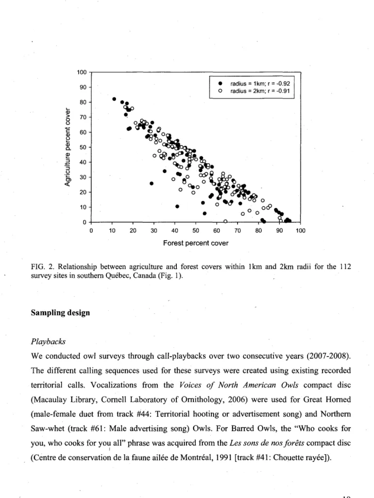
same bird. Stations also needed to keep a minimum 200-m distance from nearby houses to avoid disturbing the owners and reduce interference from dog barking. We selected sites that allowed the coverage of a large agriculture-forest gradient (i.e., 20% to 80% agriculture within a 2-km radius) to compare agriculture versus forest-dominated landscapes (Fig. 2).

s-1

s

p*^ v

. * • • • •>;"':'»*«.

~o?—~jc

FIG. 1. Distribution of the 112 sites surveyed for owls in 2007-2008 in southern Quebec, Canada. Black and white circles indicate site locations. Land cover types include forest (white), disturbed forest (light gray), agriculture (mid-tone gray), urban (dark gray), and water (black). Coordinate units are UTM.

100 90 80 <D > o o c CD o I— Q . (1) 3 3 O 1— TO < 70 60 50 40 30 20 10 0 - ' •

• -v.

Forest percent cover

80 90 100

FIG. 2. Relationship between agriculture and forest covers within 1km and 2km radii for the 112 survey sites in southern Quebec, Canada (Fig. 1).

Sampling design

Playbacks

We conducted owl surveys through call-playbacks over two consecutive years (2007-2008). The different calling sequences used for these surveys were created using existing recorded territorial calls. Vocalizations from the Voices of North American Owls compact disc (Macaulay Library, Cornell Laboratory of Ornithology, 2006) were used for Great Horned (male-female duet from track #44: Territorial hooting or advertisement song) and Northern Saw-whet (track #61: Male advertising song) Owls. For Barred Owls, the "Who cooks for you, who cooks for you all" phrase was acquired from the Les sons de nosforets compact disc (Centre de conservation de la faune ailee de Montreal, 1991 [track #41: Chouette rayee]).

We broadcast the calling sequences using an mp3 player (m230 Sansa, SanDisk) and portable sound system (Pignose Lil'PA). The volume of both devices was adjusted to the maximum possible level without distortion. Field tests (n = 5 per species) revealed that our broadcasts could be heard 1070 to 1470 m away by human ear in open areas (GHOW (mean ± SD): 1110 ±33.9m;BDOW: 1416 ± 11.4 m; NSWO: 1458 ± 17.9 m).

Five calling sequences were used: three single species broadcasts ((1) GHOW only, (2) BDOW only, (3) NSWO only) and two Great Horned Owl-treatment broadcasts ((1) GHOW+BDOW, (2) GHOW+NSWO). The single species broadcasts began with one minute of silence allowing the observer to get used to the listening environment. A soft tonality was then heard to indicate the start of data recording. The next minute was silent in order to listen for spontaneously calling individuals. It was followed by a ca. 20 seconds calling bout during which one vocalization was broadcast at 45, 135, 225 and 315 degrees from the road (in the case of NSWO, the continuous 20-s call was broadcast for 5s in every direction). This was followed by one minute of silence to listen for responding individuals. This calling-listening sequence was repeated six times and ended with a final 2-min silent listening period. The end of data recording was then marked with a loud tonality. For the GHOW-treatment broadcasts we used the same calling sequence, preceded by one minute of silent listening and two minutes of continuous GHOW calls, after which the official data recording period began. The total survey (data recording) duration was 10 min for GHOW, NSWO and GHOW+NSWO broadcasts, and 10.5 min for BDOW and GHOW+BDOW broadcasts.

Owl surveys

We tested each of the 5 calling sequences twice at every site, for a total of 10 visits per site per year. All surveys were conducted from one hour to nine hours after sunset. Survey routes were planed to limit the instances where a site would be visited at the same hour twice. All data were collected under good weather conditions: temperature > -25°C, wind < 15km/h, and with no or very light precipitations (Appendix 1). A minimum 7-day interval separated each visit to the same site so as to avoid owls' habituation to broadcasts. For both years, surveys were performed by two observers working on their own. Each observer visited every site and

broadcast every calling sequence at random dates and hours. Only one observer conducted surveys in both years.

The calling sequences were broadcast according to the owls' calling activity pattern. Great Horned Owls seem to be more vocally active during the month of December through March (Johnsgard 2002), while Barred Owls are mostly heard through the months of February to April, with a peak in late March and April (Mazur and James 2000, Johnsgard 2002). Although Great Horned and Barred Owls may be heard throughout the year, Northern Saw-whet Owls are only vocally active between March and May since they remain mute while wintering and during migration (Johnsgard 2002). Hence, GHOW, BDOW and GHOW+BDOW calling sequences were broadcast randomly between 1 February and 30 May in 2007 and between 14 January and 20 May 2008. NSWO and GHOW+NSWO calling sequences were broadcast randomly after the first Northern Saw-whet Owls were detected in the field: between 23 March and 30 May in 2007 and between 10 March and 20 May 2008.

Data collection

Every time an owl was detected, we recorded the species, the minimum possible number of individuals, and the type of detection (auditory or visual). For each visit, we also recorded the Julian date, hour, temperature, wind speed, and noise level. Temperature (±1°C) and wind speed (±3% of reading) were measured using a Kestrel 2000 Pocket Weather Meter (Nielsen-Kellerman). To estimate noise level, we developed an index that combines two types of -distraction: car disturbance and background noise. First, we counted each car that drove beside

us during the survey and multiplied this number by 4 to get the car disturbance level. Then, each background noise heard during the survey was recorded into a category: background circulation, snowmobiles, wind, running water, dogs, frogs or other. Each noise was further classified into frequency (never: 0, punctual: 1, intermittent: 2, constant: 4) and intensity (silence: 0, soft: 1, moderate: 2, loud: 3) levels. For each noise category, we multiplied the values attributed to frequency and intensity to get the noise level of each category. Noise levels of every category were then added to obtain the total background noise. Finally, the previously estimated car disturbance level was added to the total background noise to get the

survey's total noise level estimation. Although we are aware this noise index is arbitrary, we think it is representative of the noise disturbance experienced during the survey. Since it was demonstrated that background noise decreases detection probability (Pacifici et al. 2008), we thought it was important to consider it in our analysis.

Landscape characterization

Land cover of the study area was obtained through georeferenced, classified Landsat-7 satellite images taken between August 1999 and May 2003 (resolution: 25 m x 25 m; Canadian Wildlife Service 2004). We divided land cover into six categories: (1) forest (deciduous, mixed and coniferous woodlands), (2) disturbed forest (regenerations, burns, cuts), (3) agriculture (croplands, pastures, hayfields, fallows), (4) water (rivers, lakes), (5) wetland (bogs, swamps, marshes), and (6) urban (roads, bare ground, airports, borrow pit, quarry, golf, urban parks, villages, cities) using ArcView GIS Spatial Analyst 2.0 (ESRI 2005). FRAGSTATS 3.3 (McGarigal et al. 2002) was used to calculate the percent cover of every category around each site within a 1-km radius for Great Horned and Northern Saw-whet Owls and a 2-km radius for Barred Owls. We chose the radii based on the owls' home range size. We estimated the average home range radii to be ~0.72km for Great Horned Owls (Houston et al. 1998), ~1.13km for Barred Owls (Mazur and James 2000), and ~0.69km for Northern Saw-whet Owls (Cannings 1993). Since our sites had little chance of being situated at the center of the owl's actual home range, we found it would be suitable to double those radii so as to ensure the analyzed area would encompass as much of the home range as possible. In addition, when choosing a territory, owls may also consider surrounding habitats and the presence of conspecifics (Addicott et al. 1987, Dunning et al. 1992, Andren 1994). Thus, doubling the radii allowed us to include some of the home range's surrounding habitats into the analysis.

Statistical analyses

In addition to our three study species, the presence of one Eastern Screech-Owl {Megascops

asio) individual was recorded on five visits at the same site in 2007 and once at a neighboring

site in 2008. However, only Great Horned, Barred and Northern Saw-whet Owls were considered for data analysis. Furthermore, the number of surveyed owls per visit was low (mostly 1 or 2), preventing us from achieving abundance analysis. Hence the minimum possible number of individuals was converted into simpler presence-absence (0 or 1) data. We estimated the occurrence of owls using PRESENCE 2.2 (Hines 2006) which allows simultaneous estimation of occurrence and detection probability following MacKenzie et al. (2002). A single-species analysis was performed separately for each year and each species. Although multiple-species or multiple-season analyses would have been more appropriate, these model types did not converge. In fact, the method proposed by MacKenzie et al. (2002) to account for imperfect detection uses complex algorithms that are sensitive to colinearity problems. Hence, a very low detection probability or an increase in the number of variables in a model may lead to convergence problems.

Assumptions

Four assumptions had to be followed in single-species analysis (MacKenzie et al. 2006). First, the sites are considered "closed" to changes in occupancy during the entire sampling season (i.e.: no extinctions or colonizations). In this study, the analyses were performed separately for the two years of data collection. Moreover, since our surveys were performed during the breeding season, when owls remain within the same territory and actively defend it from intruding individuals (Johnsgard 2002), we are confident that this first assumption was met. Second, the probability of occupancy is the same for all sites, and third, the probability of detection, given the species is present, is constant across all sites. These two assumptions can be relaxed if differences in occupancy and detection probabilities are modeled as function of covariates (e.g., including a forest cover variable when estimating occupancy and a temperature variable for detection), which is what was done here. Finally, detection histories and detection of species at each site are independent. Given that our sites were spaced so as to

prevent double-sampling and that each visit to the same site was achieved with a minimum 7-day interval, we feel secure that this last assumption was respected.

Models

For each owl species, we built a series of models that shared a fixed set of detection covariates combined with a variety of occurrence covariates (Table 1 and 2). All detection and occurrence covariates were centered on the mean to ease convergence of models. Nevertheless, convergence was not reached for Great Horned Owl 2007 and Northern Saw-whet Owl 2008 possibly due to low detection probability. Thus, only Barred Owl was analyzed in both years. Moreover, one site was removed each from the Barred Owl 2008 and Great Horned Owl 2007 analyses since exceptionally high detection rates occurred at these sites, preventing proper model fitting. For any given model, Pearson product-moment correlations (r) among explanatory variables ranged between -0.53 and 0.41 with the exception of Julian day and temperature which were strongly correlated (0.75 < r < 0.82). However, we decided to keep both variables since they are both believed to influence owl detectability (Takats and Holroyd 1997, Takats et al. 2001) and did not cause colinearity problems when estimating parameters. To be sure, we compared the values of a model including both variables with a model including either Julian day or temperature. When both variables were included in the model, the standard errors were not inflated.

TABL E 1 . Explanator y variable s use d t o asses s th e occurrenc e an d detectio n probabilit y o f Grea t Horne d (GHOW) , Barre d (BDOW ) an d Norther n Saw-whe t (NSWO ) Ow l i n 200 7 an d 200 8 withi n agricultura l landscape s o f souther n Quebec , Canada . Variabl e Abbreviatio n Justification s Specie s Occurrenc e Fores t coye r (%) A Disturbe d fores t cove r (% ) Wetlan d cove r (% ) B ' c Grea t Horne d Ow l occurrenc e Barre d Ow l occurrenc e fo r distur b we t GHOWoc c BDOWoc c Importan t fo r nesting , roosting , an d foragin g (Johnsgar d 2002 ) Shoul d b e avoide d b y BDO W an d NSW O (Canning s 1993 , Mazu r an d Jame s 2000 , Johnsgar d 2002 ) Ofte n associate d wit h BDO W an d NSW O (Canning s 1993 , Mazu r an d Jame s 2000 , Johnsgar d 2002 ) • . BDO W an d NSW O shoul d avoi d habitat s wher e GHO W i s presen t sinc e i t i s thei r predato r an d competito r (Canning s 1993 , Bosakowsk i an d Smit h 1998 , Housto n e t al . 1998 , Mazu r an d Jame s 2000 , Johnsgar d 2002 ) NSW O migh t avoi d habitat s wher e BDO W i s presen t sinc e the y ar e competitor s (Mazu r an d Jame s 2000 , Johnsgar d 2002 ) Al l Al l Al l BDOW , NSW O NSW O Detectio n BDO W broadcast ° NSW O broadcast 0 GHOW+BDO W broadcast 0 GHOW+NSW O broadcast 0 Dat e (Julia n day) A Tim e sinc e sunse t (hour ) Temperatur e (°C ) Nois e leve l E Observe r bBDO W bNSW O bG H BDO W bG H NSW O Julia n postsu n tem p nois e ob s T o compar e efficienc y o f single - an d multiple-specie s broadcast s T o compar e efficienc y o f single - an d multiple-specie s broadcast s T o compar e efficienc y o f single - an d multiple-specie s broadcast s T o compar e efficienc y o f single - an d multiple-specie s broadcast s Callin g activit y o f owl s ma y chang e accordin g t o tim e o f yea r (Takat s e t al . 2001 , MacKenzi e 2005b ) Callin g activit y o f owl s ma y chang e accordin g t o tim e o f da y (Takat s an d Holroy d 1997 ) Callin g activit y o f owl s ma y decreas e i n col d temperature s (Takat s an d Holroy d 1997 ) Detectio n o f owl s decreas e wit h backgroun d nois e (Pacific i e t al . 2008 ) Detectio n o f owl s ma y var y betwee n differen t observer s (Saue r e t al . 1994 ) Al l Al l Al l Al l Al l Al l Al l Al l Al l A Thes e variable s wer e als o square d t o accoun t fo r possibl e quadrati c relations . B Thi s variabl e wa s considere d i n interactio n wit h th e amoun t o f fores t cove r becaus e th e effec t o f fores t cove r ma y b e amplifie d b y additiona l wetlan d cover . c Thi s variabl e represent s bot h th e wate r (rivers , lakes ) riparia n habitat s an d th e wetland s (bogs , swamps , marshes) . I t wa s compute d a s th e su m o f th e wetlan d percen t cove r an d th e wate r tota l edg e percen t cove r (wate r tota l edg e (m ) x 3 0 (m) / are a (m 2 )) . W e use d 3 0 m assumin g edg e effec t ca n b e observe d u p t o 3 0 meter s int o a patc h (Matlac k an d Litvaiti s 1999) . 0 Thes e variable s ar e dumm y variable s fo r th e callin g sequence s used , wit h th e GHO W broadcas t se t a s th e referenc e callin g sequence . E Nois e inde x o n a leve l o f 1 t o 44 , se e th e Method s sectio n fo r furthe r explanations .

TABL E 2 . Mode l selectio n fo r ow l occupanc y i n agricultura l landscape s o f souther n Quebec , Canada , usin g tw o differen t type s o f analyses . Model s accountin g fo r imperfec t detectio n probabilit y (MacKenzi e e t al . 2002 ) share d th e followin g additiona l detectio n covariates : bBDO W + bNSW O + bGH_BDO W + bGH_NSW O + Julia n + Julian 2 + postsu n + tem p + nois e + obs . Se e Tabl e 1 fo r definition s o f variables . Mode l 200 7 MacKenzi e e t al . (2002 ) AAI Q I w , Logisti c regressio n AAIC C I w, 200 8 MacKenzi e e t al . (2002 ) AAIC c 1 w , Logisti c regressio n AAIC c | Wj Grea t Horne d Ow l (1 ) fo r + for " (2 ) fo r + for 2+ distur b (3 ) for + for 2 + we t (4 ) fo r + for 2 + distur b + we t (5 ) fo r + for 2 + we t + fo r x we t (6 ) fo r + for 2 + distur b + we t + fo r x we t (7 ) Detectio n variable s onl y 0.00 0 1.82 9 2.07 1 3.99 8 3.38 2 5.47 9 0.467 2 0.187 3 0.165 9 0.063 3 0.086 1 0.030 2 4.31 8 6.87 8 6.96 8 9.60 5 9.68 5 12.38 9 0.00 0 0.096 5 0.026 8 0.025 6 0.006 9 0.006 6 0.001 7 0.835 9 0.00 0 2.15 0 1.31 6 3.43 6 3.16 0 5.25 2 0.431 6 0.147 3 0.223 5 0.077 4 0.088 9 0.031 2 Barre d Ow l (1 ) fo r + for " (2 ) fo r + for 2 + distur b (3 ) fo r + for 2 + we t (4 ) fo r + for 2 + distur b + we t (5 ) fo r + for 2 + we t + fo r x we t (6 ) fo r + for 2+ distur b + we t + fo r x we t (7 ) fo r + for 2 + GHOWoc c (8 ) fo r + for 2 + distur b + GHOWoc c (9 ) fo r + for 2 + we t + GHOWoc c (10 ) fo r + for 2 + distur b + we t + GHOWoc c (11 ) for + for 2 + we t + fo r x we t + GHOWoc c (12 ) for + for 2 +distur b + we t + fo r x we t + GHOWoc c (13 ) Detectio n variable s onl y 2.46 6 3.57 0 5.21 1 6.28 6 0.00 0 4.04 1 3.54 0 6.07 6 7.87 5 8.85 1 2.32 0 4.92 6 14.88 2 0.123 6 0.071 2 0.031 3 0.018 3 0.424 1 0.056 2 0.072 2 0.020 3 0.008 3 0.005 1 0.133 0 0.036 1 0.000 2 2.62 5 3.76 1 4.77 5 . 5.93 0 0.00 0 2.16 4 4.30 5 5.47 1 6.49 7 7.66 3 1.73 9 3.94 0 0.099 5 0.056 4 0.034 0 0.019 1 0.369 8 0.125 3 0.043 0 0.024 0 0.014 4 0.008 0 0.155 0 0.051 6 0.00 0 2.67 0 2.25 6 3.23 0 4.10 1 5.00 6 2.35 0 5.06 6 5.02 1 5.95 6 6.94 5 7.79 1 11.30 2 0.388 9 0.102 3 0.125 9 0.077 3 0.050 0 0.031 8 0.120 1 0.030 9 0.031 6 0.019 8 0.012 1 0.007 9 0.001 4 0.24 7 1.59 6 1.82 2 3.39 0 0.00 0 2.20 8 2.29 9 3.70 5 3.96 9 5.58 0 2.23 3 4.48 4 0.202 8 0.103 3 0.092 3 0.042 1 0.229 5 0.076 1 0.072 7 0.036 0 0.031 5 0.014 1 0.075 1 0.024 4 Norther n Saw-whe t Ow l (1 ) fo r + for " (2 ) fo r + for 2 + distur b (3 ) fo r + for 2 + we t (4 ) fo r + for 2 + distur b + we t (5 ) fo r + for 2 + we t + fo r x we t (6 ) for + for 2 + distur b + we t + fo r x we t (7 ) fo r + for 2 + GHOWoc c + BDOWoc c (8 ) for + for 2 + distur b + GHOWoc c + BDOWoc c (9 ) fo r + for 2 + we t + GHOWoc c + BDOWoc c (10 ) fo r + for 2 + distur b + we t + GHOWoc c + BDOWoc c (11 ) fo r + for 2 + we t + fo r x we t + GHOWoc c + BDOWoc c (12 ) fo r + for 2 + distur b + we t + fo r x we t + GHOWoc c + BDOWoc c (13 ) Detectio n variable s onl y 7.26 4 7.36 4 0.06 4 0.00 0 2.00 0 2.43 4 9.48 0 10.15 4 3.67 4 4.06 9 5.25 9 6.29 5 6.13 5 0.008 4 0.008 0 0.307 4 0.317 4 0.116 8 0.094 0 0.002 8 0.002 0 0.050 5 0.041 5 0.022 9 0.013 6 0.014 8 2.55 9 3.13 6 0.00 0 1.56 7 1.01 2 2.46 9 6.28 0 6.61 7 3.80 6 5.28 2 5.03 9 6.42 5 0.085 4 0.064 0 0.306 9 0.140 2 0.185 1 0.089 3 0.013 3 0.011 2 0.045 8 0.021 9 0.024 7 0.012 4 2.31 4 0.57 8 2.58 0 1.83 8 0.00 0 0.02 6 4.15 4 2.91 6 4.95 0 4.53 8 3.45 9 3.61 6 0.068 2 0.162 4 0.059 7 0.086 5 0.216 8 0.214 1 0.027 2 0.050 4 0.018 2 0.022 4 0.038 5 0.035 6

Model selection and multi-model inference

We contrasted models based on the Akaike information criterion, corrected for small sample size (AICC) following Burnham and Anderson (2002). Since none of the models were neatly

superior to the others (w; > 0.95), we performed multi-model inference (Burnham and Anderson 2002). We also calculated the unconditional standard errors and 95% confidence intervals associated with each covariate (Burnham and Anderson 2002). Model goodness-of-fit was assessed following MacKenzie and Bailey (2004) using the most complex model of the set.

Logistic regressions

Wishing to compare the results of analyses that account for detection probability and others that do not, we ran a second version of our analyses using logistic regressions in the R statistical environment (version 2.9.0; R Development Core Team 2009). The same models were used and compared through AICC before performing model averaging.

RESULTS

Under average conditions (Appendix 1), detection probability was relatively low for all species when using conspecific calls (range: 0.11-0.32; Table 3). On the other hand, the occurrence probability was fairly high for all species in average landscapes (Appendix 2) without predators or competitors, (range: 0.43-0.94; Table 3). Northern Saw-whet Owl had the highest occurrence probability and Great Horned Owl the lowest. Occurrence probabilities were 0.13 to 0.49 higher than naive occupancy estimates as it was expected since detection probabilities were < 1 for all species (Table 3). Interestingly, for Barred Owl, occupancy was higher in 2008 but if detection probability was ignored, occupancy would mistakenly have been considered higher in 2007.

TABLE 3. Detection and occurrence probabilities of owls in southern Quebec as estimated following MacKenzie et al. (2002). Naive occupancy estimates (i.e., not corrected for imperfect detection) are also presented. These estimates were obtained under average conditions (Appendices 1 and 2) and using conspecific calls in an average landscape without predator or competitor.

Detection probability (p) Naive occupancy estimate Occurrence probability (VJ/)

Great Horned Owl 2007 0.330 2008 0.166 0.304 0.434 Barred Owl 2007 0.317 0.545 0.679 2008 0.112 0.491 0.881

Northern Saw-whet Owl 2007 0.230 0.455 0.942 2008 0.179

TABLE 4. Effects of detection probability covariates obtained following MacKenzie et al. (2002) and subjected to multi-model inference. Regression coefficients (0) are shown with their unconditional standard errors (SE) and 95% confidence intervals. Note that all values are expressed in logit. See Table 1 for definitions of variables and Table 2 for the set of models.

Parameter intercept (p) bBDOW bNSWO bGH BDOW bGH NSWO Julian Julian2 postsun temp noise obs intercept (p) bBDOW bNSWO bGH BDOW bGH NSWO Julian Julian2 postsun temp noise obs Beta (0) SE 95% CI

Great Horned Owl 2008 -1.614 -1.134 -0.517 -0.149 0.613 -0.002 0.000 0.217 0.020 -0.015 -0.096 Barred O1 -1.996 1.229 -0.088 0.436 -0.221 0.031 0.000 0.005 -0.016 -0.055 -0.607 0.420 0.614 0.572 0.472 0.508 0.009 0.000 0.086 0.030 0.029 0.306 wl 2007 0.317 0.362 0.380 0.383 0.384 0.006 0.000 0.060 0.023 0.023 0.217 -2.436 < 0 < -0.791 -2.338 < 9 < 0.070 -1.639 <9<0.604 -1.073 < 6 < 0.776 -0.382<9< 1.608 -0.019 < 0 < 0.015 -0.001<9< 0.000 0.048 < 0 < 0.386 -0.038 < 9 < 0.077 -0.073 < 9 < 0.042 -0.697 < 9 < 0.504 -2.618 < 0 < -1.375 0.519 < 0 < 1.938 -0.833 < 9 < 0.658 -0.316<0< 1.187 -0.973 < 9 < 0.532 0.019 < 9 < 0.043 -0.000 < 9 < 0.000 -0.113 < 9 < 0.123 -0.060 < 0 < 0.029 -o.ioo < e < -o.oio -1.032 < 0 < -0.182 Beta (0) SE • 95% CI

Northern Saw-whet Owl 2007 -2.544 -0.846 1.335 -0.391 1.181 -0.020 0.000 -0.118 0.071 -0.072 0.169 Barred Owl -3.189 1.117 0.513 0.882 0.138 0.024 0.000 0.077 0.002 -0.085 -0.267 0.419 0.627 0.460 0.552 0.467 0.008 0.000 0.074 0.028 0.027 0.261 2008 0.399 0.457 0.458 0.468 0.474 0.006 0.000 0.066 0.025 0.027 0.239 -3.366 < 0 < - l . 7 2 3 -2.075 < 0 < 0.382 0.434 < 0 < 2.236 -1.472 <0<0.690 0.264 < 0 < 2.097 -0.036 < 9 < -0.003 -o.ooi <e<o.ooo -0.263 < 0 < 0.027 0.016 < 0 < 0.126 -0.125 < 0 < -0.018 -0.342 < 0 < 0.680 -3.970 < 0 < -2.407 0.222 < 0 < 2.013 -0.386<0< 1.411 -0.035 < 6 < 1.800 -0.791 < 6 < 1.067 0.012 <0<0.036 0.000 < 0 < 0.001 -0.052 < 0 < 0.206 -0.047 < 0 < 0.051 -0.139 < 0 < -0.031 -0.736 < 9 < 0.202