O
pen
A
rchive
T
OULOUSE
A
rchive
O
uverte (
OATAO
)
OATAO is an open access repository that collects the work of Toulouse researchers and
makes it freely available over the web where possible.
This is an author-deposited version published in :
http://oatao.univ-toulouse.fr/
Eprints ID : 15536
URL :
http://content.iospress.com/articles/informatica/inf23-3-08
To cite this version
: Tchangani, Ayeley and Bouzarour-Amokrane, Yasmina
and Pérès, François Evaluation Model in Decision Analysis: Bipolar
Approach.
(2012) Informatica, vol. 23 (n° 3). pp. 461-485. ISSN 0868-4952
Any correspondence concerning this service should be sent to the repository
administrator:
[email protected]
Evaluation Model in Decision Analysis:
Bipolar Approach
∗
Ayeley P. TCHANGANI
1, Yasmina BOUZAROUR-AMOKRANE
2,
François PÉRÈS
3Université de Toulouse – Laboratoire Génie de Production 47 Avenue d’Azereix, 65016 Tarbes, France
1Université Toulouse III – IUT de Tarbes 1 rue Lautréamont, 65016 Tarbes, France 2Université Toulouse III – Paul Sabatier
118 route de Narbonne, 31062 Toulouse, France 3École Nationale d’Ingénieurs de Tarbes
47 Avenue d’Azereix, 65016 Tarbes, France
e-mail: [email protected], [email protected], [email protected]
Abstract.Three main approaches presently dominate preferences derivation or evaluation process in decision analysis (selecting, ranking or sorting options, alternatives, actions or decisions): value type approach (a value function or an utility measure is derived for each alternative to represent its adequacy with decision goal); outranking methods (a pair comparison of alternatives are car-ried up under each attribute or criteria to derive a pre-order on the alternatives set); and decision rules approach (a set of decision rules are derived by a learning process from a decision table with possible missing data). All these approaches suppose to have a single decision objective to satisfy and all alternatives characterized by a common set of attributes or criteria. In this paper we adopt an approach that highlights bipolar nature of attributes with regards to objectives that we consider to be inherent to any decision analysis problem. We, therefore, introduce supporting and rejecting notions to describ attributes and objectives relationships leading to an evaluation model in terms of two measures or indices (selectability and rejectability) for each alternative in the framework of satisficing game theory. Supporting or rejecting degree of an attribute with regard to an objective is assessed using known techniques such as analytic hierarchy process (AHP). This model allows al-ternatives to be characterized by heteregeneous attributes and incomparability between alal-ternatives in terms of Pareto-equilibria.
Keywords:evaluation model, multi-objectives, multi-attributes, analytic hierarchy process,
satisfic-ing games.
1. Introduction and Statement of the Problem
Decision analysis, that is selecting, ranking, classifying or sorting (clustering) alterna-tives, options, actions or decisions (generically referred to as alternatives in this paper),
is probably the main activity of any human being. Some decisions are routinely and do not need sophisticated algorithms to support decision process whereas other decisions need more or less complex processes to reach a final decision. These complex decisions share some features such as: multiplicity of objectives to satisfy, multiplicity of attributes or cri-teria that characterize alternatives, uncertainty, multiplicity of actors, and so on. For these decision situations there is a need to have a procedure or an evaluation model. Two great paradigms are considered in decision analysis literature: multi-criteria or multi-attributes decision making and multi-objectives decision making, see for instance (Antucheviciene
et al., 2011; Bouyssou et al., 2000; Roy and Bouyssou, 1993; Steuer, 1986; Vincke, 1989; Nemura and Klementavicius, 2008; Turskis and Zavadskas, 2010), with sometime a certain confusion between these paradigms. To clarify the position adopted in this paper, let us consider following definition.
DEFINITION1. An objective in a decision analysis problem is something decision maker(s) care about, want to achieve, want to optimize, want to reach, etc. whereas an attribute or a criteria is a feature of an alternative that is used to evaluate this alternative with regard to pursued objectives.
Given previous definition, it becomes obvious that a decision analysis problem can be both multi-criteria/multi-attributes and multi-objectives and this is assumed in this paper. Decision analysis is, in general, a process with many steps such as formulating decision
goalor objectives, identifying attributes that characterize potential alternatives that can respond to the decision goal and making recommendation regarding these alternatives given the decision goal. The final recommendation step in a decision process can be reduced to three main processes: choosing (this is a relative evaluation that finds a subset, possibly reduced to a singleton, of alternatives that satisfy the decision goal), ranking (relative evaluation that ranks alternatives from the best to the worst with regard to the decision goal) or sorting (an absolute evaluation that sorts alternatives according to a prescribed norm regarding the decision goal). The construction of an evaluation model, often carried by an expert known in the literature as the analyst (Bouyssou et al., 2000) is then an important step in the decision process; this step is the main purpose of this paper. Indeed, we consider that the upstream processes have been considered and we are in possession of the set of alternatives, the consequences tree, attributes measures and our duty is to construct an evaluation model, thus we act as an analyst for the final recommendation. The purpose of this paper is to derive an evaluation model for mainly selecting and/or ranking process in order to achieve multiple objectives; this decision making context is summarized by the following definition.
DEFINITION2. The decision making problem considered here consists in 3-uples
hU, A, Oi where:
• U is a discrete set of n alternatives
• A is a discrete set of m attributes or criteria
A = {a1, a2, . . . , am} ; (2)
• O is a discrete set of k objectives to satisfy that resume the overall decision goal
O = {o1, o2, . . . , ok} . (3)
A decision making problem as defined previously can represent practical situations in many domains such as management, engineering, economics, politics (see for in-stance Geldermann and Rentz (2003) for an application in e-democracy) etc.; inter-ested readers can consults following publications (Antucheviciene et al., 2011; Bouys-sou et al., 2000; Nemura and Klementavicius, 2008; Roy and BouysBouys-sou, 1993; Steuer, 1986; Vincke, 1989; Tchangani, 2009; Turskis and Zavadskas, 2010; Kanapeckiene et al., 2011) and references therein for some real world applications. Applications may also be found in society protection and emergency management such as decision making related to protection against fire (Vaidogas and Sakenaite, 2011) or in human-machine interface design (Kabassi et al., 2005); multicriteria classification problems as decision making problems are encountered in many domains such as finance (Doumpos et al., 2001), among others. The context considered here is different from the case where one want to form a portfolio of alternatives such as in projects management, see for instance Liesio
et al.(2007, 2008), because we do not consider relationships between alternatives. Classically, three main approaches have dominated evaluation process in decision analysis: value type approach (a value function or an utility measure is derived for each alternative to represent its adequacy with decision goal); outranking methods (a pair com-parison of alternatives are carried up under each attribute or criteria to derive a pre-order on the alternatives set); and decision rules approach (a set of decision rules are derived from a decision table with possible missing data). All these approaches suppose to have a single objective to satisfy and a common attributes set for alternatives. These approaches are briefly described below.
• Value type approach: roughly speaking these techniques consider a numerical func-tion π (known as value or utility funcfunc-tion) defined on the alternatives set U such that
π(u) > π(v) ⇔ u% v, u, v∈ U, (4) where “u % v” stands for “u is at least as good, with regard to decision goal, as v” leading to an order on U. The evaluation modeling process then consists in build-ing such a function based on attributes measures and decision makers preference (obtained in general by answering some particular questions of the analyst); there are many techniques employed in the literature for constructing such a function where a number of them suppose a particular form for π such as an expected utility form or an additive value function (interested reader may consult (Bouyssou et al.,
2000; Roy and Bouyssou, 1993; Jacquet and Sisko,1982; Steuer, 1986; Vincke, 1989) and references therein and AHP approach (Saaty, 1980) and its variation to take into account particular relationships between components of decision process (Basak, 2011).
• Outranking methods: a pair comparison of alternatives is carried up under each attribute or criteria to derive a pre-order on the alternatives set U allowing in-comparability and/or intransitivity; methods such as ELECTRE procedures and PROMETHEE techniques (Bouyssou et al., 2000; Roy and Bouyssou, 1993; Vincke, 1989) belong to this category.
• Decision rules approach: a set of decision rules are derived by a learning process from a known decision table with possibly incomplete data (Geco et al., 2001). To take into account some particular aspects of decision making process such as se-quentiality or fuzziness of data, researchers are developing methods to deal with these issues, see for instance Ouerdane et al. (2011) for argumentation approach and Ramik and Perzina (2010) for fuzzy multicriteria decision problems. Some effort is also paid to the estimation of judgements or quantitative and subjective criteria weighting process (Monat, 2009).
In this paper we adopt an approach that highlights the bipolarity of attributes with re-gards to objectives that we consider to be inherent to any decision analysis problem. We are motivated by the fact that cognitive psychologists have observed for long time that hu-man, often, evaluate alternatives by considering separately their positive aspects and their negative aspects; that is on a bipolar basis, see for instance Caciopo and rnston (1994) and Osgood et al. (1957); this view is also common in computer science for informa-tion representainforma-tion (Dubois and Fargier, 2006). To this end, we introduce supporting and
rejectingnotions (Tchangani, 2010) that relate attributes to objectives leading to an eval-uation model in terms of two measures or indices (selectability and rejectability) for each alternative in the framework of satisficing game theory (Stirling, 2003). These notions permit to partition criteria or attributes set into three subsets given an objective: attributes that support this objective, attributes that reject this objective and attributes that are neu-tral with regard to this objective; of course only supporting and rejecting attributes are interesting for evaluation process. Supporting and rejecting degrees of an attribute with regard to an objective are assessed using known techniques such as analytic hierarchy process (AHP). In fact any method, such as performance value analysis (Gurumurthy and Kodali, 2007), that could assign a measure to an attribute with regard to a pair of objective and alternative can be used; here we choose to use AHP approach because of its ability to deal with hierarchy (which permits to decompose attributes from more general statements to more measurable or comparable attributes) and intangible variables. This model allows alternatives to be characterized by heterogeneous attributes and incomparability between alternatives in terms of Pareto-equilibria. Indeed, decision making situations where al-ternatives are characterized by attributes of different nature are pervasive in real world applications. One may think about a government evaluating projects that belong to dif-ferent domains such health, infrastructures, social, economics with the main objective to enhance a country developing process or an enterprise planning to invests in projects
of different nature. In these situations, though attributes characterizing projects may be completely different, the important thing is their adequacy with regards to the pursued objectives, so that the alternative projects can be ultimately compared on the same basis (decision maker desires).
The remainder of this paper is organized as follows: in the Section 2, modelling and assessment of supporting and rejecting relationships between attributes and objectives is considered through analytic hierarchy process (AHP); Section 3 is devoted to evaluation and recommendation procedures using satisficing game; Section 4 considers an illustra-tive application and Section 5 concludes the paper.
2. Modelling and Assessment of Bipolar Relationships
2.1. Modelling
As mentioned in previous section, cognitive psychologists noticed for long time that hu-mans generally evaluate alternatives in decision process by comparing pros and cons of each alternative with regard to decision goal. Building on this observation, we define a supporting/rejecting relationship between attributes and objectives as given by the fol-lowing definition.
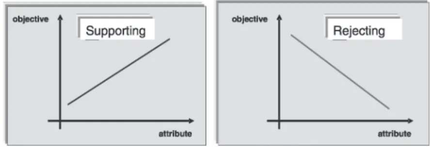
DEFINITION3. An objective ojis said to be supported (respect. rejected) by an attribute
aiif and only if its variation is positively (respect. negatively) correlated with the variation
of that attribute as illustrated by the following Fig. 1. Otherwise this attribute is said to be neutral with regard to that objective.
Fig. 1. Illustration of supporting and rejecting relationships between objectives and attributes.
Given a decision problem as defined in the previous section, for each objective oj,
the set of attributes A1 will be partitioned into A
S(oj), the set of attributes that
sup-port objective oj, AR(oj) the set of attributes that reject oj,and AN(oj) attributes that
1In the case where alternatives are characterized by heteregeneous attributes, this set will depend on alter-native.
are neutral with regards to oj; supporting, rejecting and neutral notions define
equiv-alence relations over the attributes set given an objective. The basis of this approach has been laid in Tchangani (2009) with “positive” and “negative” attributes notions and in Tchangani and Pérès (2010) where authors suggest to elicit and assess attributes in a decision analysis by partitioning them into benefit (B): certain attributes that support decision objective; opportunity (O): uncertain attributes that support decision objective; cost (C): certain attributes that reject decision objective; and risk (R): uncertain attributes that reject decision objective; leading to a framework known as BOCR analysis. The next step towards the establishment of an evaluation model is to assess the strength of each de-fined relationship; this process is carried up in the next subsection using mainly analytic hierarchy process (AHP).
2.2. Bipolar Relationships Strength Assessment Using AHP
The basic AHP (Saaty, 1980), decomposes a decision problem in different elements grouped in clusters that it arranges in a linear hierarchy form where the top element of the hierarchy is the overall goal of the decision problem. The hierarchy goes from the general to more particular until a level of operational criteria against which the decision alternatives can be evaluated is reached. An hierarchy corresponding to our previously defined decision problem may look like that of the following Fig. 2 where ωo is a m
dimension column vector with each entry ωo(o
j) representing the relative importance of
the corresponding objective ojwith regard to the overall decision goal.
The vector ωocan be obtained using the AHP procedure by answering questions of
the form “how important is objective okcompared to the objective olwith regard to the
overall decision goal ?”using the scale given by the weights of Table 1 (Saaty, 1980) to obtain a m × m matrix Ωowhere Ωo(j, l) is the relative importance of objective o
j
com-pared to the objective olwith regard to the overall decision goal. Though, the pair-wise
Table 1
Classical AHP pair-wise comparison weights Verbal scale Numerical values Equally important 1
Moderately more important 3 Strongly more important 5 Very strongly more important 7 Extremely more important 9 Intermediate scales (compromise) 2, 4, 6, 8
comparison matrix Ωocan be constructed arbitrarily and the consistency2 checked later
for possible modifications, there is a straightforward approach that leads to a consistent matrix: one selects a pivot objective opand compare other objectives to this pivot to
ob-tain scores ν(j, p) (from Table 1) for all other objectives j 6= p and then construct the matrix Ωoas shown by equation
Ωo(j, p) = ν(j, p), Ωo(p, j) = 1 ν(j, p), Ωo(j, l) = Ωo(j, p)Ωo(p, l) = ν(j, p)
ν(l, p), (5)
where Ωo(j, l) is the entry of the jth raw and lth column of matrix Ωo; and finally compute
vector ωoas given by (6) ωo(oj) = 1 m m X l=1 µ Ωo(j, l) Pm k=1{Ωo(k, l)} ¶ . (6)
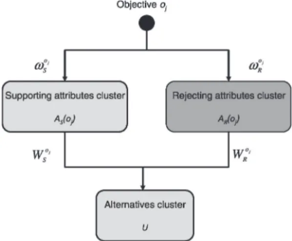
As stated previously, given an objective oj, supporting/rejecting relationships will
partition the set of attributes into AS(oj), the set of attributes that support objective oj
and AR(oj) the set of attributes that reject that objective respectively, so to obtain the
hi-erarchy of Fig. 3. Parameters shown on this Fig. 3 have the following significance: Woj
S
(respectively Woj
R) represents a n×|AS(oj)|3(respectively a n×|AR(oj)|) matrix which
entry Woj
S (ui, ak) for ak ∈ AS(oj) (respectively W oj
R(ui, ak) for ak ∈ AR(oj))
repre-sent the evaluation of alternative uiover the supporting (respectively rejecting) attribute
ak with regard to objective oj; the entries of |AS(oj)| (respectively |AR(oj)|) column
vector ωoj
S (respectively ω oj
R) represent the relative importance of the corresponding
at-tributes with regard to the objective ojin their category.
Weighting vectors ωoj
S and ω oj
R can be determined similar to that of vector ω o by
comparing relative importance of corresponding attributes with regard to the objective oj.
2A pairwise comaprison matrix M is said to be consistent if it verifies M(j, j) = 1, M(j, l) = 1 M(l,j) and M(j, l) = M(j, k)M(k, l).
Fig. 3. Bipolar hierarchy of attributes with regard to objective oj.
For matrices Woj
S and W oj
R there is two possibilities: given an attribute ak,if alternatives
are numerically evaluated over this attribute with ak(ui) the performance of alternative
uiwith regard to akthen the pair-wise comparison matrix Ω oj
× where × stands for S or
Ris obtained by equation Ωak ×(ui, uj) = ak(ui) ak(uj) ; (7)
otherwise this matrix is obtained using a AHP procedure as previously stated by answer-ing a question of the form “how well does perform alternative uicompared to alternative
ujwith regard to attribute ak?”and finally the entry W oj ×(ui, ak) is obtained by equation Woj × (ui, ak) = 1 n X j µ Ωak ×(ui, uj) P kΩ ak ×(uk, uj) ¶ . (8)
A more complete model can be derived by using analytic hierarchy process (ANP) to cope with possible reflexivity relationships that may exist between elements within a same cluster (Saaty, 2005); this approach has been considered in Tchangani (2006) in the framework of satisficing game theory to establish a new multi-attributes decision approach.
In the next section, the final procedure of evaluation and recommendation will be considered.
3. Evaluation and Recommendation Procedures
Bipolar nature of attributes with regard to objectives suggest an evaluation model to-wards two direction: the achievement of objectives and forces competing this achieve-ment. Evaluation process that consists in confronting positive and negative aspects of
alternative is common in human decision making activities in almost all socioeconomic domains; the formalization of such practices is therefore necessary. An interesting frame-work for this formalization is the satisficing game theory; so this section begins by recall-ing basics of this theory that are relevant to the purpose of this paper and then used them to establish the ultimate evaluation and recommendation procedures of the considered decision problem.
3.1. Satisficing Game Theory
The main philosophy of satisficing game theory relies on the fact that, most of the time humans content themselves with alternatives that are just “good enough” because their cognitive capacities are limited and information in their possession is almost always im-perfect; this is the fundamental idea behind the theory of bounded rationality that has its roots in the work by Simon (1997); the concept of being good enough allows a certain flexibility because one can always adjust its aspiration level. This concept is suitable for the approach considered in this paper as being good enough for an alternative can simply signify that the supporting contribution exceeds the rejecting one in some sense. This way of evaluation falls into the framework of praxeology or the study of theory of practical activity (the science of efficient action). For a universe U of alternatives, one will define for each alternative u ∈ U, a selectability function or measure µS(u) and a
rejectabil-ity functionor measure µR(u) to measure the degree to which u works towards success
in achieving the decision maker’s goal and costs associated with this alternative respec-tively. This pair of measures called satisfiability functions are mass functions (they have the mathematical structure of probabilities; Stirling, 2003): they are non negative and sum to one over U. The following definition then gives the set of alternatives arguable to be “good enough” because for these options, the “benefit” expressed by the function µS
exceeds the cost expressed by the function µRwith regard to an index of caution q.
DEFINITION4. The satisficing set Σq ⊆ U is the set of alternatives defined by the
fol-lowing equation
Σq =©u ∈ U: µS(u) > qµR(u)ª. (9)
The caution index q can be used to adjust the aspiration level: increase q if too many alter-natives are declared satisficing or on the contrary decrease q if Σqis empty for instance.
But for a satisficing alternative u there can exist other satisficing alternatives that are better (having more selectability and at most the same rejectability or having less rejectability and at least the same selectability) than u; it is obvious that in this case any rational decision maker will prefer the later alternatives. So the interesting set is that containing satisficing alternatives for which there are no better alternatives: this is the
satisficing equilibriumset ES
q. To define this set, let us define first, for any alternative
equation
D(u) = DS(u) ∪ DR(u), (10)
where DS(u) and DR(u) are defined by equations
DS(u) =©v ∈ U: µR(v) < µR(u)&µS(v) > µS(u)ª, (11)
DR(u) =©v ∈ U: µR(v) 6 µR(u)&µS(v) > µS(u)ª. (12)
The equilibrium set E (alternatives for which there are no strictly better alternatives), which can not be empty by definition, is defined by equation
E =©u ∈ U: D(u) = ∅ª, (13) and the satisficing equilibrium set, ES
q is given by equation
ES
q= E ∩ Σq. (14)
Notice that ES
q constitutes a Pareto-equilibria set so that there is incomparability between
a pair of alternatives in this set, so that a trade-off process is necessary for final choice purpose for instance.
Defining a decision analysis problem as a satisficing game return to finding a way to derive satisfiability measures; the following paragraph presents how to compute these measures for decision problem considered in this paper.
3.2. Satisfiability Functions of the Considered Decision Problem
The stepping stones of a satisficing game are satisfiability measures or functions. Using materials obtained in modelling and assessment section, satisfiability measures can be derived straightforwardly as given by the following definition.
DEFINITION5. The satisfiability functions µSand µRare defined by equations
µS(ui) = X oj∈O ½ ωo(oj) ½ X ak∈AS(oj) ©ωoj S(ak)W oj S (ui, ak) ª ¾¾ , (15) µR(ui) = X oj∈O ½ ωo(oj) ½ X ak∈AR(oj) ©ωoj R(ak)W oj R (ui, ak) ª ¾¾ . (16)
It is obvious that µS and µRfulfill the requirements of satisfiability measures. Based
on these measures, one will obtain the satisficing equilibria set ES
q from which a final
alternative can be selected in the case of choosing process; the following paragraph con-siders some possible recommendation procedures. Of course, one can imagine other pos-sibilities.
3.3. Recommendation Procedures
Choosing and ranking are relative evaluation operations (Bouyssou et al., 2000) over the alternatives set U; based on the previously derived materials, an obvious value function π(u), ∀ u ∈ U can be defined as a function of the satisfiability measures µS(u) and
µR(u), that is
π(u) = π¡µS(u), µR(u)¢, (17)
which can take particular form depending on the decision goal. Here is some of these possible forms
π(u) = µS(u) − qµR(u), (18)
that gives the priority to alternatives with large difference between the selectability mea-sure and the rejectability meamea-sure given the index of caution q, or
π(u) = µS(u) µR(u)
, (19)
that considers alternatives with the largest index of caution, or
π(u) = µS(u) µ respect.π(u) = 1 µR(u) ¶ , (20)
that gives priority to alternatives with the largest selectability (respect. lowest rejectabil-ity); this later case is suitable when one of the measure is uniformly distributed over alternatives. This value function can then be used to select the ultimate alternative u∗as
shown by equation
u∗= arg max
v∈ES q
π(v), (21)
or to rank alternatives using the relation given by equation
uº v ⇐⇒ π(u) > π(v). (22) Sorting is an absolute operation (Bouyssou et al., 2000) that requires defining norms and categories; different norms can be derived by using the value function π(u). For instance, in the case π(u) = µS(u) − qµR(u), two natural partitions of U are given by
equation
C1= Σq=©u ∈ U: π(u) > 0ª and C2= U − C1. (23)
Besides this possibility of sorting, the satisficing game approach leads to a natural cate-gorization of the alternatives set U into four subsets, namely ES
U − Σq ∪ E. In terms of preference the subset EqS is obviously preferred to the rest: it
contains alternatives arguable to be “best good enough” (their selectability exceeds their rejectability and there are no alternatives that are better than them) and the set U − Σq∪ E
contains completely inefficient alternatives (they are not satisficing alternatives nor equi-librium); there is no obvious conclusion for the subsets E − ES
q and Σq − EqS and a
sensitivity analysis can be done for these alternatives, see for instance Tchangani (2009). To show the applicability of the approach established so fare step by step, we consider a decision problem in manufacturing domain; the purpose here is to choose or justify the best practice in terms of manufacturing management model (technology oriented model, management oriented model or traditional model).
4. Example of Application
4.1. Description
The materials of this application are extracted from Gurumurthy and Kodali (2007) and Gurumurthy and Kodali (2008) and adapted to the approach established in this paper. In Gurumurthy and Kodali (2007) and Gurumurthy and Kodali (2008), a performance value analysis approach is used to justify the adoption of a management oriented man-ufacturing approach in terms of lean manman-ufacturing system (LMS) in comparison to a technology oriented manufacturing approach such as computer integrated manufacturing system (CIMS) and a traditional manufacturing system (TMS) using some indicators such as productivity, competitiveness, flexibility, innovation, etc. which are evaluated through a certain number of attributes obtained through interviews of managers. The result was that using these indicators and performances of attributes for each of these three manu-facturing systems, LMS outranks CIMS that in return outranks TMS. To conform to the framework established in this paper we re-organize the materials from Gurumurthy and Kodali (2007) and Gurumurthy and Kodali (2008) as given in the following paragraphs. 4.1.1. Objectives
We have identified five objectives that correspond to main indicators considered in Guru-murthy and Kodali (2007) and GuruGuru-murthy and Kodali (2008); they are:
• o1– productivity objective, • o2– social objective, • o3– competitiveness objective, • o4– flexibility objective, • o5– innovation objective. 4.1.2. Alternatives
There are obviously 3 alternatives as stated previously defined as: • u1– traditional manufacturing system (TMS);
• u2– technology oriented system in terms of computers integrated manufacturing
system (CIMS);
4.1.3. Attributes
Different attributes used in Gurumurthy and Kodali (2007) and Gurumurthy and Kodali (2008) for each objective are reorganized in terms of supporting and rejecting and their performance matrices as well as normalized matrices Woj
× and weights ω oj
× given below.
4.1.3.1. Attributes to evaluate productivity objective
Supporting attributes of productivity objective
• Labour productivity (LAP, in %).
• Number of inventory or stock rotations (SRO, in Nos.). • Production capacity (PRC, in number of units per year). • Overall Equipment Efficiency (OEE, in %)).
• Equipment utilization (EQU, in %). • Overall productivity (OPR). • Labour utilization (LAU, in %). • Utilization of capacity (UTC, in %). • Production rate (PRR).
• Production volume (PRV).
• Material productivity (MAP, in %). • Machine productivity (MCP, in %). • Value added time (VAT, in hours).
• Average operation time per week (AVT, in days). • Reliability of machines (REL, in %).
Performance matrix for supporting attributes of productivity objective (Table 2) Rejecting attributes of productivity objective
• Manufacturing cycle time (MCT, in hours). • Total floor space (TFS, in m2).
• Number of stages in the overall material flow (RNS, in Nos.). • Number of bottleneck stages (NOB, in Nos.).
• Maintenance time (RMT, in hours per week). • Non value added time (NVA, in days).
• Percentage of unscheduled downtime or equipment breakdown time (USD, in %). • Takt time (TAK, in hours).
Performance matrix for rejecting attributes of productivity objective (Table 3)
4.1.3.2. Attributes to evaluate social objective
Supporting attributes of social objective
• Number of awards and rewards provided for workers (REC, in Nos.).
• Percentage of inspection carried out by autonomous defect control (ICA, in %). • Number of teams (TEA, in Nos.).
• Percentage of employees working in team (EWT, in %). • Reduction in number of workers (RNW).
Table 2
Supporting attributes of productivity objective Attributes TMS CIMS LMS Attributes
weights LAP 78 90 85 1 SRO 6 10 12 1 PRC 10, 000 14, 000 11, 000 1 OEE 42 65 75 1 EQU 73 80 85 1
OPR Low Medium High 1
LAU 86 80 90 1
UTC 83 85 80 1
PRR Low High Medium 1 PRV Low High Medium 1
MAP 82 85 90 1 MCP 78 85 90 1 VAT 4.5 6 6.5 1 AVT 4.1 5 5.51 1 REL 74 85 80 1 Wo1 S ω o1 S LAP 0.3083 0.3557 0.3360 0.0667 SRO 0.2143 0.3571 0.4286 0.0667 PRC 0.2857 0.4000 0.3143 0.0667 OEE 0.2308 0.3571 0.4121 0.0667 EQU 0.3067 0.3361 0.3571 0.0667 OPR 0.0667 0.3333 0.6000 0.0667 LAU 0.3359 0.3125 0.3516 0.0667 UTC 0.3347 0.3427 0.3226 0.0667 PRR 0.0667 0.6000 0.3333 0.0667 PRV 0.0667 0.6000 0.3333 0.0667 MAP 0.3191 0.3307 0.3502 0.0667 MCP 0.3083 0.3360 0.3557 0.0667 VAT 0.2647 0.3529 0.3824 0.0667 AVT 0.2808 0.3425 0.3767 0.0667 REL 0.3096 0.3556 0.3347 0.0667
• Amount of training (TRH, in number of days/year). • Use of visual management or aids (VMA).
• Level of housekeeping (HOK).
• Condition of work environment (WOE). • Worker morale and satisfaction (WMS).
• Communication between employees and management (COM).
Table 3
Rejecting attributes of productivity objective Attributes TMS CIMS LMS Attributes
weights MCT 0.6 0.35 0.4 1 TFS 1200 1000 950 1 RNS 14 12 11 1 NOB 4 2 2 1 RMT 26 28 20 1 NVA 3 2 1 1 USD 33 25 20 1 TAK 0.5 0.35 0.3 1 NVA 3 2 1 1 USD 33 25 20 1 TAK 0.5 0.35 0.3 1 Wo1 R ω o1 R MCT 0.4444 0.2593 0.2963 0.1250 TFS 0.3810 0.3175 0.3016 0.1250 RNS 0.3784 0.3243 0.2973 0.1250 NOB 0.5000 0.2500 0.2500 0.1250 RMT 0.3514 0.3784 0.2703 0.1250 NVA 0.5000 0.3333 0.1667 0.1250 USD 0.4231 0.3205 0.2564 0.1250 TAK 0.4348 0.3043 0.2609 0.1250
Performance matrix for supporting attributes of social objective (Table 4) Rejecting attributes of social objective
• Direct labour (DIL, in Nos.). • Indirect labour (IDL, in Nos.).
• Number of workers/employees (NOW, in Nos.). • Employee turnover rate (ETR).
• Number of shifts or working hours (RWH, in Nos.). • Hierarchy in the organization structure (HIE, in Nos.). • Absenteeism rate (ABM).
• Number of accidents (NOA, in Nos.). • Overtime per week (OVE, in days).
Performance matrix for rejecting attributes of social objective (Table 5)
4.1.3.3. Attributes to evaluate competitiveness objective
Supporting attributes of competitiveness objective
• Gross annual profit (GRP, in lakhs of Rs.). • Total sales (TOS, in lakhs of Rs.).
Table 4
Supporting attributes of social objective Attributes TMS CIMS LMS Attributes
weights
REC 6 8 12 7
ICA 24 90 95 7
TEA 4 6 9 7
EWT 20 50 70 6
RNW Low High Medium 7
TRH 14 24 30 7
VMA Low Medium High 7 HOK Low Medium High 7
WOE P oor F air Good 6
WMS Low Medium High 7 COM Low Medium High 7
PSL 12 15 25 7 Wo2 S ω o2 S REC 0.2308 0.3077 0.4615 0.0854 ICA 0.1148 0.4306 0.4545 0.0854 TEA 0.2105 0.3158 0.4737 0.0854 EWT 0.1429 0.3571 0.5000 0.0732 RNW 0.0667 0.6000 0.3333 0.0854 TRH 0.2059 0.3529 0.4412 0.0854 VMA 0.0667 0.3333 0.6000 0.0854 HOK 0.0667 0.3333 0.6000 0.0854 WOE 0.0667 0.3333 0.6000 0.0732 WMS 0.0667 0.3333 0.6000 0.0854 COM 0.0667 0.3333 0.6000 0.0854 PSL 0.2308 0.2885 0.4808 0.0854
• Revenue (REV, in lakhs of Rs.). • Customer good will (CGW). • Market share (MAS, in %). • Brand image (BRI).
• Dividends paid to shareholders (DTS, in %). • Return on assets (ROA).
• Customer satisfaction (CUS). • Time-based competitiveness (TBC).
Performance matrix for supporting attributes of competitiveness objective (Table 6) Rejecting attributes of competitiveness objective
• Loss of customers (LOC).
• Price of the product (PRI, in lakhs of Rs.). • Lost sales (LOS).
Table 5
Rejecting attributes of social objective Attributes TMS CIMS LMS Attributes
weights
DIL 42 35 35 8
IDL 38 30 35 8
NOW 80 75 70 8
ETR High Medium Low 6
RWH 3 2 2 6
HIE 6 5 4 5
ABM High Medium Low 6
NOA High Low Low 6
OVE 2 1 0.5 7 Wo2 R ω o2 R DIL 0.3750 0.3125 0.3125 0.1333 IDL 0.3689 0.2913 0.3398 0.1333 NOW 0.3556 0.3333 0.3111 0.1333 ETR 0.6000 0.3333 0.0667 0.1000 RWH 0.4286 0.2857 0.2857 0.1000 HIE 0.4000 0.3333 0.2667 0.0833 ABM 0.6000 0.3333 0.0667 0.1000 NOA 0.8182 0.0909 0.0909 0.1000 OVE 0.5714 0.2857 0.1429 0.1167
Performance matrix for rejecting attributes of competitiveness objective (Table 7)
4.1.3.4. Attributes to evaluate flexibility objective
Supporting attributes of flexibility objective
• Availability of reserve capacity (ARC).
• Percentage of flexible employees cross trained to perform three or more jobs (FEM, in %).
• Percentage of production equipment that is computer integrated or automated (AUT, in %).
• Overall flexibility (OFX).
• Number of mixed models in a line (NMM, in Nos.). • Frequency of die changes (FDC).
Performance matrix for supporting attributes of flexibility objective (Table 8) Rejecting attributes of flexibility objective
• Work in process inventory (WIP, in days). • Setup time (SET, in hours).
Table 6
Supporting attributes of competitiveness objective Attributes TMS CIMS LMS Attributes
weights
GRP 240 300 305 10
TOS 550 650 675 9
REV 600 675 700 9
CGW Low Medium High 7
MAS 22 25 28 8
BRI Medium High High 8
DTS 8 10 11 7
ROA Low Medium High 6 CUS Low Medium High 8
TBC Low High High 7
Wo3 S ω o3 S GRP 0.2840 0.3550 0.3609 0.1266 TOS 0.2933 0.3467 0.3600 0.1139 REV 0.3038 0.3418 0.3544 0.1139 CGW 0.0667 0.3333 0.6000 0.0886 MAS 0.2933 0.3333 0.3733 0.1013 BRI 0.2174 0.3913 0.3913 0.1013 DTS 0.2759 0.3448 0.3793 0.0886 ROA 0.0667 0.3333 0.6000 0.0759 CUS 0.0667 0.3333 0.6000 0.1013 TBC 0.0526 0.4737 0.4737 0.0886 Table 7
Rejecting attributes of competitiveness objective Attributes TMS CIMS LMS Attributes
weights LOC Low Medium High 6
PRI 0.6 0.35 0.3 8
LOS High Medium Low 7 Wo3 R ω o3 R LOC 0.0667 0.3333 0.6000 0.2857 PRI 0.4800 0.2800 0.2400 0.3810 LOS 0.0667 0.3333 0.6000 0.3333
Table 8
Supporting attributes of flexibility objective Attributes TMS CIMS LMS Attributes
weights ARC Low Medium High 7
FEM 18 25 30 8
AUT 10 60 20 8
OFX Low Medium High 6
NMM 1 5 5 7
FDC Low Medium High 7 Wo4 S ω o4 S ARC 0.0667 0.3333 0.6000 0.1628 FEM 0.2466 0.3425 0.4110 0.1860 AUT 0.1111 0.6667 0.2222 0.1860 OFX 0.0667 0.3333 0.6000 0.1395 NMM 0.0909 0.4545 0.4545 0.1628 FDC 0.0667 0.3333 0.6000 0.1628
• Finished goods inventory (FGI, in days). • Batch size (BAS).
• Length of product runs (LPR).
• Raw material inventory (RMI, in days).
Performance matrix for rejecting attributes of flexibility objective (Table 9)
4.1.3.5. Attributes to evaluate innovation objective
Supporting attributes of innovation objective
• Number of suggestions per employee per year (SUG, in Nos.). • Percentage of parts co-designed with suppliers (PCS, in %). • Number of new products introduced (NNP, in Nos.). • R&D Expenditure as a percentage of turnover (RDE, in %). • Percentage of common or standardized parts (COP, in %).
Performance matrix for supporting attributes of innovation objective (Table 10) Rejecting attributes of innovation objective
• Time to market for new products (TTM, in years). • Time spent on engineering changes (TEC, in days). • Total parts in Bill of Materials (NOP).
Table 9
Rejecting attributes of flexibility objective Attributes TMS CIMS LMS Attributes
weights
WIP 20 14 10 9
SET 8 6.5 5 10
FGI 12 9 7 9
BAS High Medium Low 8 LPR High Medium Low 7
RMI 15 8 6 9 Wo4 R ω o4 R WIP 0.4545 0.3182 0.2273 0.1731 SET 0.4103 0.3333 0.2564 0.1923 FGI 0.4286 0.3214 0.2500 0.1731 BAS 0.6000 0.3333 0.0667 0.1538 LPR 0.6000 0.3333 0.0667 0.1346 RMI 0.5172 0.2759 0.2069 0.1731 Table 10
Supporting attributes of innovation objective Attributes TMS CIMS LMS Attributes
weights SUG 20 35 55 8 PCS 7 14 20 7 NNP 3 4 5 8 RDE 13 20 22 8 COP 8 14 16 7 Wo5 S ω o5 S SUG 0.1818 0.3182 0.5000 0.2105 PCS 0.1707 0.3415 0.4878 0.1842 NNP 0.2500 0.3333 0.4167 0.2105 RDE 0.2364 0.3636 0.4000 0.2105 COP 0.2105 0.3684 0.4211 0.1842 4.2. Results
From different performance and weights matrices, a AHP analysis through (7) and (8) for each category has been done to obtain the evaluation of each alternative with regard to attributes in terms of matrices Woj
×(ui, ak) and ω oj
Table 11
Rejecting attributes of innovation objective Attributes TMS CIMS LMS Attributes
weights
TTM 4 3.5 3 7
TEC 3 2 1 5
NOP High Medium Low 6 ||cWo5 R ω o5 R TTM 0.3810 0.3333 0.2857 0.3889 TEC 0.5000 0.3333 0.1667 0.2778 NOP 0.6000 0.3333 0.0667 0.3333 Table 12
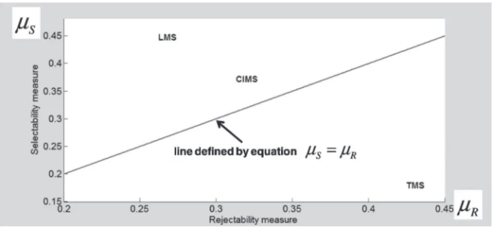
Selectability and rejectability measures for the considered application Satisfiability TMS CIMS LMS
measures
µS 0.1802 0.3721 0.4478 µR 0.4247 0.3133 0.2620
are converted to numerical evaluation using the conversion rules considered in Guru-murthy and Kodali (2007) and GuruGuru-murthy and Kodali (2008), that is Low/Poor = 1;
Medium/Fair = 5; High/Good = 9; finally, considering all objectives to have the same
importance, that is the vector ωois given by equation
ωo=£ 0.2 0.2 0.2 0.2 0.2¤T
; (24)
selectability measure µSand rejectability measure µRare computed by (15)–(16) and the
results are given in the following Table 12 and also depicted on Fig. 4.
Showing alternatives positions in the plane (µR, µS) as Fig. 4, may be of a great
aid for analysis (mainly when there are a great number of alternatives) as this allows to visualize equilibria, satisficing, not satisficing alternatives, and for a particular alternative one can determine alternatives that may dominate it; this information can be used to guide a sensitivity analysis process for trade-off seeking for instance. One can see from Fig. 4 that alternative LMS is the unique satisficing equilibrium at the caution index q = 1 because it dominates the two other alternatives CIMS and TMS; furthermore CIMS dominates TMS so that the ultimate dominance structure is given by equation
Fig. 4. Positions of alternatives in (rejectability, selectability) plane.
where “≻” stands for “is better than”. Given this dominance structure there is no need to use complex recommendation procedures as that developed at Section 3.3 for final decision making.
5. Generalizing Conclusion
The problem of constructing an evaluation model for decision analysis where a certain number of objectives must be satisfied and where alternatives are characterized by multi-ple attributes or criteria is considered in this paper. The philosophy behind the established model highlights bipolarity that characterize relationships between attributes or criteria and objectives in a decision analysis problem. Indeed, given an objective, there will be attributes that work towards the achievement of this objective (referred to as supporting attributes) and attributes that work in the opposite sense (known as rejecting attributes). Given this distinction, an appropriate framework identified in the literature to formulate the evaluation model is that of satisficing game. So the established evaluation model con-sist in separating and aggregating separately, given an alternative, the supporting strength and the rejecting one. Supporting and rejecting relationships degrees are assessed using the well known analytic hierarchy process (AHP). By so doing, though it has not been explicitly considered in this paper, alternatives can be characterized by heterogeneous attributes making it suitable for use in many socioeconomic decision making contexts. Application of the established approach to a real world problem has shown its effective-ness.
References
Antucheviciene, J., Zakarevicius, A., Zavadskas, E.K. (2011). Measuring congruence of ranking results apply-ing particular MCDM methods. Informatica, 22(3), 319–338.
Basak, I.(2011). An alternate method of deriving priorities and related inferences for group decision making in analytic hierarchy process. Journal of Multi-Criteria Decision Analysis, 18(5–6), 279–287.
Bouyssou, D., Marchant, T., Perny, P.,Pirlot, M. , Tsoukiàs, A., Vincke, P. (2000). Evaluation and Decision Models: A critical Perspective, Kluwer Academic, Dordrecht.
Caciopo, J.T., Berntson, G.G. (1994). Relationship between attitudes and evaluative space: a critical review, with emphasis on the separability of positive and negative substrates. Psychological Bulletin, 115, 401–423. Doumpos, M., Zanakis, S.H., Zopounidis, C. (2001). Multicriteria preference disaggregation for classification
problems with an application to global investing risk. Decision Sciences, 32(2), 333–386.
Dubois, D., Fargier, H. (2006). Qualitative decision making with bipolar information. American Association for Artificial Intelligence(www.aaai.org).
Greco, S., Matarazzo, B., Slowinski, R. (2001). Rough sets theory for multicriteria decision analysis. European Journal of Operational Research, 129(1), 1–47.
Geldermann, J., Rentz , O. (2003). Environmental decisions and electronic democracy. Journal of Multi-Criteria Decision Analysis, 12(2–3), 77–92.
Gurumurthy, A., Kodali, R. (2007). Performance value analysis for the justification of lean manufacturing sys-tems. In: Proceedings of the 2007 IEEE IEEM, pp. 377–381.
Gurumurthy, A., Kodali, R. (2008). A multi-criteria decision-making model for the justification of lean manu-facturing systems. International Journal of Management Science and Engineering Management, 3(2), 100– 118.
Jacquet-Lagrèze, E., Sisko, J. (1982). Assessing a set of additive utility functions for multicriteria decision making: the UTA method. European Journal of Operational Research, 10(2), 151–164.
Kabassi, K., Despotis, D.K., Virvou, M. (2005). A multicriteria approach to dynamic reasoning in an intelligent user interface. International Journal of Information Technology & Decision Making, 4(1), 21–34. Kanapeckiene, L., Kaklauskas, A. , Zavadskas, E.K., Raslanas, S. (2011). Method and system for multi-attribute
market value assessment in analysis of construction and retrofit projects. Expert Systems with Applications, 38(11), 14196–14207.
Liesio, J. , Mild, P., Salo, A. (2007). Preference programming for robust portfolio modeling and project selec-tion. European Journal of Operational Research, 181, 1488–1505.
Liesio, J. , Mild, P., Salo, A. (2008). Robust portfolio modeling with incomplete cost information and project interdependencies. European Journal of Operational Research, 190, 679–695.
Monat, J.P. (2009). The benefits of global scaling in multi-criteria decision analysis Judgment and Decision Making, 4(6) 492–508.
Nemura, A., Klementavicius, A. (2008). Multi-criterion assessment of preferences for communication alterna-tives of wind power park information system. Informatica, 19(1), 63–80.
Osgood, C.E., Suci, G., Tannenbaum, P.H. (1957). The Measurement of Meaning. Univ. of Ilinois Press, Chicago.
Ouerdane, W., Dimopoulos, Y., Liapis, K., Moraitis, P. (2011). Towards automating decision aiding through argumentation. Journal of Multi-Criteria Decision Analysis, 18(5–6), 289–309.
Ramík, J., Perzina, R. (2010). A method for solving fuzzy multicriteria decision problems with dependent criteria. Fuzzy Optimization and Decision Making, 9(2), 123–141.
Roy, B., Bouyssou, D. (1993). Aide Multicritère a la Decision: Méthodes et Cas, Edition Economica, Paris (in French).
Saaty, T. (1980). The Analytic Hierarchical Process: Planning, Priority, Resource Allocation. McGraw-Hill, New York.
Saaty, T. (2005). Theory and Applications of the Analytic Network Process: Decision Making with Benefits, Opportunities, Costs, and Risks, RWS Publications.
Simon, H.A. (1997). Administrative Behavior: a study of decision-making processes in administrative organi-zations, 4th edn. The Free Press.
Steuer, R.E. (1986). Muticriteria Optimization: Theory, Computation, and Application. Wiley, New York. Stirling, W.C. (2003). Satisficing Games and Decision Making: With Applications to Engineering and Computer
Science. Cambridge University Press, Cambridge.
Tchangani, A.P. (2006). SANPEV: a satisficing analytic network process framework for efficiency evaluation of alternatives. Foundations of Computing and Decision Sciences Journal, 31(3–4), 291–319.
Tchangani, A.P. (2009). Evaluation model for multi attributes – multi agents decision making: satisficing game approach. International Journal of Information Technology and Decision Making, 8(1), 73–91.
Tchangani, A.P. (2010). Considering bipolarity of attributes with regards to objectives in decisions evaluation. Inzinerine Ekonomika – Engineering Economics, 21(5), 475–484.
Tchangani, A.P., Pérès, F. (2010). BOCR framework for decision analysis. In: Pierre, B. and Gheorghe, F.F. (Eds.) Proceedings of 12th IFAC Symposium on Large Scale Complex Systems Theory and Applications, Vol. 9, Part 1. http://www.ifac-papersonline.net/.
Turskis, Z., Zavadskas, E.K. (2010). A novel method for multiple criteria analysis: grey additive ratio assess-ment (ARAS-G) method. Informatica, 21(4), 597–610.
Vaidogas, E.R., Sakenaite, J. (2011). Multi-attribute decision-making in economics of fire protection. Inzinerine Ekonomika-Engineering Economics, 22(3), 262–270.