Any correspondence concerning this service should be sent to the repository
Administrator :
archiveouverte@ensam.eu
Science Arts & Métiers (SAM)
is an open access repository that collects the work of Arts et Métiers ParisTech
researchers and makes it freely available over the web where possible.
This is an author-deposited version published in:
https://sam.ensam.eu
Handle ID: .
http://hdl.handle.net/null
To cite this version :
Bastien VAYSSETTE, Nicolas SAINTIER, Charles BRUGGER, Mohamed EL MAY, Etienne
PESSARD - Numerical modelling of surface roughness effect on the fatigue behavior of Ti-6Al-4V
obtained by additive manufacturing - International Journal of Fatigue n°123, p.180-195 - 2019
Any correspondence concerning this service should be sent to the repository
Administrator :
archiveouverte@ensam.eu
Keywords: Roughness Surface modelling Additive manufacturing Titanium alloys Fatigue criteria
Selective Laser Melting (SLM) is a powder bed fusion process which allows to build-up parts by successive addition of layers using 3D-CAD models. Among the advantages, the high degree of freedom for part design and the small loss of material explain the increasing number of Ti-6Al-4V parts obtained by this process. However, right after additive manufacturing, these parts contain defects (surface roughness, porosity, residual stresses) which significantly decrease the High Cycle Fatigue (HCF) life. In order to minimize the porosity and residual stresses, post-processing treatments like Hot Isostatic Pressing (HIP) and Stress Relieving (SR) are often con-ducted. But the reduction of the surface roughness by machining is very costly and not always possible, espe-cially for parts with complex geometry. The aim of this work is to evaluate the effect of the surface roughness of Ti-6Al-4V parts produced by SLM on the HCF behavior and to propose a methodology to estimate this effect. Three sets of specimens were tested in tension-compression: Hot-Rolled (reference); SLM HIP machined; SLM HIP as-built. For each condition, microstructure characterization, observation of the fracture surface of broken specimens, surface analysis and volume analysis were carried out respectively by Optical Microscope (OM), Scanning Electron Microscope (SEM), 3D optical profilometer and 3D X-ray tomograph. Results of fatigue testing show a significant decrease of the HCF life mainly due to the surface roughness. Along with experimental testing, numerical simulations using FEM were conducted using the surface scans obtained by profilometry and tomo-graphy. Based on extreme values statistics of a non-local fatigue indicator parameter (FIP), a methodology is proposed to take into account the effect of the surface roughness on the HCF life.
1. Introduction
In order to make the most of the additive manufacturing technolo-gies, the fatigue behavior of additively manufactured materials has to be understood. Due to the quick development of this technology, a limited, yet fast evolving literature exists on this topic. Specimens ob-tained by SLM contain many defects that are inherent to the process and impossible to eliminate even with the best process parameters mon-itoring[1–3]. Among these defects, porosity, surface roughness[4–6]
and residual stresses [7,8] are critical factors regarding the HCF strength.
Depending on their size and morphology, defects may lead to an early fatigue crack initiation. In the case of additive manufacturing it is well known that, before any post-treatment, the HCF strength of as-built specimens is not suitable for aircraft applications[9]. It is usually dif-ficult to quantify and understand the respective influence of these de-fects since in many studies, the early crack initiation is due to a
combination of parameters including porosity, surface roughness, re-sidual stresses and specific microstructures[9–11]. Additively manu-factured parts used for aircraft applications are almost systematically stress-relieved and post processed by HIP which reduces the effect of internal defects on the HCF behavior, but since the pressurizing medium impinges on the surface-connected porosity as though it was an extension of the surface, it does not change the possible impact on surface-connected defects[12]. On the other hand, surface roughness cannot always be removed since the parts may have complex shapes. It is then very important to understand its effect on the HCF strength, and to propose a methodology for fatigue life prediction of rough surface effects under multiaxial loading.
Most of existing models[13–15] accounting for the effect of the surface roughness on the HCF strength consider the surface as a series of micronotches. The theoretical stress concentration factor induced by the notchKt=|σσloc|
nom is introduced, where σlocis the stress at the notch
tip and σnom is the nominal stress. Kt can then be calculated using
https://doi.org/10.1016/j.ijfatigue.2019.02.014
Received 26 October 2018; Received in revised form 21 January 2019; Accepted 11 February 2019 ⁎Corresponding author.
analytical formulations[16]or FEM. Since it is very difficult to measure
the geometrical parameters needed to calculate the stress concentration factor for all the notches, Neuber et al.[13]followed by Arola et al.
[14,15] suggested analytical formulations to obtain the stress con-centration factor based on surface roughness parameters. Theses models have proven efficient in predicting HCF strength. However, they require a periodic and homogeneous surface as obtained by machining and are therefore not applicable to additively manufactured surfaces. More re-cently, As et al. [17] proposed a promising model where the HCF strength is predicted from 2D FEM using 3D topography measurements, the later methodology being applicable even to complex surface morphologies.
After stress relieving and HIP, the HCF behavior of as-built (i.e. rough) parts is governed by different competing factors. First, the sur-face roughness induces local geometrical discontinuities which act as stress concentrators. Secondly, high stress gradients occur resulting in a well known supporting effect regarding the HCF behavior[18,19]. In the case of fatigue prediction of notched structures it is usually con-sidered that the local stress at the notch tip is not suitable for fatigue life evaluation. In the general case, the effect of stress gradient at the notch tip can have several physical consequences, either on the local stress state (the presence of strong gradients modifies the development of local microplasticity as compared to smooth specimens), and, under certain conditions, on the development of non- propagating cracks. In both cases, in order to have cracks to initiate and overcome micro-structural barriers, the stress state has to be sufficiently high over a certain distance (or volume) from the highest loaded point. If not, cracks may initiate without propagating to a critical size from a struc-tural point of view. Such observations were made by Frost et al.[18]
and Smith and Miller [19], who observed non-propagating cracks, measuring one to few grains at sharp notches, for an imposed stress lower than the endurance limit in the case of mild steel. Similar ob-servations were made by Palin-luc et al.[20]in the case of spheroidal graphite cast iron. Different methods can address this issue. Smith and Miller [19], El Haddad [21] and later Murakami [22–24] propose methods based on the Linear Elastic Fracture Mechanics framework. But these methods have shown mostly conservative results for uniaxial tension loading, require costly determination of ΔKth, use the Linear
Elastic Fracture Mechanics although it is a“short crack” problem and are not suitable for multiaxial loadings. In the case of the present study, since a multiaxial framework is aimed for the methodology, non-local fatigue life prediction methods have been preferred. They are basically based on two strategies: The averaging of the local stress on a given physical dimension, or, the explicit introduction of the local gradient in the fatigue criteria. Among others Taylor proposed three simple em-pirical approaches to link the fatigue strength to the stress distribution: Point based method (PB); Line based method (LB); Volume based method (VB)[25,26]. Nadot and Billaudeau[27]proposed a multiaxial fatigue limit criterion for materials with defects using the gradient of the hydrostatic stress. This criterion has been experimentally validated for three different materials, three different type of defect and multi-axial loadings (torsion and combined tension-torsion). These methods using an isotropic homogeneous elastic or elastoplastic material beha-vior allow a good prediction of the fatigue limit of notched components even though the microstructure is of the same order of magnitude as the notch. The PB, LB and Nadot methods require specific directions along which stress gradients are considered to apply the methodology and are then difficult to apply when the morphology of the surface defect or the loading are complex. Since the VB method is easily applicable to any type of defect and allows for complex multiaxial loadings, it will be used in this study.
In order to take into account the role of microstructural hetero-geneities in multiaxial fatigue life prediction, models have been de-veloped in a probabilistic framework[28]. Recent models based on the extreme values (EV) distributions have given interesting results to es-tablish a relationship between the microstructure characteristics and
the variability of the fatigue behavior at the microstructural level
[29,30]. A similar approach is proposed here by describing the rough-ness induced stress heterogeneity at the specimen surface throughout an EV distribution that is used to predict the HCF behavior of as-built specimens.
This study aims to propose a general numerical methodology for fatigue life prediction of rough surfaces obtained by additive manu-facturing. This methodology is based on the experimental evaluation of the HCF behavior of SLM stress-relieved HIP specimens with either machined or as-built surfaces. Along with experimental testing, nu-merical simulations using FEM were conducted using the surface scans obtained by profilometry and by tomography.
2. Materials and methods 2.1. Studied materials
Three sets of materials were studied: Hot-rolled (HR); SLM HIP machined (SLM machined); SLM HIP as-built (SLM as-built). All the SLM specimens were built on a EOS M280-2 in Z direction from Ti-6Al-4V titanium powder provided by ECKA GRANULES. The layers thick-ness is 30μm and the process parameters are optimized to minimize defect density and residual stresses. All the specimens were stress-re-lieved (750 °C 1 h in Argon). The HIP treatment consists in applying an isostatic pressure of 120 MPa (under argon) at a temperature of 920 °C during two hours. This procedure allows eliminating both residual stresses and porosity. In addition, it homogenizes the microstructure of the samples in order to highlight the effect of the surface roughness.
The HR material, used as a reference, shows afine equiaxed mi-crostructure where the nodules are elongated along the rolling direction (RD) (Fig. 1a and b), aRp02of 900 MPa and a vickers microhardness (determined using norm iso 6507-1) equal to 316HV. The SLM HIP materials show a lamellar microstructure where the columnar ex-beta grains are still slightly distinguishable along the build direction and the
α-lamellae thickness ranges from 1 to 3μm (seeFig. 1c). The Rp02 is equal to 870 MPa and the vickers microhardness to 316HV.
2.2. Experimental procedure
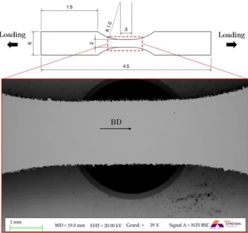
Fully reverse (R =−1) uniaxial tension/compression fatigue tests were conducted in load control using a sinusoidal waveform, in air at room temperature. These tests were conducted on a Zwick resonant testing machine, at 115 Hz using the staircase method, in accordance with the ISO 1099 standard. The stop criterion was a frequency drop of 1 Hz, which corresponds to a fatigue crack of approximately 3 mm in length, or a number of cycles equal to2.1062×106cycles. An infrared camera SC4000 was used during the tests to ensure that there was no self-heating. The geometry of the SLM machined and SLM as-built specimens is givenFig. 2a. The geometry of the HR samples is given
Fig. 2b. Pure torsion tests were performed on SLM HIP machined samples using an electromagnetic BOSE testing machine at 10 Hz. Torsion fatigue tests were conducted under torque control with a load ratio R =−1, in accordance with the ISO 1352 standard. The stop criterion was an exceeding rotation angle of 1 degree which corre-sponds to a fatigue crack of a few mm or a number of cycles equal to
×
2 106cycles. A compressed air cooling system was used to limitate self-heating of the samples. The geometry of the SLM machined samples for torsion tests is shownFig. 2c. Machining specimens (Fig. 2b and c) were used to identify the fatigue crack initiation criterion on smooth specimens. Fatigue tests on as-built specimens (Fig. 2a) are performed to evaluate the effect of surface roughness on HCF strength. In addition to that, tension fatigue tests (R = 0.1) were conducted on SLM as-built (also HIPed) flat specimens on a Zwick resonant testing machine, at 80 Hz. The geometry of the specimens is givenFig. 3. Two faces of the specimens were polished before each fatigue test to observe the crack initiations mechanisms at the surface.
2.3. Strain-imposed cyclic tests
To establish the cycle behavior of the SLM-HIP material, strain-imposed reverse tension cyclic tests were conducted at three different strain levels (0.8%; 1.0%; 1.3%) on a MTS servo-hydraulic testing machine at a f = 0.1 Hz frequency, on standard LCF machined speci-mens. Fig. 4shows the half-life cycle for respectively 0.8%, 1% and 1.3% of imposed strain. Using an optimization procedure, hardening laws were determined in order to correctly describe the experimental cycles. These laws will be used in the elastoplastic numerical simula-tions. The optimized hardening law are rather similar to the
experimental data, except for the slight asymmetry between the tension and compression behavior which is not taken into account.
2.4. Surface analysis
In order to digitize the as-built surfaces,five SLM as-built fatigue specimens were partially scanned using a 3D Bruker Contour GT-K0-X optical profilometer. Four scans in the center of HCF specimens were carried out as shownFig. 2a with a XY resolution of 2μm and a Z re-solution of 8 nm. Each scan measures 5 mm × 1.6 mm. The optical profilometer acquires approximately 80% of the points. The missing
Fig. 1. Microstructure of: HR specimen perpendicular to the Rolling Direction (a); HR specimen parallel to the Rolling Direction (b); SLM HIP specimen at two different magnification (c). Z = Build direction.
Fig. 2. Dimensions of the samples used for Fatigue tests. (a) SLM machined and as-built used for fully reverse uniaxial tension/compression tests. The red rectangle shows the location of the surface scans; (b) HR used for fully reverse uniaxial tension/compression tests; (c) SLM machined specimens used for fully reverse torsion tests. (For interpretation of the references to color in thisfigure legend, the reader is referred to the web version of this article.)
data are restored using a local least-squares method. Since the scanned surface is cylindrical, a flattening step is also applied. It consists of fitting the surface curvature with a quadratic surface of the form
+ + + + + =
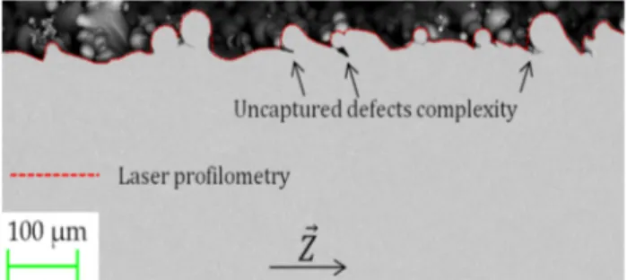
ax2 bxy cy2 dx ey f zand removing this mean surface from the measured data. The result of the procedure is illustrated inFig. 5. One should note that an optical profilometer is unable to fully capture the complexity of additively manufacture surfaces. Indeed, as illu-strated inFig. 6that shows a micrography perpendicular to the surface, additive manufacturing induces a complex morphology that is not fully captured by optical profilometry. In order to assess the effect of this
partial description of the surface, the surface morphology was also acquired by X-ray tomography and both methodology where numeri-cally evaluated. The voxel size is 2.5μm and each scan measures 5 mm × 4.5 mm × 3 mm.
2.5. Numerical simulations
Numerical simulations aims at fully capture the complexity of the local stress-strainfields induced by the surface roughness and to in-troduce them into an HCF strength prediction methodology. The fol-lowing sections describe the meshing and computations procedures and subsequent analysis.
2.5.1. Meshing
Meshed volumes and surfaces are created either from surface mi-crography, surface scans (profilometry) or volume scans (tomography).
•
Meshed surfaces from micrographic analysis: Micrographic ob-servations allow a very accurate surface roughness description. To simulate a real-surface profile, a meshed surface was created using micrographic analysis. The surface was precisely-fitted by using b-spline so that the meshed surface shows a veryfine mesh where the curvature is important. 4 mm long profiles containing 100000 ele-ments with quadratic interpolation were created as shownFig. 7.•
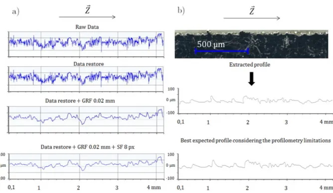
Meshed volumes from profilometric scans: In order to build meshedvolumes suitable for calculation and having a surface morphology matching the as-built surface, the surface data were filtered. A Gaussian Regression Filter (high pass, cutoff: 20μm) and a Statistical Median Filter (range 8 pixels) were applied. Fig. 8a) shows the effects of the filters from raw data to a usable profile. The comparison of a typicalfiltered profileFig. 8a) and a typical profile
obtained from micrography8b) shows that the global aspect of the two profiles are very similar. Since the two extracted profiles were
Fig. 3. Dimensions of the SLM as-builtflat samples used to observe the crack initiation mechanisms occurring during fatigue tests (R = 0.1).
Fig. 4. Experimental and numerical stabilized stress-strain curves of SLM ma-chined specimens at 0.8% 1% and 1.3% of imposed strain.
not generated from the exact same location of the sample they are not supposed to be identical. Each scans is divided into ten surfaces of 0.3 × 0.4 mm and from each surface a meshed volume is gener-ated (0.3 × 0.4 × 0.5 mm). Each volume contains approximately 1 300 000 tetrahedral elements with quadratic interpolation, which ensure the convergence of the mesh. The size of the elements located on the surface is 2μm (side) which corresponds to the XY resolution of the scans (Fig. 9a).
•
Meshed volumes from tomographic scans: The surface of the scanned volume isfirst extracted and smoothed using Aviso soft-ware, a meshed is then generated using Gmsh[31]. The size of theelements located on the surface is 2.5μm which corresponds to the voxel size of the scans. For a cube of 180μm of side, more than 100 000 elements with quadratic interpolation were created (Fig. 9b).
2.5.2. Calculations settings
FE computations were conducted using the FE code Zebulon. Due to the complexity of the surface topology, high local stresses are expected to occur at the surface. In order to evaluate the effect of local plasticity on the near surface stressfields, two different constitutive models were considered: isotropic elasticity and elastoplastic behavior. In the case of elasticity, a Young’s modulus of 110 GPa and Poisson’s ratio of 0.34 were considered. In the case of cyclic plasticity, an Armstrong Frederic
[32]model including two non linear kinematic hardenings and one isotropic hardening was chosen in order tofit experimental data. The yield function is given by:
= − − −
f ( ¯¯, ¯¯ ,σ X R) 3 σ X σ X R
2( ¯¯ ¯¯ ): ( ¯¯ ¯¯ )
d d d d
vm (1)
where σ¯¯dis the deviatoric part of the stress tensor,X¯¯dthe deviatoric
part of the kinematic hardening stress tensor calculated using Eqs.(2) and (3), and R the isotropic hardening calculated using Eq.(4).
Fig. 5. Profilometric data on a cylindrical specimen before and after flattening procedure.
Fig. 6. Micrography of a SLM as-built surface and associated profilometric measurement.
Fig. 7. Micrography of a SLM specimen surface and associated 2D profile.
= − n σ X f ¯¯ 3 2 ¯¯d ¯¯d vm (2) = − m n D CX ¯¯ ¯¯ 3 2 ¯¯ kin (3) = + + R R0 K e( 0 p) (4)
Table 1 summarizes the parameters identified from the experi-mental cyclic behavior obtained from strain-imposed cyclic tests. Using Numerical computations were performed on each meshed volumes to reproduce the experimental fatigue loading (R =−1) ensuring that the nominal maximum axial stress in the computed volume was equal to the nominal cyclic maximum axial stress of HCF tests. In the case of elastoplastic behavior, 2 cycles where sufficient to fully stabilize the local stress strain state. Fig. 10 shows the simulated σ11 stressfield within a volume for an experimental applied nominal maximum stress ofσmax=222.5MPa which corresponds to the fatigue limit of SLM as-built specimens.
2.5.3. Mesoscopic Fatigue Indicator Parameter (FIP)
Since the fatigue loadings considered in this work are relatively simple (tension, torsion loading), even considering the multiaxial stress state induced by the presence of micronotches, the choice of the fatigue criterion is not crucial. Among the possible choices, the Crossland cri-terion was chosen for its simplicity and low computational cost. The local stress-based Crossland criterion[33]is a linear combination of the amplitude of the second invariant of the deviatoric tensor τoct a, and the maximum value of the hydrostatic stress over a cycle σH max, (Eqs.
(5)–(7)). Based on the Crossland criterion a fatigue indicator parameter is proposed as follows:
= +
FIP Mcr( ) τoct a, (M) ασH max, (M) (5) with: = − − ∈ τ (M) 1 S M t S M S M t S M 2max [ ¯¯ ( , ) ¯¯ ( )]: [ ¯¯ ( , ) ¯¯ ( )] oct a t T m m , (6) = ⎡ ⎣ ⎤ ⎦ ∈ σ (M) max 1Trace σ M t 3 ( ¯¯ ( , )) H max t T , (7)
where S M t¯¯ ( , ) is the deviatoric stress tensor and S M¯¯ ( )m the mean
de-viatoric stress tensor. As said previously, the presence of micronotches induces high local stresses and gradients that must be considered to assess the fatigue strength of as-built (rough) parts. In the proposed approach, the gradient effect is taken into account by using a non local FIP consisting in the volumetric averaging of the local FIP at each gauss point of the FE model. The non local FIP, based on the Crossland cri-terion can then be expressed as follows:
〈FIP Mcr( )〉 = 〈τoct a, (M)〉 +α σ〈H max, (M)〉 (8) with:
∭
〈τ M 〉 = V τ M dV ( ) 1 ( ) oct a c V oct a , , c (9)∭
〈σ M〉 = V σ M dV ( ) 1 ( ) H max c V H max , , c (10)whereVc is the averaging volume. In our case,Vcwas considered as a
sphere of radiusDccentred on M, so that:
∫
∫
∫
〈 〉 = =− =+ = = = = τ M πD τ M sinθr drdθdϕ ( ) 1 ( ) oct a c θ π θ π ϕ ϕ π r r D oct a , 4 3 3 0 2 0 , 2 c (11)∫
∫
∫
〈 〉 = =− =+ = = = = σ M πD σ M sinθr drdθdϕ ( ) 1 ( ) H max c θ π θ π ϕ ϕ π r r D H max , 4 3 3 0 2 0 , 2 c (12) This approach was already used by the authors for gradient effect in-duced by pitting in the case of fatigue corrosion[34]and in the case of surface defects induced by a punching process [35]. The fatigue strength is considered to be reached when, at a point M of the con-sidered volume, the following condition is fulfilled:〈FIPcr M〉 =β (13) or when: =〈 〉 = C M FIP β ( ) 1 d cr M (14) where β is a material parameter associated to a given failure probability at a given number of cycles andCdthe danger coefficient.αand β are
Fig. 8. Comparison of a typical surface profile obtained by profilometry (a) to a typical expected surface profile obtained from micrography (b).
material parameters evaluated from two fatigue strengths (tension R =−1 and torsion R = −1 in our case) and at a failure probability of 0.5. The identification of theDccritical distance is presented in Section
2.5.4.
2.5.4. Generalized extreme values distribution
As shown inFig. 10, surface roughness induces a strong hetero-geneity of the local stressfield. The fatigue strength is driven by the most loaded points at the surface of the material, ie the material points
exhibiting the highest FIP orCdparameter. As with previously proposed
methodologies for the statistical evaluation of FIPfield obtained from fulfilled microstructure modeling [30], a generalized extreme values (GEV) statistic framework is proposed to describe the extreme FIP po-pulation of rough surfaces.
For every volume (or surface for 2D calculations), local maximums of the FIP are numerically extracted. As one would expect, they are located at the surface. Extracted material points cannot be closer than 50μm, in order to have approximately one EV per notch. The EV
Fig. 9. Meshed volume generated from a surface scan (profilometry) (a). Meshed volume from volume scan (tomography) (b).
Table 1
Parameters of the elastoplastic model.
Parameter E ν C1 D1 C2 D2 R0 K
distribution being slightly different when extracted from two different volumes, it is not possible to consider each volume as a Representative Volume Element (RVE) from the fatigue point of view. Instead, each volume has to be considered as a Statistical Volume Element (SVE) from which part of the global extreme value data will be obtained. The global EV data set was obtained from the concatenation of EV on each SVE:
•
Between 30 and 40 EV were extracted on each 2D profile and computations were performed on 4 different 2D profiles (143 EV in total).•
Between 15 and 25 EV were extracted on each SVE from profilo-metry and computations were performed on 20 different SVE (451 EV in total).•
Between 8 and 10 EV were extracted on each SVE from tomography and computations were performed on 3 different SVE (32 EV in total).For each condition (2D, profilometry, tomography), the extreme values are gathered and the obtained distribution isfitted using the GEV methods (see[30]for more details on these methods). The median of thefitted distribution will be used in this study to evaluate the HCF strength and will be noted:〈FIPcr p〉=0.5.
Fig. 10. Simulated σ11stressfield within an volume for an experimental applied nominal maximum stress of 222.5 MPa.
Fig. 11. Distribution of the E.V. of the FIP and associated fitted G.E.V.distribution for different critical distances.
Fig. 13. Fracture surface of: an HR machined specimen, 84,749 cycles, 680 MPa (a); a SLM machined specimen, 262,751 cycles, 550 MPa (b); a SLM as-built specimen, 291,965 cycles, 212.5 MPa (c); an SLM as-built specimen, 109,201 cycles, 300 MPa (d).
3. Results and discussions 3.1. HCF tests
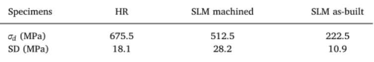
Fig. 12illustrates the fatigue results obtained for uniaxial tension/ compression loading conditions. The HR specimens show the highest fatigue strength, as expected according to the fine equiaxed micro-structure, which is very suitable for fatigue applications [36]. The
reduced fatigue strength of machined SLM specimens compared to HR specimens is due to the change in microstructure (fromfine equiaxed to fully lamellar). The drop in term of maximum stress is about 100 MPa over the total investigated fatigue life range, which corresponds to more than a decade in term of fatigue life. The effect of surface roughness is tremendous since it induces a drop of more than 60% of the fatigue strength (seeTable 2). The difference between the SLM machined and SLM as-built fatigue limit is due to the surface notches which act as
Fig. 14. Observations of surface crack initiation onflat SLM as-built specimens tested in tension (R = 0.1): Main crack and non-propagating cracks.
stress concentrators. One should also note that the machining process most likely generates compression residual stresses[37]but this has not be taken into account in this study.
In addition, fully reversed torsion tests were performed on SLM machined samples in order to determine the fatigue limit which will be used in the numerical simulations. The fatigue limit at2×106cycles determined by the stair case method from 9 specimens is 417 MPa with
an associated standard deviation of 41 MPa.
3.2. Fractography analysis
Authors report that, when the HIP post-processing has not been applied, fatigue cracks in additively manufactured titanium alloys generally initiate from porosities located close to the surface for
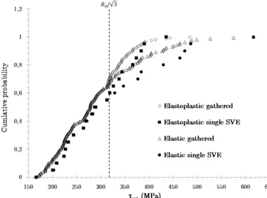
Fig. 16. Cumulative probability function associated to the EV of τoct within an SVE obtained from profilometry for an applied nominal maximum stress
=
σ11 222.5MPa.
machined specimens and from surface defects for as-built specimens, respectively [38]. HIPed and machined specimens initiate from mi-crostructural heterogeneities located at the specimens surface or occa-sionally from sub-surface internal porosities not removed during HIP
[39]. In this study, SEM observations show that fatigue crack initiation sites are always located at the specimens surface. In the case of ma-chined specimens, fatigue crack initiation always occurs from micro-structural heterogeneities located at the specimen surface (Fig. 13a and b), confirming the drastic shrinkage of porosities after HIP process. In the case of as-built specimens, out of 9 broken samples, 7 show a fatigue crack initiation induced by the surface roughness (Fig. 13d) and 2 a
fatigue crack initiation induced by a lack of fusion defect ( area ≈160 μm) remaining at the surface (Fig. 13c). Observations conducted onflat samples tested in fatigue at R = 0.1 show that, after the HCF test at the endurance limit, in addition to a main crack that led to the failure of the specimen, there are also numerous non-propagating cracks measuring between 5 and 10μm initiated from local notch tip. This indicates that the surface is composed of many sharp notches and that a local stress value is sufficient to initiate short fatigue cracks but not to propagate them beyondfirst microstructural barriers, and so not appropriate for direct estimation of the fatigue limit of as-built speci-mens (seeFig. 14).
Fig. 18. Von Mises equivalent stress as a function of the distance from the notch tip for two different notches within an SVE obtained from micrographic analysis and for an applied nominal maximum stressσ11=222.5MPa (a). Von Mises equivalent stress as a function of the distance from the notch tip for 3 SVE, each one associated with a different surface analysis method (b).
3.3. Characterization of the near surface stressfield 3.3.1. Distribution of local values
Whatever the modeling method, surface roughness induces a high number of micronotches. Each micronotch locally modifies the stress field so that stress levels near the notch tip are much higher than the applied nominal maximum stress.Fig. 15shows the distribution of the octahedral shear stress calculated at each Gauss point within a volume obtained from profilometry for an applied nominal maximum stress σ11 of 222.5 MPa for both elastic and elastoplastic computations. Gauss points having a value ofτoct=128MPa are located within the volume sufficiently far from the rough surface to be nonsensitive to the notch effect. Gauss points having a value ofτoctclose to 0 are located within a
bump of the rough surface. It shows that some of the material is in-efficient from a mechanical point of view. The high values ofτoctare
attributed to Gauss points located at the surface, close to micronotches acting as stress concentrators. The difference between elastic and elastoplastic calculations is highlighted for values ofτtoctbeing greater
than R / 30 , which concern less than 0.5% of the Gauss points. Since
plasticity affects the most loaded points, it may significantly modify the EV distribution despite a small impact on the global stress distribution.
Fig. 16illustrates the impact of the constitutive law on the EV dis-tribution ofτoctobtained either from the same SVE or from the gathered
distribution of all SVE. In this SVE, only 9 micronotches induce cyclic plasticity. It means that plasticity is localized in some specific regions at the surface and does not concern all EV locations.
3.3.2. Effect of the volume averaging
Volume averaging over a critical distance is a way to take into ac-count the gradient effect. The larger the stress gradient, the higher the effect of the averaging procedure on the local stress state.Fig. 17shows the probability density function of the EV of τoct extracted from the
same SVE for elastic computations. When averaging, the whole dis-tribution is shifted to lower values and the difference between local and non local values is higher for the high value of the EV. This shows that in this case, higher EV are also associated to higher local stress gradient. Since the plasticity is very local, the averaging procedure drastically reduces the difference between the distribution of EV for elastic and
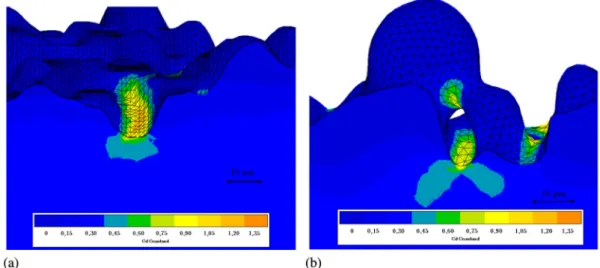
Fig. 19. Cddistribution in the vicinity of a notch within a SVE obtained from profilometric analysis (a) and tomographic analysis (b).
elastoplastic calculations. As shown Fig. 17, the distributions of non local octahedral shear stress are very similar for both calculations, in the HCF regime, so that the choice of the constitutive model will not significantly impact the FIP considered in the HCF criterion.
3.3.3. Gradients at the notch tip
Stress gradients at the notch tip depend on the micronotch geometry which is determined by the surface acquisition procedure (micro-graphy, profilometry or tomography). Fig. 18a shows the Von Mises equivalent stress gradient associated to two different micronotches obtained using micrographic analysis and elastoplastic calculations. Since there are many notch geometries, it is possible to define a Grey zone within which all stress distributions will be contained. The dis-tance affected by the gradient ranges from 10 to 50μm.
The variability of the gradient associated to 2d calculations is also
noticeable in volumes obtained from profilometric and tomographic scans but the highest stress gradients are observed in 2d (Fig. 18b). This is certainly due to thefiltering steps used to build volumes using pro-filometric scans, suitable for calculations.Fig. 18b shows the Von Mises equivalent stress gradient associated to the highest Von Mises value within an SVE obtained by each method. The gradient in SVE obtained from all the methods are rather similar but it can be seen that lower gradient are associated to calculations from profilometric scans. The typical notch root radius associated to SVE obtained from profilometric analysis is bigger which is also a consequence of thefiltering steps.
Fig. 19a and b shows the danger coefficient distribution in the vicinity of a typical micronotch within an SVE obtained respectively from profilometric and tomographic analysis.
The gradient of cumulated plastic deformation per cycle associated the highest plastic deformation value within a SVE is illustratedFig. 20. It shows that the plastic gradient in SVE’s obtained from profilometric and tomographic analysis is very similar whereas the plastic gradient associated with 2d computations is way bigger. Indeed, due to the hardening law associated with our material, d∊
dσ
p
vmbecomes higher when
>
σvm 750MPa so that the small difference regardingσvmbetween 2d
and 3d calculations leads to a huge difference regardingΔ∊p. In the
later condition, the maximum size of the plastic zone is approximately equal to 2μm which corresponds to the critical distance Dc. The
cal-culations using tomographic and profilometric analysis give much lower plasticity levels but the plastic zone associated with the most critical notch within an SVE is the same for all methods.
3.4. GEV and HCF behavior
Fig. 21shows the Crossland diagram associated to a SVE obtained
from micrographic analysis and for an applied mean stress
=
σ11 222.5MPa. Before the averaging procedure, most of the EV are located above the threshold. Based on these values, the loading appears to be very critical regarding fatigue (failure probability> 0.5) even though the applied loading corresponds to the fatigue strength. The averaging procedure brings the highest values closer to the threshold,
Fig. 21. Crossland diagram associated to a SVE obtained from micrographic analysis and for an applied nominal maximum stressσ11=222.5MPa.
Fig. 22. Cumulative probability function of the local and non local FIP dis-tribution for 2d elastic and elastoplastic calculations atσ− =222.5
leading to a more accurate prediction of the criticity of the stress state regarding HCF. The EV (with black borders inFig. 21) are extracted and fitted using the GEV methods. The probability density function asso-ciated to the distribution of EV is shownFig. 22. As presented in Section
2.5.4, the averaging procedure allows to obtain for non local EV a median close to β. Since the plastic zone in the most critical case is approximately the same size as Dc, the median of non local GEV
dis-tribution for elastic and elastoplastic calculations is almost the same as it can be seen Fig. 22. This is valid for an applied mean stress
=
σ11 222.5MPa. When the applied mean stress is higher, the difference between elastic and elastoplastic calculations is more and more
number of cycles. The difference between elastic and elastoplastic computations is noticeable when the applied mean stress is sufficiently high.Fig. 23b shows the result of the methodology for SVE built from tomographic analysis. The simulations give a good estimation of the criticity of the stressfield regarding HCF behavior at ×2 106cycles. However, for higher applied mean stresses, the notch effect is over-estimated. Two main reasons can explain this behavior: the plasticity is not well taken into account. Indeed, the plastic zone being obviously very local, an approach using crystal plasticity calculations should give better evaluation of the stressfield at the notch tip. Current develop-ment aims at addressing this issue which is however outside the scope of this paper. The other reason could be the critical distance which has been calibrated from 2d calculations at2×106cycles and for an applied nominal maximum stressσ− =222.5
d1 MPa. The use of a critical distance
is valid for a given number of cycles[40]and is one way to account for a defect sensitivity defined as: = −
− q K K 1 1 f t where Kf= smooth σ notch σ d d. For a
given material and a given defect it is generally observed that the lower the number of cycles, the lower the difference between smooth σdand
notch σdand so the lower q, meaning that at low number of cycles the
critical distance should be bigger than at high number of cycles. When comparing the predictions for profilometric and tomographic data, an offset of approximately 35 MPa at ×2 106cycles appears between the two data sets which comes from the different descriptions of the sur-faces.
Fig. 23. Master Curve build for SVE obtained from profilometric analysis (a) and tomographic analysis (b).
Fig. 24. Distribution of 〈FIPcr〉within SVE obtained from profilometric analysis.
4. Conclusion
In this study, a methodology accounting for the effect of the surface roughness on HCF strength of Ti-6Al-4V parts obtained by SLM has been developed. The procedure allows estimating the fatigue strength of as-built specimens from which the surface topology has been mea-sured. The differences between elastic and elastoplastic computations regarding the non-local FIP values are very small (at2×106 cycles), which indicates that the methodology is not much sensitive to the hardening law. However, a precise and representative description of the surface is needed in order to correctly take into account the notch effect and to consider a sufficient number of micronotches. The methodology highlighted the fact that measurements from profilometric analysis may not be suitable to predict the fatigue strength of parts obtained by SLM since the micronotches are not well described. One would prefer to-mographic or micrographic measurements, which are able to reproduce faithfully the micronotch morphology associated to the surface. Computations taking into account the residual stresses should extend the validity of the methodology, which should also be challenged for multiaxial loadings. Considering the mechanical behavior as isotropic and homogeneous has to be seen as thefirst statistical momentum of the material behavior. In that sense, the use of an homogeneous behavior is sufficient in a first approximation, even if it will be limitated in terms of local mechanicalfield description. The authors are working on the use of cristal plasticity to evaluate more precisely the impact of local mi-crostructures on the local stress strain state.
References
[1] Do DK, Li P. The effect of laser energy input on the microstructure, physical and mechanical properties of Ti-6Al-4V alloys by selective laser melting. Virtual Phys Prototyp 2016;11(1):41–7.
[2] Gu D, Hagedorn YC, Meiners W, Meng G, Batista RJS, Wissenbach K, et al. Densification behavior, microstructure evolution, and wear performance of selec-tive laser melting processed commercially pure titanium. Acta Mater
2012;60(9):3849–60.
[3] Song B, Dong S, Zhang B, Liao H, Coddet C. Effects of processing parameters on microstructure and mechanical property of selective laser melted Ti6Al4V. Mater Des 2012;35:120–5.
[4] Li P, Warner DH, Fatemi A, Phan N. Critical assessment of the fatigue performance of additively manufactured Ti-6Al-4V and perspective for future research. Int J Fatigue 2016;85:130–43.
[5] Edwards P, Ramulu M. Fatigue performance evaluation of selective laser melted Ti-6Al-4V. Mater Sci Eng, A 2014;598:327–37.
[6] Leuders S, Thöne M, Riemer A, Niendorf T, Tröster T, Richard HA, et al. On the mechanical behaviour of titanium alloy TiAl6V4 manufactured by selective laser melting: fatigue resistance and crack growth performance. Int J Fatigue 2013;48:300–7.
[7] Webster G, Ezeilo A. Residual stress distributions and their influence on fatigue lifetimes. Int J Fatigue 2001;23(Supple):375–83.
[8] James MN, Hughes DJ, Chen Z, Lombard H, Hattingh DG, Asquith D, et al. Residual stresses and fatigue performance. Eng Fail Anal 2007;14(2):384–95.
[9] Van Hooreweder Brecht, Boonen Rene, Moens David, Kruth Jean-Pierre, Sas Paul. On the determination of fatigue properties of Ti6Al4V produced by selective laser melting. 53rd AIAA/ASME/ASCE/AHS/ASC structures, structural dynamics and materials conference. 2012.
[10] Gong H, Rafi K, Gu H, Janaki Ram GD, Starr T, Stucker B. Influence of defects on
mechanical properties of Ti-6Al-4V components produced by selective laser melting and electron beam melting. Mater Des 2015;86:545–54.
[11] Rafi HK, Karthik NV, Gong H, Starr TL, Stucker BE. Microstructures and mechanical properties of Ti6Al4V parts fabricated by selective laser melting and electron beam melting. J Mater Eng Perform 2013;22(December):3872–83.
[12] Atkinson H, Davies S. Fundamental aspects of hot isostatic pressing: an overview. Metall Mater Trans A 2000;31A(December):2981–3000.
[13] Neuber H. Theory of stress concentration for shear-strained prismatical bodies with arbitrary nonlinear stress-strain law. J Appl Mech 1961;28(4):544.
[14] Arola D, Ramulu M. An examination of the effects from surface texture on the strength offiber reinforced plastics. J Compos Mater 1999;33(2):102–23. [15] Arola D, Williams CL. Estimating the fatigue stress concentration factor of machined
surfaces. Int J Fatigue 2002;24(9):923–30.
[16] Peterson. Peterson’s Stress Concentration Factors; 1974.
[17] As S, Skallerud B, Tveiten B. Surface roughness characterization for fatigue life predictions usingfinite element analysis. Int J Fatigue 2008;30:2200–9. [18] Frost NE, Marsh KJ, Pook LP. Metal fatigue. Dover Publications; 1999. 1999-07-07. [19] Smith RA, Miller KJ. Prediction of fatigue regimes in notched components. Int J
Mech Sci 1978;20(4):201–6.
[20] Palin-Luc T, Lasserre S, Berard JY. Experimental investigation on the significance of the conventional endurance limit of a spheroidal graphite cast iron. Fatigue Fract Eng Mater Struct 1998;21(2):191–200.
[21] El Haddad MH, Topper TH, Smith KN. Prediction of non propagating cracks. Eng Fract Mech 1979;11(3):573–84.
[22] Murakami Y, Endo T. Effects of small defects on fatigue strength of metals. Int J Fatigue 1980;2(1):23–30.
[23] Murakami Y, Endo M. Effects of defects, inclusions and inhomogeneities on fatigue strength. Int J Fatigue 1994;16(3):163–82.
[24] Murakami Y. Effect of size and geometry of small defects on the fatigue limit. In: Metal fatigue; 2002. p. 35–55 [Chapter 4].
[25] Taylor D. Geometrical effects in fatigue: a unifying theoretical model. Int J Fatigue 2000;21(5):413–20.
[26] Taylor D. Prediction of fatigue failure location on a component using a critical distance method. Int J Fatigue 2000;22:735–42.
[27] Nadot Y, Billaudeau T. Multiaxial fatigue limit criterion for defective materials. Eng Fract Mech 2006;73(1):112–33.
[28] Morel F, Huyen N. Plasticity and damage heterogeneity in fatigue. Theoret Appl Fract Mech 2008;49:98–127.
[29] Przybyla CP, Mcdowell DL. Simulated microstructure-sensitive extreme value probabilities for high cycle fatigue of duplex Ti 6Al 4V. Int J Plast 2011;27(12):1871–95.
[30] Hor A, Saintier N, Robert C, Palin-Luc T, Morel F. Statistical assessment of multi-axial HCF criteria at the grain scale. Int J Fatigue 2014;67:151–8.
[31] Geuzaine Christophe, Remacle Jean-François. Gmsh: a three-dimensionalfinite element mesh generator with built-in pre-and post-processing facilities. Int J Numer Methods Eng 2009;79(11):1309–31.
[32] Frederick CO, Armstrong PJ. A mathematical representation of the multiaxial Bauschinger effect. Mater High Temp 2007;24(1):1–26.
[33] Crossland B. Effect of large hydrostatic pressures on the torsional fatigue strength of an alloy steel. Proceedings of the international conference on Fatigue of Metals. London: Institution of Mechanical Engineers; 1956. p. 12.
[34] El May M, Saintier N, Palin-Luc T, Devos O. Non-local high cycle fatigue strength criterion for metallic materials with corrosion defects. Fatigue Fract Eng Mater Struct 2015;38(9):1017–25.
[35] Dehmani H, Brugger C, Palin-Luc T, Mareau C, Koechlin S. High cycle fatigue strength assessment methodology considering punching effects. Procedia Eng 2018;213(2017):691–8.
[36] Lütjering G, Williams JC. Titanium. 2nd ed. Springer; 2007.
[37] Matsumoto Y, Hashimoto F, Lahoti G. Surface integrity generated by precision hard turning. CIRP Ann - Manuf Technol 1999;48(1):59–62.
[38] Kasperovich G, Hausmann J. Improvement of fatigue resistance and ductility of TiAl6V4 processed by selective laser melting. J Mater Process Technol 2015;220:202–14.
[39] Chastand V, Tezenas A, Cadoret Y, Quaegebeur P, Maia W, Charkaluk E. Fatigue characterization of Titanium Ti-6Al-4V samples produced by additive manu-facturing. Procedia Struct Integr 2016;2:3168–76.
[40] Yamashita Y, Ueda Y, Kuroki H, Shinozaki M. Fatigue life prediction of small not-ched Ti-6Al-4V specimens using critical distance. Eng Fract Mech