ÉCOLE DE TECHNOLOGIE SUPÉRIEURE UNIVERSITÉ DU QUÉBEC
MANUSCRIPT-BASED THESIS PRESENTED TO ÉCOLE DE TECHNOLOGIE SUPÉRIEURE
IN PARTIAL FULFILLMENT OF THE REQUIREMENTS FOR THE DEGREE OF DOCTORATE IN ENGINEERING
Ph.D.
BY
Patrick BELZILE
ANALYSIS OF SHARED GEOTHERMAL BOREFIELD CONFIGURATIONS
MONTREAL, MAY 26TH 2016
This Creative Commons licence allows readers to dowload this work and share it with others as long as the author is credited. The content of this work may not be modified in any way or used commercially.
BOARD OF EXAMINERS THESIS PH.D. THIS THESIS HAS BEEN EVALUATED BY THE FOLLOWING BOARD OF EXAMINERS
Mr. Louis Lamarche, Thesis Supervisor
Génie mécanique at École de technologie supérieure
Mr. Daniel R. Rousse, Thesis Co-supervisor
Génie mécanique at École de technologie supérieure
Mrs. Claudiane Ouellet-Plamondon, Chair, Board of Examiners
Génie de la production automatisée at École de technologie supérieure
Mr. Christian Masson, Member of the jury
Génie mécanique at École de technologie supérieure
Mr. Radu Zmeureanu, External Examiner Concordia University
THIS THESIS WAS PRESENTED AND DEFENDED
IN THE PRESENCE OF A BOARD OF EXAMINERS AND THE PUBLIC APRIL 26TH 2016
ACKNOWLEDGMENTS
Un plan, ça se change. Lorsque j’ai laissé mon emploi en pétrochimie, le plan était de faire une maîtrise en efficacité énergétique et énergies renouvelables. Un an et demi et je retourne sur le marché du travail. Un cours m’a passionné : Thermique des énergies renouvelables. Le prof passait d’un PowerPoint à Matlab à la vitesse de l’éclair. Pas le temps de cligner des yeux. Le projet demandait beaucoup d’investissement et j’y ai placé tout ce que j’avais. Quand le prof m’a demandé si je voulais faire un doctorat, j’ai refusé. Ça ne faisait pas partie du plan.
Un bon trois mois s’est écoulé avec cette idée qui me chicotte. OK, si je fais un doc, ça va être sur un projet avec du stockage thermique, un projet communautaire. C’est exactement ce que le prof m’a proposé. Merci pour ta patience, ta dévotion et d’avoir partagé ton talent avec moi Louis.
Ça faisait déjà un an que je travaillais avec un gars, du genre rêveur, qui savait partager sa passion. Je ne voulais pas m’en départir. Je lui ai demandé s’il voulait être de la partie et il a accepté. Merci Daniel.
Après un an de travail, je n’avais toujours pas trouvé comment résoudre le problème que Louis m’avait lancé : Les modèles géothermiques sont limités à une seule condition d’entrée pour chaque puits dans un champ. Un cours se donnait à McGill : Computational fluid flow
and heat transfer. Un bon 30 heures de travail par semaine pour un seul cours gradué. C’est
là que le flash est apparu. Thanks for the tackling Rabi Baliga.
Un autre gars n’est jamais été très loin, un gars sage. Le genre de sage qui réfléchit avant chaque mot qu’il prononce. Le genre de gars qui partage sans calculer. Merci Stanislaw.
Il y a une gang avec qui je me suis fait du fun, avec qui j’ai pu discuter de sujets qui n’intéressent pas tout le monde. Merci à toute l’équipe de la Chaire de recherche T3E, en
particulier (par ordre d’apparition) : Guillermo, Nicolas, Messaoud, Geneviève, Laura, Fabien, Pierre-Luc, Frédéric, Jérémie et Kilian.
Je ne peux pas toujours discuter de mes problèmes techniques avec ma famille, ça les ennuierait plus que ça m’aiderait. Néanmoins, ils ont toujours été là pour partager avec moi le meilleur et le pire. Merci meman, pepa, frèrot, « chacha » de belle-sœur, Normand, petit Olivier qui grandit très vite et mini Juliette qui a fait fondre mon cœur à première vue. Merci, je vous aime.
À mes amis, surtout ceux qui me répétaient régulièrement : « C’est pas encore fini ça? », surtout quand les temps étaient durs. Merci pour les « encouragements », vous vous reconnaîtrez.
Un plan, ça se change. Maintenant rendu à la croisée des chemins, je ne vois que des opportunités d’apprendre, de me relever, de rire et de continuer de rêver. Merci la vie.
ANALYSIS OF SHARED GEOTHERMAL BOREFIELD CONFIGURATIONS Patrick BELZILE
ABSTRACT
Geothermal systems have been used in ground source heat pumps applications for decades. They are gaining in interest in recent years through community and hybrid systems. Inconveniently, nearly all of the available geothermal borehole models are limited to the same inlet condition for each U-tubes and geothermal borefields models to the same inlet condition for each borehole. This research project proposes models and applications to shared and hybrid geothermal systems, in residential/solar application. The aim of the project is to improve the efficiency of heat transfer and storage of shared and hybrid geothermal boreholes and borefields by segregating their inlet conditions.
The approach used in this research project can be divided in three parts: the ground model, the single U-tube model and double U-tube model. The ground model is a 2D diffusion Control Volume Finite Difference Method (CVFDM) model. The single U-tube fluid-to-ground analytical model is based on delta thermal resistance analogy, adding a resistance outside the borehole for the shape factor. The double U-tube model is an addition to an existing model that considers the angle, distance and flow direction of the U-tubes legs. It also considers different mass flowrate and specific heat of the fluid in each U-tube.
In the applications, the heat pumps of 12 residential buildings circuit and 24 m2 of solar collectors per residential building circuit were coupled to different borehole and borefield configurations. Three main categories of configurations are: a mitigating loop mixing fluids uphill to the borefield, segregating the circuits in different boreholes in a borefield (independent boreholes) and in circuits of double U-tubes boreholes (independent circuits). The energy consumption of each heat pump over the three years period was 10 884 kWh for the base case without solar collectors. The mitigated loop saved 2.4%, as for the independent boreholes central configuration with 4.5 m and the staggered configuration with 3 m and 4.5 m. The independent circuit gave the best results with 6.4% savings for the 12 borehole heat exchangers case and 9.3% for the 24 borehole heat exchangers.
Keywords: Geothermal borefield model, Shared borefield, Hybrid Geothermal, Ground source heat pump
ANALYSE DE CONFIGURATIONS DE CHAMPS GÉOTHERMIQUES PARTAGÉS Patrick BELZILE
RÉSUMÉ
Les systèmes géothermiques sont utilisés dans des applications de pompes à chaleur depuis des décennies. Les systèmes communautaires et hybrides gagnent en popularité depuis quelques années. Malencontreusement, presque tous les modèles de puits géothermiques disponibles sont limités à une seule condition d'entrée pour chaque tube en U et les modèles de champs géothermiques à la même condition d'entrée pour chaque puits. Ce projet de recherche propose des modèles et applications aux systèmes partagés et hybrides géothermiques dans des applications résidentielles/solaires. Le but du projet est d'améliorer l'efficacité du transfert de chaleur et de stockage des puits et champs géothermiques partagés et hybrides en séparant leurs conditions d'admission.
L'approche utilisée dans ce projet de recherche peut être divisée en trois parties: le modèle de sol, le modèle de simple tube en U et modèle de double tube en U. Le modèle du sol utilise une méthode de différences finies (CVFDM) en 2D et diffusion seulement. Le modèle analytique fluide-sol de simple tube en U est basé sur l’analogie de résistance thermique en delta, en ajoutant une résistance à l'extérieur du puits pour tenir compte d’un facteur de forme. Le modèle à double tubes en U est un ajout à un modèle existant qui considère l’angle, la distance entre les jambes des tubes en U, ainsi que le sens de l’écoulement. Le débit de massique et la chaleur spécifique du fluide peuvent être définis indépendamment dans chaque tube en U.
Dans les applications, le circuit de pompes à chaleur de 12 bâtiments résidentiels et le circuit de 24 m2 de capteurs solaires par résidence ont été couplés à des configurations de puits géothermiques et de champs de puits différents. Trois principales catégories de configurations sont simulées: une boucle mitigée qui mélange les fluides de circuits en amont du champ de puits, une ségrégation des circuits dans différents puits dans un champ (puits indépendants) et la ségrégation des circuits dans chaque tube en U de doubles tubes en U (circuits indépendants). La consommation d'énergie de chaque pompe à chaleur sur de trois ans était 10 884 kWh pour le cas de base sans capteurs solaires. La boucle mitigée a économisé 2,4%, tout comme pour les forages indépendants en configuration centrale avec 4,5 m et les configurations en quinconce de 3 m et 4,5 m. Le circuit indépendant a donné les meilleurs résultats avec 6,4% d'économies pour le cas 16 puits et 9,3% pour le 24 puits. Mots-clés: modèle de champ de puits géothermiques, champ de puits partagés, géothermie hybride, Pompe à chaleur géothermique
TABLE OF CONTENTS
Page
INTRODUCTION ...1
0.1 Context ...1
0.2 Objectives and methodology ...2
0.3 Thesis content ...3
CHAPTER 1 LITTERATURE REVIEW ...5
1.1 Ground-source heat pump ...6
1.2 Ground temperature ...9
1.3 Ground Heat Exchange ...11
1.3.1 Boreholes thermal resistance ... 13
1.3.2 Ground models ... 15
1.3.3 Configurations... 20
1.3.4 Control strategy ... 21
1.4 Sizing geothermal loops ...22
1.5 Software ...24
CHAPTER 2 SEMI-ANALYTICAL MODEL FOR GEOTHERMAL BOREFIELDS WITH INDEPENDENT INLET CONDITIONS ...27
2.1 Abstract ...27
2.2 Introduction ...27
2.3 Brief literature review ...28
2.4 Description of the proposed model ...31
2.4.1 Numerical part ... 31
2.4.2 Analytical part ... 32
2.4.3 Potential of the proposed model ... 39
2.5 Validation ...41
2.5.1 A first validation of the 2D solver ... 41
2.5.2 The determination of the appropriate grid size ... 43
2.5.3 Comparison with the DST method for steady inlet temperature ... 46
2.5.4 Comparison with the DST method for unsteady inlet temperature ... 47
2.6 Application example with variable inlet temperatures ...48
2.7 Results ...51
2.8 Conclusion ...56
CHAPTER 3 GEOTHERMAL HEAT EXCHANGE IN BOREHOLES WITH INDEPENDENT SOURCES ...59
3.1 Abstract ...59
3.2 Introduction ...60
3.3 Original symmetric double U-tube configuration ...62
3.4 New non-symmetric double U-tube configuration ...66
3.6 Applications ...72
3.7 TRNSYS Model ...76
3.8 Symmetric double U-tubes ...78
3.9 Non-symmetric double U-tubes ...81
3.10 Conclusion ...84
CHAPTER 4 HYBRID RESIDENTIAL SOLAR GEOTHERMAL BOREFIELD CONFIGURATIONS ...87
4.1 Abstract ...87
4.2 Introduction ...88
4.3 Base configuration ...90
4.3.1 Base case simulation ... 92
4.4 Mitigated loop ...94
4.5 Independent boreholes ...97
4.5.1 Central configuration ... 98
4.5.2 Staggered configuration ... 100
4.6 Independent circuits ...100
4.6.1 Symmetric double U-tubes ... 101
4.6.2 Non-symmetric double U-tubes ... 102
4.7 Comparison of configurations...103
4.7.1 Ground heat balance ... 104
4.7.2 Borefields outlet fluid temperatures ... 106
4.7.3 Heat pumps energy consumption ... 107
4.8 Conclusion ...110
CONCLUSION ...113
APPENDIX I INDEPENDENT CIRCUIT MODEL COEFFICIENTS ...117
APPENDIX II RESIDENTIAL/SOLAR APPLICATIONS RESULTS ...121
LIST OF TABLES
Page
Table 1-1 Discontinuous operation heat transfer rate increase ...21
Table 2-1 Richardson’s Extrapolation ...45
Table 2-2 Typical geothermal parameters ...49
Table 2-3 Simulation results comparison [kWh] ...55
Table 2-4 Geothermal outlet fluid temperature comparison ...55
Table 2-5 Energy consumption comparison [kWh] ...55
Table 3-1 Simulation parameters ...74
Table 3-2 Total energy balance ...76
Table 3-3 Energy balance [MWh] ...76
Table 3-4 Typical geothermal parameters ...78
Table 3-5 Simulation results for the two configurations: Heat extracted and injected by the heat pump, heat provided by the solar collectors and energy balance [kWh] ...84
Table 3-6 Energy consumption comparison using simulation results for the two configurations [kWh] ...84
Table 4-1 Typical geothermal parameters ...92
Table 4-2 Geothermal outlet fluid temperature comparison for 16 BHE (heat pump circuit) ...106
Table 4-3 Geothermal outlet fluid temperature comparison for 24 BHE (heat pump circuit) ...107
LIST OF FIGURES
Page
Figure 1-1 Thermal storage processes ...5
Figure 1-2 Ground-source heat pump (Kavanaugh, 1985) ...7
Figure 1-3 Heat pump COP vs. EWT ...8
Figure 1-4 Ottawa ground temperature profile ...9
Figure 1-5 Energy balance on ground (Florides and Kalogirou, 2007) ...10
Figure 1-6 Schematic of a section of a vertical borehole ...11
Figure 1-7 Heat transfer of BTES ...12
Figure 1-8 Thermal resistance of a borehole heat exchanger ...13
Figure 1-9 Schematic representation of interference between boreholes (Hellström, 1991) ...19
Figure 1-10 Hybrid system (Yavuzturk and Spitler, 2000) ...22
Figure 1-11 Simulation programs comparison (Shonder and Hughes, 1998) ...24
Figure 2-1 Shape factor ...33
Figure 2-2 Combined borehole and shape factor thermal resistance analogy ...34
Figure 2-3 Ground temperature surrounding a source term ...35
Figure 2-4 Proposed model ground temperature, 4x4 borefield, 1 year simulation ....40
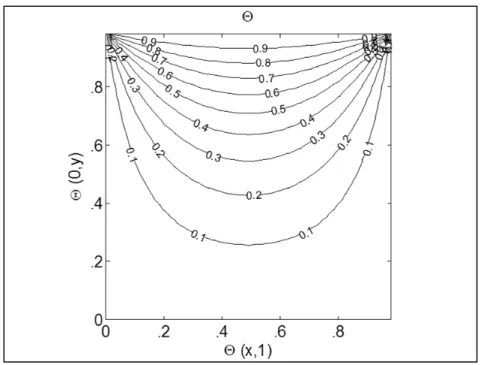
Figure 2-5 Analytical solution of 2-D steady homogeneous heat conduction without source, θ(x,1)=1, θ =0, elsewhere ...42
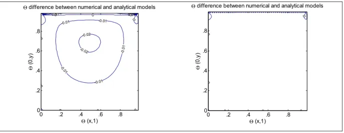
Figure 2-6 Discrepancy between the numerical and analytical solutions: Control-volumes (CV) per axis: left-51 ; and right-101. ...43
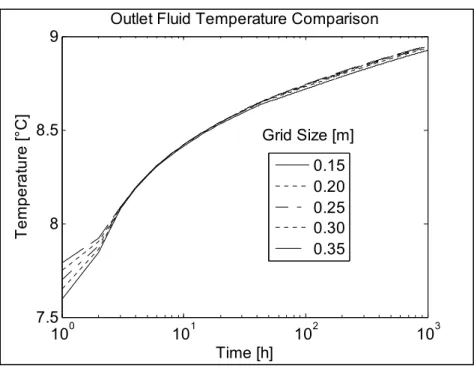
Figure 2-7 Variation of the outlet fluid temperature with time for selected values of the grid size ...44
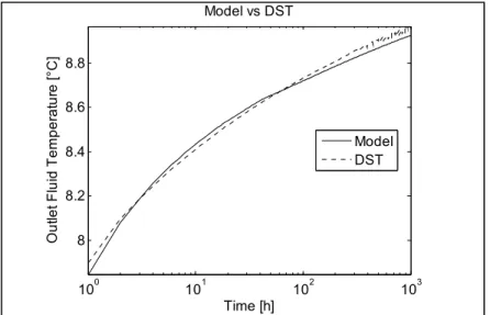
Figure 2-9 Comparison of the DST and proposed model for the predictions of the outlet fluid temperature with time: one borehole, steady inlet
temperature ... 46
Figure 2-10 Comparison of the DST and proposed model for the predictions of the outlet fluid temperature with time: 3x3 borehole, unsteady inlet temperature ... 47
Figure 2-11 Residential loads (left) and heat pump power (right) ... 48
Figure 2-12 Schematic of a single-loop geothermal borefield with inline collectors and a 4x4 borehole arrangement... 50
Figure 2-13 Schematic of an independent borehole geothermalborefield with central connected solar collectors and a 4 x 6 borehole arrangement ... 51
Figure 2-14 Single-loop 4x 4 configuration outlet fluid temperature predictions of the geothermal heat pump: (left) after one year; (right) after 5 years of operation ... 52
Figure 2-15 Independent borehole central 4 x 6 configuration outlet fluid temperature predictions for the geothermal heat pump: (left) after one year; (right) after 5 years of operation ... 53
Figure 2-16 Independent boreholes central configuration ground temperature profile ... 54
Figure 2-17 Heat pump energy consumption ... 56
Figure 3-1 Independent borehole arrangement: X, solar supplied heat; O, extracted heat ... 61
Figure 3-2 Double U-tube geothermal system ... 63
Figure 3-3 Heat flow patterns of two U-tubes in a borehole: 2, 3-4; 3, 2-4; 1-2, 4-3. ... 63
Figure 3-4 Non-symmetric configuration ... 67
Figure 3-5 Temperature profiles, cold leg left, hot leg right ... 70
Figure 3-6 Solution comparison, cold leg left, hot leg right ... 72
Figure 3-7 Application configuration ... 73
Figure 3-9 EWT of the heat pump 2 ...75
Figure 3-10 Residential thermal and heat pump energy ...77
Figure 3-11 Schematic of the system involving one heat pump, one collector area and a symmetric configuration for the borefield ...79
Figure 3-12 Geothermal borehole thermal loads ...80
Figure 3-13 Symmetric configuration heat pump circuit borefield outlet fluid temperature with respect to time: (left) after one year; (right) after 5 years of operation ...81
Figure 3-14 Schematic of the system involving one heat pump,one collector area and a non-symmetric configuration for the borefield. ...82
Figure 3-15 Non-symmetric configuration heat pump circuit borefield outlet fluid temperature with respect to time: (left) after one year; (right) after 5 years of operation ...83
Figure 4-1 Base configuration ...90
Figure 4-2 Residential thermal loads ...91
Figure 4-3 Geothermal Outlet Fluid Temperature Base Case 3x4 Borefield ...93
Figure 4-4 Mitigated loop configuration ...94
Figure 4-5 Single-loop 3x4 configuration outlet fluid temperature predictions of the geothermal heat pump: No sum strategy; (left) after one year; (right) after 3 years of operation ...95
Figure 4-6 Mitigated loop heat pump energy balance ...96
Figure 4-7 Mitigated loop ground energy balance ...97
Figure 4-8 Independent boreholes, central configuration ...98
Figure 4-9 Independent Boreholes Central Configuration Ground Temperature Profile ...99
Figure 4-10 Independent boreholes, staggered configuration ...100
Figure 4-11 Independent circuit, symmetric configuration, Type C ...101
Figure 4-13 Independent circuit non-symmetric configuration heat pump circuit borefield outlet fluid temperature ... 103 Figure 4-14 Ground heat balance for all simulations involving 3x4 borefields ... 104 Figure 4-15 Ground heat balance for all simulations involving4x6 borefields ... 105 Figure 4-16 Heat pump energy consumption for all simulations involving 3x4
borefields ... 108 Figure 4-17 Heat pump energy consumption for all simulations involving 4x6
LIST OF ABREVIATIONS BHE Borehole Heat Exchanger
BTES Borehole Thermal Energy Storage COP Coefficient Of Performance CPU Central Processing Unit
CV Control Volume
CVFDM Control Volume Finite Difference Method CVFEM Control Volume Finite Element Method DST Duct Storage System
ÉTS École de technologie supérieure
EWT Heat Pump Entering Water Temperature GCHP Ground Coupled Heat Pump
GHC Grant-Harvey Center
GSHP Ground Source Heat Pump
HVAC Heating, Venting and Air-Conditioning IPCC Intergovernmental Panel on Climate Changes MLAA Multiple Load Aggregation Algorithm
RMS Root-Mean-Square
SBM Superposition Borehole Method TDMA Tri-Diagonal Matrix Algorithm
TRT Thermal Response Test
LIST OF SYMBOLS AND UNITS OF MEASUREMENTS Chapter 1
Kusuda model
A annual average earth temperature [°F]
BO projected earth surface temperature amplitude (B at x=0) [°F]
D thermal diffusivity [ft2/hr]
PO projected phase angle at the earth's surface (x=0) [rad]
T period of the temperature cycle (8766 hrs) [hr]
x downward distance coordinate from the earth's surface depth [ft]
ϴ elapsed time from January 1st, 1sthour [hr]
Chapter 2
c Specific heat (J kg-1 K-1)
D Borehole diameter used in shape factor definition (m)
dx Control volume dimension in the x-direction (m)
dy Control volume dimension in the y-direction (m) Fo Fourier number
Fr Fraction of propylene-glycol in water inter Between boreholes (m)
L Length (m)
k Thermal conductivity (W m-1 K-1) Mass flow rate (kg m-3)
q Heat extraction/injection rate (W)
R Thermal resistance (m K W-1)
r Radius (m)
Rc Shape factor equivalent thermal resistance (m K W-1)
S Shape factor between borehole and control volume boundaries
ST Source term
undist Undisturbed
V Volume (m3)
W Control volume width used in shape factor definition (m)
z Non-dimensional thermal resistance factor Greek letters
λ Ground thermal conductivity (Eskilson)
ρ Density or specific weight Subscripts
1 Refers to the branch of the fluid flowing downward in the borehole 2 Refers to the branch of the fluid flowing upward in the borehole a Average
a related to the thermal resistance between the two pipes of the borehole b Borehole
c related to the thermal resistance between the borehole and its control-volume f Fluid g Grout s Ground tot Total in inlet out outlet
n,s,e,w North, South, East, West neighbors of node i,j ne, se, nw, sw North-east, South-east, North-west, South-west Superscripts
‘ Per unit length * Effective
Chapter 3
k thermal conductivity (W m−1K−1) cp Fluid specific heat (J kg-1 K-1)
mass flow rate (kg s−1)
q′ heat flux per unit length (W m−1) r radius (m)
xc half shank spacing (m)
T temperature (°C)
x,y,z spatial Cartesian coordinates (m)
xo,yo,zo coordinates of the entrance of the borehole (m)
d diameter (m)
Di Pipe inner diameter (m)
Do Pipe outer diameter (m)
G
h heat transfer coefficient, (W m−2K−1) Tfi1 Fluid inlet temperature, circuit 1 (°C) Tfi2 Fluid inlet temperature, circuit 2 (°C) L Borehole depth (m)
R Borehole thermal resistance (W m-1 K-1) S modified thermal resistances
Z dimensionless depth
Greek letters
αs soil thermal diffusivity (m2 s–1) α mass flow ratio
ß angle of rotation (deg)
ε efficiency
χ twice the dimensionless borehole depth (Eq. 23)
θ non-dimensional temperature
Subscripts
b borehole f mean fluid
g grout hp heat pump o far-field p pipe s soil i image in inlet Superscripts
R with respect to the reference frame (Fig. 1)
b with respect to the borehole frame o new resistances
’ per unit length
~ dimensionless variable
^ dimensionless variable
_ mean value
INTRODUCTION
0.1 Context
Ground source heat pumps or low temperature geothermal systems, are used in heating and cooling applications; mainly buildings. Boreholes are drilled into the ground to depths that can reach 600 m and in closed-loop systems, U-tubes are inserted in them. Thus, a heat transfer fluid exchanges heat between heat pumps and the surrounding ground. Low temperature geothermal systems are known for their great efficiency provided by the interesting coefficient of performance (COP) of their heat pumps, but also for their high capital investment mainly caused by drilling depth costs. The Intergovernmental Panel on Climate Changes (IPCC) projects that the heat energy produced by ground source heat pumps will evolve from 0.4 EJ/year in 2010 to 7.2 EJ/year in 2050 (Goldstein and al., 2011).
In many parts if the globe, buildings annual thermal loads are unbalanced between heating and cooling. In cold climates, more heat is extracted from the ground during heating period than injected during its cooling counterpart. This is prone to make the ground colder every year and after a certain period of time, could make the geothermal system unusable. Moreover, if the ground freezes, the boreholes could be permanently damaged. Hybrid systems are then a prospective solution for such an issue.
It is becoming more common to see shared and hybrid geothermal borefields. Many buildings and processes with different heating and cooling loads profiles can share the same geothermal loop. It is possible, sometimes even mostly desirable, to couple complementary load profiles. An example of hybrid geothermal system would be to couple solar thermal collectors with heat pumps to the geothermal loop. Geothermal systems can also be coupled to cooling towers and waste heat from industrial processes. The University of Wisconsin found economic and environmental advantages to hybrid geothermal systems compared to classic by reducing the rate of return on investment and the CO2 emissions (Hackel and Pertzborn, 2011c).
Existing installations of hybrid geothermal systems can be found in Canada. The Drake Landing Solar Community, in Alberta, is composed of 56 residential buildings and a solar collectors loop sharing the same geothermal borefield. The University of Ontario Institute of Technology installed a 384 boreholes borefield to heat and cool 8 of the campus buildings.
In the United States of America, the Ball State University is coupling 47 buildings through a 3 600 boreholes borefield. In 2005, there were about 600 000 ground source heat pumps installed in the USA and 200 000 in Sweden, which is more than 1% of the buildings in the latter case (Curtis and al., 2005).
0.2 Objectives and methodology
Nearly all available geothermal mathematical models consider only one inlet condition for all of the U-tubes and boreholes of a borefield, limiting the amount of possible configurations and control strategies to be simulated and then evaluated.
The objective of this research is to improve the efficiency of shared and hybrid geothermal systems by segregating heat transfer sources. This will be achieved by:
• developing a semi-analytical model that considers independent inlet conditions for each borehole of a borefield in the first part;
• developing a model that considers independent circuits of double U-tubes in each borehole in the second part.
The ground is modeled as a 2D control volume finite difference method (CVFDM). The 3D effect is found after long periods of time with largely imbalanced loads and one objective of this work is to balance the loads, so a 2D model is deemed acceptable for now. Only diffusion of heat is considered for now. Since the boreholes are circular and the control volumes regular and uniform (square), an analytical shape factor is used at the source term control volumes. This part of the model describes the heat transferred between the external
ground and the borehole wall. An analytical model based on thermal resistances is used to describe the heat transferred between the internal fluid and the borehole wall.
A second model is developed to describe the behavior of a double U-tube borehole where the two legs of the U-tubes are coupled to different sources. It is a complement of an existing model (Eslami-Nejad and Bernier, 2011b), in addition of having different capacitances in each leg. This model uses the above-mentioned ground-to-borehole wall model.
0.3 Thesis content
This thesis is divided into four chapters:
1. The first chapter presents a general literature review on low temperature geothermal systems. Main subjects studied were ground source heat pumps, ground models, borehole thermal resistance, configurations, control strategies and sizing of ground source heat pump systems.
2. The second chapter is a paper published in Geothermics on a semi-analytical model that can describe the behavior of geothermal borefields with independent inlet conditions in each borehole. The ground is modeled as a 2D control volume finite difference method. An analytical model is used to describe the heat transfer between the borehole wall and the heat transfer fluid. A shape factor is used to couple the circular borehole to a square control volume. An application of residential/solar hybrid ground source heat pump system is presented where boreholes in the center of a borefield are coupled to solar collectors and the outer boreholes to residential heat pumps.
3. The third chapter is a paper published in Applied Thermal Engineering describing a model where legs of double U-tubes can have different inlet conditions. The model is based on a previous paper (Eslami-Nejad and Bernier, 2011b), that allows to model
double U-tubes with different angles between the legs, but the proposed model also allows the flowrate and the capacitance of the fluid to be different in each leg. Application examples include two heat pumps coupled to different circuits and a residential/solar application, coupling solar collectors to one circuit and residential heat pumps to the other.
4. The fourth chapter is a paper yet to be accepted in Renewable Energy. It presents residential heat pumps and solar applications simulations using the previous models. The objective is to compare the performances of different configurations of hybrid ground source heat pump systems. A base case without solar collectors is compared to a classical mitigated loop configuration. Using the both previously developed models, independent boreholes and independent circuits configurations are also simulated.
This thesis ends with a general conclusion on the three papers, highlighting the advantages and inconvenient of each configuration and recommending further work that could be done.
CHAPTER 1
LITTERATURE REVIEW
Energy can be found in numerous states such as mechanical, electrical, chemical and thermal. Thermal energy can be stored with different methods which can be divided in two main categories: sensible and latent heat storage. Sensible heat storage uses a material’s temperature difference to store energy while latent heat storage uses the energy required to change the phase of a material. Even though latent heat storage is usually more compact than sensible heat storage for the same amount of energy stored, there are technical difficulties to implement it such as supercooling, the fact that a heat exchanger that can deal with two phases is hard to build and there is irreversibility in the process (Dinçer and Rosen, 2011).
Generally, thermal storage is divided in three processes: recharge, storage and discharge, as shown in Figure 1-1.
Figure 1-1 Thermal storage processes
The ground can be used as a sensible heat storage medium. Ground heat storage, also known as underground thermal energy storage (UTES), is divided in four main categories (Pahud, 2002): Discharge Re ch ar ge Storage
• Ground diffusive storage, which uses the ground as storage medium and is normally a vertical heat exchanger. Borehole thermal energy storage (BTES) is one type of exchanger;
• Earth storage, which also uses the ground as a storage medium, but is normally horizontal, such as an excavated volume. The top surface can be insulated;
• Aquifer storage that uses underground water and its surrounding ground as storage medium;
• Water storage that can be underground or above ground tanks, insulated or not.
This research deals with shared geothermal fields between different sources. It is divided in major themes: Ground-source heat pump, ground temperature, ground heat exchange, sizing geothermal loops and software.
1.1 Ground-source heat pump
The main utilization of geothermal boreholes and borefields is the coupling with a heat pump, called ground source heat pump or ground coupled heat pump. Heat pumps require low-temperature heat sources, such as ambient air, groundwater and ground. In some locations, air temperature can be too low to extract any heat from it. Groundwater, in sufficient quantities, is an interesting alternative, but is not available everywhere. The ground however, does not involve these limitations.
Figure 1-2 Ground-source heat pump (Kavanaugh, 1985)
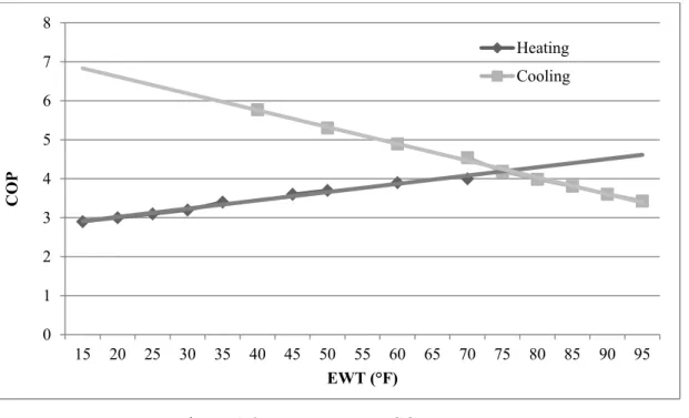
Ground-source heat pumps (GSHP) or ground-coupled heat pumps (GCHP) shown in Figure 1-2 are systems that circulate water, or a mixture of water and anti-freeze, in a closed-loop circuit. They can be horizontal or vertical. The coupling to a heat pump permits using the ground as a heat sink (condenser) or a heat source (evaporator) for cooling or heating purpose, respectively. In heating mode, the efficiency of the system increases as the entering water temperature (EWT) rises. The efficiency reduces with time if the annual balance is towards heat extraction from the ground. The same efficiency reduction can be observed in cooling mode when the EWT rises. The COP is the ratio of supplied heat to the supplied work consumed by the heat pump. Figure 1-3 represents an example of coefficient of performance (COP) as a function of EWT.
Figure 1-3 Heat pump COP vs. EWT
Each heat pump has its own specifications for minimum and maximum EWT. AHRI/ASHRAE/ISO 13256-1 code (ANSI/ARI/ASHRAE/ISO, 2005) tests heat pumps performances with heating EWT at 0°C (32°F) and cooling EWT at 25°C (77°F), but some can operate between -6°C (21°F) and 48°C (118°F). This heat pump EWT is in fact the leaving water temperature from the borehole, so the design of the BTES should be within the heat pump boundaries.
The other side of the heat pump is the heating and cooling demand, usually from a building. The heat pump can exchange heat with the air, radiant floor water or even domestic hot water. To achieve this, some components are required such as circulation pumps, heat exchangers, compressor, expansion valve and/or a fan. The building heating, ventilation and air-conditioning (HVAC) demand will size the heat pump capacity.
The impact of the on/off cycle of ground-source heat pumps using steady-state models leads to overestimation of energy use and to a different design that would have been done with
0 1 2 3 4 5 6 7 8 15 20 25 30 35 40 45 50 55 60 65 70 75 80 85 90 95 COP EWT (°F) Heating Cooling
dynamic models (Kummert and Bernier, 2008). Therefore, the dimensions of the borefields depend greatly on the assumptions made during the design.
1.2 Ground temperature
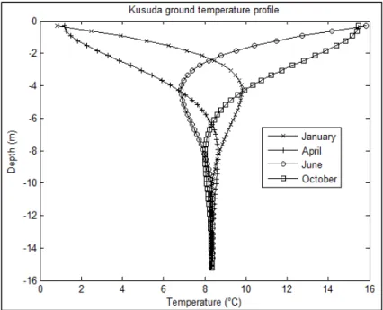
Kusuda provides surface temperature profiles as simple harmonic presentation, which are considered by the authors as a “fair approximation of monthly average earth temperature except near the surface, provided the annual average temperature, the annual amplitude and phase angle of the surface temperature, and the thermal diffusivity are known.” (Kusuda and al., 1965). Kusuda model is used in TRNSYS® and TESS® components. The model is presented in equation 1.1. 2 exp DT xcos T A BO x PO T DT π πθ π − = − − − (1.1)
Figure 1-4 shows ground temperature profile using Kusuda supplied parameters for Ottawa, Ont. (Canada): A = 47.0°F, B0 = 21.0°F, P0 = 0.64, D = 0.025.
This model shows that seasonal weather impacts are limited in depth in the ground. Temperature stabilizes around 15 m deep to 8.3°C (47°F). Mihalakakou developed a surface ground temperature model based on many factors such as convective energy exchange between air and soil, solar radiation absorbed, evaporation and long-wave radiations emission (Mihalakakou and al., 1997). Figure 1-5 represents these factors.
Figure 1-5 Energy balance on ground (Florides and Kalogirou, 2007)
Near the surface (0 - 10 m), heat is exchanged with the environment (sun, evaporation, ambient air, etc.). At mid-distance, fewer variations can be observed (10 m - 20 m). Deeper than 20 m, very low variations are observed. Energy transferred from the Earth’s core gives a geothermal gradient of about 15 to 35 °C/km in the United States (Nathenson and Guffanti, 1988). Depending on the depth considered for thermal storage, the weather conditions might not always have a significant impact on it; such could be the case for BTES.
A more recent study based on energy balance of the ground surface takes into consideration convection from the wind, solar energy, sky temperature and water evaporation factors has shown good agreement with experimental results (Badache and al., 2016).
1.3 Ground Heat Exchange
The BTES method is normally found in the form of a vertical U-tube heat exchanger buried in the soil. It is composed of a plastic pipe, inserted in a vertically drilled borehole which is can be filled with grout as schematically shown in Figure 1-6.
Figure 1-6 Schematic of a section of a vertical borehole
To ensure heat transfer to and/or from the ground, a heat transfer fluid is circulated through the plastic tube. Convective heat transfer occurs between the fluid and the inner surface of the plastic tube and conductive heat transfer occurs through the plastic pipe from the inner to the outer surface. There is a contact resistance between the tube and the grout. Then, heat is diffusing across this resistance and the grout. This whole portion of heat transfer is modeled herein as an equivalent borehole thermal resistance that accounts for the four phenomena. However, the contact resistance is found to be negligible and is not considered herein. The
outer part, composed of conductive heat transfer from the borehole to the ground and convective heat transfer from groundwater to the borehole, is called ground heat exchanger.
Figure 1-7 Heat transfer of BTES
The impact of groundwater flow on geothermal borefields has been studied and models are available (Bauer and al., 2009; Chiasson, 1999; Lee and Lam, 2007; Molina-Giraldo and al., 2011; Niibori and al., 2005; Sutton and al., 2003; Wang and al., 2009). The axial effect and groundwater flow is recommended to be taken into considerations with Peclet numbers between 1.2 and 10 (Molina-Giraldo and al., 2011). Nevertheless, the present research will not take groundwater flow into consideration.
For most of the available studies, the approach to model a BTES system considers heat transferred between:
• the fluid and the inside of the pipe;
q
conv,fluidq
cond,groundq
cond,borehole• the inside of the pipe and the outside of the borehole; • the outside of the borehole and the ground;
This framework will be adopted in this study.
1.3.1 Boreholes thermal resistance
In order to evaluate the heat transferred from the borehole surface to the fluid, the thermal resistance approach can be used. The heat transfer per unit length, subject to the above-mentioned assumptions, through all components (q’b) is represented in eq. (1.2). It can be
modeled as thermal resistances as shown in eq. (1.3) (Incropera and DeWitt, 2007) and represented in Figure 1-8. ' ' b f b b T −T =q R (1.2) , , 'b 'conv f 'cond p 'g R = R +R +R (1.3)
Figure 1-8 Thermal resistance of a borehole heat exchanger
Tf Tp Tb
The heat from the source is exchanged with the fluid. This source can be steady or unsteady. The heat is then transferred to the surface of the U-tube based on eqs. (1.4) and (1.5) (Incropera and DeWitt, 2007).
,
conv f p
q =hA TΔ (1.4)
Here, ΔT is the temperature difference between surfaces and h is the convection heat transfer coefficient. Since there are two pipe sections per U-tube, the convection resistance per unit length can be divided by 2,
, 1 ' 4 conv f pi R r h π = (1.5)
where rpi is the internal radius of the pipe. The second resistance is between the inside of the pipe and the grout (R’cond,p),
(
)
, ln / ' 4 po pi cond p p r r R k π = (1.6)where kp is the thermal conductivity of the pipe.
Many models are available to evaluate the borehole thermal resistance (R’g) :
• Paul (Paul, 1996);
• Sharqawy (Sharqawy, 2008); • Line-source (Hellström, 1991);
These models have been compared with a 2D and 3D finite element analysis with COMSOL® (Lamarche and al., 2010). The 2D models gave better results for the Multipole model, except for the cases where the temperature was constant all around the borehole, such as when steel casing is used.
The 3D approach, based on borehole resistance and internal resistance, showed that the Zeng contribution resembles to COMSOL® results. The COMSOL® analysis was also compared with DST model results. Both methods gave comparable results on long term simulations, but since the capacitance of the borehole is not taken into account in DST, the short term simulations results were incoherent. The 2D models (except Hellström) are analytical, thus does not need to be computed unlike the 3D models numerical analysis.
In most of the models, the fluid is considered to be at uniform temperature (Tb) at the pipe
interface, but having different temperatures at the inner and outer part of the U-tube could be more accurate (Lamarche and al., 2010).
Other models are quasi 3D models to take into account the axial heat transfer: Zeng (Zeng and al., 2003), P-linear (Marcotte and Pasquier, 2008) and Spectral (Al-Khoury, 2011).
Models also take thermal capacities into account to improve short time simulation results. (Bauer and al., 2011; De Carli and al., 2010; Pasquier and Marcotte, 2012; Zarrella and al., 2011), which is an important factor for short-term simulations precision.
From this borehole resistance model, the temperature at the outer surface of the borehole (Tb)
is calculated and then transferred to the ground models.
1.3.2 Ground models
Ground models can be organized in two categories: analytical and numerical models. Classical analytical models are: Infinite line source model (Ingersoll and Plass, 1948),
infinite cylindrical source and finite line source (Claesson and Javed, 2011; Lamarche and Beauchamp, 2007a; Zeng and al., 2002). These models have been reviewed and their validity ranges have been compared (Philippe and al., 2009) as well as their short step-time validity (Lamarche, 2013). Most of the analytical models evaluate the mean borehole surface temperature assuming a uniform heat flow along the borehole, some others evaluate the mean heat flux assuming a uniform borehole temperature (Cimmino and Bernier, 2014). In all cases, the solutions are given for a constant heat pulse, and temporal superposition is used to evaluate the effect of the variation of the heat load into the ground.
Geothermal models have been reviewed by others (Ruan and Horton, 2010; Yang and al., 2010). In these models, the heat transfer is purely conductive, no groundwater convection is considered. The analytical models studied by Philippe et al. (Philippe and al., 2009) are:
• Infinite line source model (Ingersoll and Plass, 1948); • Infinite cylindrical source (Ingersoll, 1954);
• Finite line source (Eskilson, 1987).
For longer periods (months), the finite line source is more accurate since the effects at the ends of the borehole are taken into account. Most of the analytical models neglect the axial heat transfer, giving more accurate estimations to numerical models.
Some numerical and hybrid analytical/numerical models are reviewed by Yang et al. (Yang and al., 2010) are:
• Duct Storage System (DST) (Hellström, 1989); • Rottmayer (Rottmayer, 1997);
• Li (Li and Zheng, 2009);
• Superposition Borehole method (SBM) (Eskilson and Claesson, 1988); • Koohi-Fayegh et Rosen’s (Koohi-Fayegh and Rosen, 2014).
The DST simulation model (Hellström, 1989; Pahud and al., 1996), available on TRNSYS (TRNSYS, 2011a) as a component. It is divided in local and global processes and uses cylindrical coordinates and the storage volume is considered cylindrical. Using the finite difference method and an analytical model, the DST model predicts the behavior of a geothermal borefield through time. The method is described in a manual supplied with TRNSYS (Hellström, 1989) and in a thesis (Chapuis, 2008). The DST borefield can only simulate one inlet temperature and flow rate in borefields and the boreholes are considered as uniformly distributed in the borefield.
Rottmayer (Rottmayer, 1997) developed a vertical U-tube heat exchanger model based on Euler’s finite difference numerical technique. The storage volume is divided axially into two-dimensional cylindrical mesh sections. The model is also used in TRNSYS software and returned comparable results to Hellström’s model.
Li (Li and Zheng, 2009) developed a 3D unstructured finite volume model using Delaunay triangulation mesh method. The model divides the ground in layers to take fluid temperature variation into account. It also takes the interaction between the legs of the U-tube into account. It showed good agreement with experimental values.
Eskilson (Eskilson and Claesson, 1988) uses finite difference method, with radial-axial coordinates, to evaluate the impact of time-dependent step heat extraction or injection, and superposes them. The model computes non-dimensional temperature response factors (g-functions). The axial conductive heat transfer is incorporated in the numerical model by an analytical solution. The time-step is, however, accurate for long time-step (from a few hours to months). Equation (1.7) shows the g-function used to find borehole temperature Tb. Tm is
the average fluid temperature entering and leaving the borehole, q’ is the heat extraction/injection rate per length unit, λ the mean ground conductivity, Es is the Eskilson number, rb the borehole radius, H the borehole length.
(
)
' ( ) , / 2 b m b q T t T g Es r H πλ = − (1.7) Where, 2 9 s s s t Es t H t α = = (1.8)ts is the steady-state time, t the simulation time step and α the thermal ground conductivity. The validity limit of t is within
2 5 10 b s s r t t α < < (1.9)
which stands between a few hours and a few years (Eskilson, 1987).
Yavusturk developed a short time-step (one hour or less) model for vertical boreholes models (Yavuzturk and Spitler, 1999). It is a transient two-dimensional finite volume model and is implemented in a component of TRNSYS software (TRNSYS, 2011a). Its model also returns temperature response in non-dimensional values (g-functions). The grout resistance (R’b) is
based on Paul’s model. A load aggregation algorithm is used to reduce computation time and the aggregated loads are superimposed.
A spectral model has been developed for shallow geothermal systems (Al-Khoury, 2011). The resolution of the problem is done with discrete Fourier transform and takes into account axial temperature variations.
Degradation of performances occurs due to interference between the legs of the U-tube whilst the downward and upward fluid flow temperature differs. The number of U-tubes per bore also interferes. Kavanaugh and Eskilson take these factors into consideration in their models. There is also interference between multiple boreholes.
When several boreholes heat exchangers are close to each other, the heat transferred to the ground by each of them can affect the others. Usually coupled in parallel, the fluid enters in each borehole at the same temperature, but goes out at a different one. The temperature distribution can be as shown in Figure 1-9.
Figure 1-9 Schematic representation of interference between boreholes
(Hellström, 1991)
In this case, heat in injected in the borefield. Since the ground temperature around the borefield is colder than the injected fluid, the temperature surrounding peripheral boreholes is lower than the center ones. Factors that influence this interaction are evaluated as “temperature penalty” (ASHRAE, 2007), g-functions (Eskilson, 1987) and have been studied in a 2D finite element model (Koohi-Fayegh and Rosen, 2012). They are: distance between boreholes, heat flux from the borehole wall and time of system operation.
Work has been done for faster computation of the solution:
• Multiple Load Aggregation (MLAA) (ASHRAE, 2008) (Bernier and al., 2004); • Finite line source new contribution (Lamarche and Beauchamp, 2007a);
• g-functions, faster computation (Lamarche, 2009).
1.3.3 Configurations
An approach to evaluate the impact of each borehole temperature on others in a borefield has been developed for the ASHRAE method (Kavanaugh and al., 1997). A penalty temperature is imposed on borehole surface temperature. This method has been modified to take into account location of the boreholes in a borefield (Fossa, 2011). The shapes evaluated for the borefield are in-line, rectangular, L-shaped and square.
These shapes also have been evaluated by Eskilson (Eskilson, 1987). Long-term influence of each borehole on another can be evaluated from g-functions. Claesson states that the influence between boreholes can be neglected for the first year of operation, if the distance separating the boreholes exceeds 10 m (Claesson and Eskilson, 1988). The g-functions are given for more than 200 configurations taking into consideration boreholes number, spacing, depth, as well as borefield shape: In-line, triangle, square, rectangle, U-shape, L-shape, circle, fan-shaped, for vertical and inclined boreholes.
More than one U-tube can be inserted in a borehole. A model of a double U-tube with two independent circuits (Eslami-Nejad and Bernier, 2011a) has been developed. It takes into account different inlet conditions such as fluid temperature and flowrate.
A network-based model allowing the simulation of different inlet conditions in boreholes of a borefield has recently been proposed by Lazzarotto (Lazzarotto, 2014).
1.3.4 Control strategy
Even if some models take a continuous heat injection control into account, the operation of a heat pump is intermittent and most of the numerical models are able to handle short-step simulations. A study concerning shallow geothermal boreholes (20 m deep) concluded that by injecting a constant temperature fluid in discontinuous operation mode, the heat transfer rate was increased as shown in (Miyara, 2011).
Table 1-1 Discontinuous operation heat transfer rate increase
Pulse (hours On/Off) Single U-tube Double U-tube Multi U-tube 2 17.1 % 22.6 % 16.3 % 6 32.6 % 39.8 % 32.1 % 12 14.0 % 15.1 % 13.9 %
Hybrid systems can reduce the size of the borefield by supplying extra heating or cooling to buildings during peak demand from conventional HVAC equipment (Gentry and al., 2006; Hackel and Pertzborn, 2011a; Hern, 2004; Yavuzturk and Spitler, 2000). A thermodynamic analysis proved that this approach is more efficient than air-source heat pump (Lubis and al., 2011).
It can also be useful to balance loads on the borefield. An example would be in cold climates where more heat is extracted from the ground for heating than injected back for cooling of buildings. A study also couples a borefield to solar panels for heating dominated climates (Chiasson and Yavuzturk, 2003).
Figure 1-10 Hybrid system (Yavuzturk and Spitler, 2000)
Other options can be evaluated such as complementary loads from buildings and waste heat from an industrial process but it becomes difficult to simulate such systems with monthly loads approach used by most current methods and software.
1.4 Sizing geothermal loops
Thermal energy can be stored in the ground, but the performances of such a medium depends on several factors, such as the ground composition, the location of the storage, water content, temperature of the storage, etc.
Dimensioning geothermal boreholes and borefield is done by:
• Evaluating the heating and refrigeration loads by rules of thumb (Bell, 2007), energy simulation software such as DOE2 (EnerLogic and James J. Hirsch & Associates, 2009), Simeb® (Simeb, 2011) or TRNBUILD (TRNSYS, 2011a);
• Choosing HVAC equipment from manufacturer’s catalogues, such as the heat pump, which will define the loads to be exchanged to the ground;
• Determining ground properties with a thermal response test (TRT) or geotechnical investigation (Hwang and al., 2010);
• Choosing refrigerant to be circulated through the BHE, as well as the fluid flow rate, constant or variable flow rate. The flow would have to be turbulent to increase heat transfer rate, considering that the pumping power increases with the flow;
• Design the piping loop, including pipe size, header connection, reverse or direct return piping, system flushing and the mechanical room layout;
• Specifying borefield configuration, including its shape and distance between boreholes, one or more U-tubes per bore;
• Elaborating a control strategy, including the fraction of the peak load to be covered by the BHE, the auxiliary heaters operation, hybrid systems and algorithms;
• Calculating preliminary boreholes length with one or more of the different methods; • Fine tuning the design by evaluating different variations of each of these steps.
Kavanaugh et al. developed a method that uses cyclic blocks (annual, monthly and 4 hours) for the cylindrical source model (Kavanaugh and al., 1997). This method is recommended by ASHRAE. It has been modified for hourly loads (Bernier and al., 2004). It is also called Multiple Load Aggregation Algorithm and uses, like Yavusturk, load aggregation. The model has been compared with Hellstrom’s DST for single borehole and a borefield. The RMS value of the difference between models is below 1 K over a 10 years simulation period on both arrangements.
Long-term simulation of a borefield (Rybach, 2001; Signorelli and al., 2005) showed that the time for the ground to recover its initial conditions roughly equals the operation time (ex.: 30 years of operation, 30 years of recovery). Another factor that impacts the performances of borefields is its configuration.
1.5 Software
Many computer programs are available to evaluate the dimensions of geothermal boreholes and borefields. Here is a non-extensive list:
• Lund Programs;
• Earth Energy Designer (EED) (Blomberg and al., 2008; Hellström and al., 1997); • GshpCalc (Kavanaugh, 2010);
• GS2000 (Morrison, 2000);
• TRNSYS with DST module (Pahud and al., 1996; TRNSYS, 2011a); • PILESIM (Pahud, 1999);
• Ground Loop Design (Thermal Dynamics Inc., 2012); • EWS (Wetter and Huber, 1997).
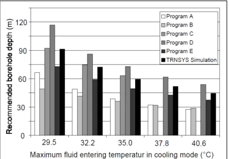
Figure 1-11 shows different simulation results comparison by Shonder et al.
Figure 1-11 Simulation programs comparison (Shonder and Hughes, 1998)
In their paper, the authors do not state the name pf the programs used, but the differences in length from the software in 1998 were disturbing. In 1999, the same authors compared a new version of the software and the results were more consistent. The lengths of boreholes varied from 7% for cooling dominated simulations to 16% for heating dominated simulations. These differences are mainly due to the assumptions made from the software (Hellström and Sanner, 2001; Shonder and al., 1999).
CHAPTER 2
SEMI-ANALYTICAL MODEL FOR GEOTHERMAL BOREFIELDS WITH INDEPENDENT INLET CONDITIONS
Patrick BELZILE, Louis LAMARCHE, Daniel R. ROUSSE
Département de génie mécanique, École de technologie supérieure, 1100, rue Notre-Dame Ouest, Montréal (Québec), Canada, H3C 1K3
Article published in “Geothermics” journal in January 2016
2.1 Abstract
A model has been developed to simulate a geothermal borefield for which borehole inlet conditions can be defined independently. The borefield is modeled with a control-volume finite difference method while boreholes are modeled as analytical thermal resistances. An analytical shape factor is used to link the borehole models to the surrounding ground models. The main advantages of the proposed model are its versatility with respect to the specification of different inlet conditions and that the temperature of the disturbed ground can be known at any point of the borefield. Application examples, coupling solar collectors and heat pumps, showed that segregating the components into two loops requires 4.3% more energy from the heat pumps than a single loop arrangement for the first five years, but will require less energy after. The examples demonstrate the interest of the proposed method.
2.2 Introduction
Geothermal heat pump systems have been in use for years in building heating, ventilation and air conditioning (HVAC) applications. District heating and cooling applications could provide an economy of scale in energy consumption for larger construction projects.
Nevertheless, when a geothermal borefield must be shared, the calculation is done in a classical manner such that each borehole in the borefield has the same inlet temperature and flow rate.
The objective of this paper is to present a geothermal model that allows independent inlet conditions for each borehole in a borefield. The interest of the method is shown by comparing the energy required from heat pumps to supply the residential heating and cooling loads in different geothermal heat pump and solar collector configurations.
In this paper, a short literature survey is presented, followed by a description of the new model for shared geothermal borefields and a comparison of different configurations of geothermal heat pump systems coupled with solar collectors.
2.3 Brief literature review
Geothermal borefield models can be organized in two categories: analytical and numerical models. The classical analytical models are: the infinite line source model (Ingersoll and Plass, 1948), infinite cylindrical source model (Ingersoll, 1954) and finite line source model (Zeng and al., 2002), including a contribution to the finite line source model (Lamarche and Beauchamp, 2007a). These models have been reviewed and their validity ranges have been compared (Philippe and al., 2009) as well as their short step-time validity (Lamarche, 2013). Most of the analytical models evaluate the mean borehole surface temperature assuming a uniform heat flow along the borehole, others evaluate the mean heat flux assuming a uniform borehole temperature (Cimmino and Bernier, 2014). In all cases, the solutions are given for a constant heat pulse, and temporal superposition is used to evaluate the effect of the variation of the heat load into the ground. Models also take thermal capacities into account to improve short time simulation results (Bauer and al., 2011; Pasquier and Marcotte, 2012).
Numerical and hybrid analytical/numerical models have been proposed: Duct Storage System (DST) (Hellström, 1991), Rottmayer’s (Rottmayer, 1997), Li’s (Li and Zheng, 2009),
Superposition Borehole method (SBM) (Eskilson and Claesson, 1988) and Koohi-Fayegh and Rosen’s (Koohi-Fayegh and Rosen, 2014).
Among these, Eskilson and Claesson use a finite difference method, with 2-D axisymmetric coordinates, to evaluate the impact of time-dependent step heat extraction or injection, and superpose them. The authors compute dimensionless temperature response factors (g-functions). The axial conductive heat transfer is incorporated in the numerical model by an analytical solution.
When more than one borehole heat exchangers are close to another, the heat transferred to the ground by each of them can influence the behaviour of the others. The boreholes are usually coupled in parallel and the temperature at which the fluid enters each borehole is the same, but different when it exists. Factors that influence this interaction are evaluated as “temperature penalty” (ASHRAE, 2007), g-functions (Eskilson, 1987) and have been studied in a 2D finite element model (Koohi-Fayegh and Rosen, 2012). These factors include the distance between the boreholes, the heat flux from the borehole wall, the time of system operation and ground properties.
Using the finite difference method and an analytical model, the DST model estimates the behavior of a geothermal borefield through time. The method is described in a manual supplied with the TRNSYS® software (TRNSYS, 2011b) (Hellström, 1989) and in Chapuis’ thesis (Chapuis, 2008). The DST model is divided into three parts: local process, global process, and steady flux. The borehole resistance (R’b) is based on the Hellström line-source
model (Hellström, 1991). The DST simulation model (Hellström, 1989; Pahud and al., 1996) can only simulate one inlet temperature and flow rate in borefields and the boreholes are considered as uniformly distributed in the borefield. All of these models are valid for a minimum period of a few hours.
Work has been done to shorten the time-step of different methods: Yavusturk (Yavuzturk and Spitler, 1999) developed a short time-step (one hour or less) model for vertical boreholes. Li
developed a 3D unstructured finite volume model using Delaunay’s triangulation mesh method (Li and Zheng, 2009). The model divides the ground into layers to take fluid temperature variation into account. It also considers the interaction between the legs of the U-tube. More recently, a study modeled the two legs of a U-tube as a single equivalent pipe in an analytical model (Claesson and Javed, 2011).
A spectral model has been developed for shallow geothermal systems (Al-Khoury, 2011). The problem is solved using the discrete Fourier transform and takes into account axial temperature variations.
Many models exist to evaluate a borehole’s thermal resistance (R’b). Some are 2D models:
Paul (Paul, 1996), Sharqawy (Sharqawy, 2008), Line-source (Hellström, 1991), and Multipole (Bennet and al., 1987). Others are quasi 3D models to take into account the axial heat transfer: Zeng (Zeng and al., 2003), P-linear (Marcotte and Pasquier, 2008) and Spectral (Al-Khoury, 2011).
These models were compared in a 2D and 3D finite element analysis using COMSOL® (Lamarche and al., 2010). Generally, the 2D models gave better results for the Multipole model, except in cases for which the temperature was constant all around the borehole, such as when steel casings are used. The 3D approach, based on borehole resistance and internal resistance, showed that the Zeng contribution provides results comparable to COMSOL® results. The COMSOL® analysis was also compared with DST model results.
Finally, a network-based model allowing the simulation of different inlet conditions in boreholes of a borefield has recently been proposed by Lazzarotto (Lazzarotto, 2014).
2.4 Description of the proposed model
The proposed model is a semi-analytical model that evaluates temperature exchange between a fluid and the ground through geothermal boreholes.
For now, the numerical part uses a 2-D control volume finite difference method (CVFDM) to solve the conduction problem in the ground. As a result, the problem is assumed to be independent of depth, Lp. A point-by-point Gauss-Seidel iterative method is used to evaluate the temperature field caused by diffusion in the surrounding ground. A tri-diagonal matrix algorithm (TDMA) method was tried, but did not yield any advantage in the computational time. On structured grids, a TDMA usually decreases the CPU time as the information from the boundaries is distributed much faster within the domain. Here, the boreholes drive the problem and information comes from within the domain. This may explain the results obtained with a TDMA.
The analytical part of the model is composed of a multipole borehole thermal resistance (Claesson and Hellström, 2011). The link between the analytical and numerical parts is done with a shape factor, under a quasi-steady-state assumption.
2.4.1 Numerical part
For a ground assumed to involve constant thermophysical properties, the two-dimensional Cartesian heat conduction governing equation in a horizontal plane is based on Fourier’s law:
s s T T T T c k S t x x y y ρ ∂∂ = ∂ ∂∂ ∂ +∂∂ ∂ ∂ + (2.1)
In eq. (2.1), the source term ST is defined by analytical models in the relevant areas of
The control volume finite difference method (CVFDM) is used to discretize the space-time domain problem in x, y, t. as most borehole arrangements have a structured pattern.
Discretization is done through a structured regular mesh. A “Type A” grid is used, which involves half-control volumes at the boundaries (Patankar, 1980). Dirichlet boundary conditions are imposed on the four boundaries considering the ground temperature is undisturbed at a certain distance from the boreholes. Standard interpolation functions for properties and dependent variables are implemented, but not used as the properties are assumed to be constant (Patankar, 1980) in this first work on the subject.
2.4.2 Analytical part
The heat rate between the borehole heat exchanger and the surrounding ground is calculated from the convective heat transfer of the fluid passing through the U-tubes of the boreholes.
(
, ,)
f f f in f out
q m c T= −T (2.2)
As the problem is considered independent of depth Lb, from eq. (2.2), the source term in eq. (2.1) can be determined such that:
T b q q S dV dx dy L = = ⋅ ⋅ (2.3)
But the outlet temperature, Tf,out must be determined to calculate this source term. And this is
the subject matter of this section.
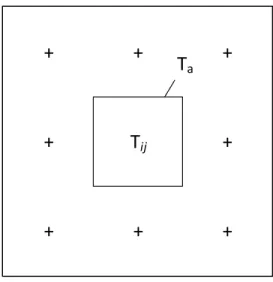
First, the ground surrounding a borehole is modeled as a square control volume for which the thermal properties are uniform and constant and for which the boundary temperature is uniform at T = Ta. The inner borehole is then assumed to be at a fixed and uniform
temperature T = Tb. Figure 2-1 depicts the relationship between the CV boundary and the
Figure 2-1 Shape factor
The heat flux equation per unit depth between the borehole (surface b) and the control-volume (surface a) is then given by:
(
) (
)
' ' b a s b a b c T T S k q T T L R − × = − = (2.4)For the above-prescribed assumptions, the shape factor S is readily given by (Incropera and DeWitt, 2007):
2 ln 1.8 b L S W D π = (2.5)
The unit length resistance Rc’ can be introduced such that:
b c s L R S k ′ = × (2.6)
which represents the resistance to the conductive heat transfer between surface a and surface b.
But still the borehole temperature, Tb, is unknown. Then, the Multipole borehole thermal model proposed by Claesson and Hellström (2011) is employed. This model evaluates thermal interaction between pipes inserted in a cylinder. The resulting borehole thermal resistances, Ra’, Rb’, R1’, R2’, R12’, are functions of geometrical parameters, such as the radii
W
Tb Ta
of the borehole and the pipes and distance between the pipes, as well as thermal properties of the pipe, grout, and the surrounding ground.
Hence, the heat flux between the fluid circulating in the pipe and the surrounding control volumes can be represented by the thermal resistance analogy, as shown in Figure 2-2.
Figure 2-2 Combined borehole and shape factor thermal
resistance analogy
The outlet fluid temperature Tf,out is a function of the average ground temperature Ta. This
temperature is evaluated from a weighted average of the nine ground control volume temperatures adjacent and contiguous for which the central control volume embeds a borehole, as depicted in Figure 2-3.
Rc Control Volume Borehole R’12 Tij Tf2 Tf1
Figure 2-3 Ground temperature surrounding a source term
Hence, Ta is defined such that:
, 16 16 2 i j n e s w ne se sw nw a T T T T T T T T T T = + + + + + + + + (2.7)
This equation represents the link between the CVFDM and the analytical model that can determine the source term in the energy conservation equation.
The outlet fluid temperature can be determined from the known inlet temperature. As the z-axial variations are neglected, an average fluid temperature, Tf, can be defined as the
arithmetic mean of the inlet and outlet temperature such that:
, , 2 f in f out f T T T = + (2.8)
Tf,out can be explicitly expressed, see eq.(2.2), such that:
, , b f out f in f f q L T T m c ′ = − (2.9)