The psml format and library for norm-conserving pseudopotential data curation and interoperability

The psml format and library for norm-conserving

pseudopotential data curation and interoperability

Alberto Garc´ıaa,∗, Matthieu Verstraeteb, Yann Pouillonc, Javier Junquerac

a _{Institut de Ci`encia de Materials de Barcelona (ICMAB-CSIC), Campus UAB, 08193}

Bellaterra, Spain

b_{nanomat/Q-MAT/CESAM, Universit´e de Li`ege, All´ee du 6 Aoˆut 19 (B5a), B-4000 Li`ege,}

Belgium

c_{Departamento de Ciencias de la Tierra y F´ısica de la Materia Condensada, Universidad}

de Cantabria, Cantabria Campus Internacional, Avenida de los Castros s/n, 39005 Santander, Spain

Abstract

Norm-conserving pseudopotentials are used by a significant number of electronic-structure packages, but the practical differences among codes in the handling of the associated data hinder their interoperability and make it difficult to com-pare their results. At the same time, existing formats lack provenance data, which makes it difficult to track and document computational workflows. To address these problems, we first propose a file format (psml) that maps the basic concepts of the norm-conserving pseudopotential domain in a flexible form and supports the inclusion of provenance information and other important metadata. Second, we provide a software library (libPSML) that can be used by electronic structure codes to transparently extract the information in the file and adapt it to their own data structures, or to create converters for other formats. Support for the new file format has been already implemented in several pseudopotential generator programs (including atom and oncvpsp), and the library has been linked with siesta and abinit, allowing them to work with the same pseudopo-tential operator (with the same local part and fully non-local projectors) thus easing the comparison of their results for the structural and electronic prop-erties, as shown for several example systems. This methodology can be easily transferred to any other package that uses norm-conserving pseudopotentials, and offers a proof-of-concept for a general approach to interoperability.

PACS: 71.15.Dx 71.10.-w

31.15.E-Keywords: Pseudopotential, Density functional, Electronic Structure

∗_{Corresponding author}

Email addresses: albertog@icmab.es (Alberto Garc´ıa),

Matthieu.Verstraete@ulg.ac.be ( Matthieu Verstraete ), yann.pouillon@unican.es ( Yann Pouillon ), javier.junquera@unican.es ( Javier Junquera )

PROGRAM SUMMARY

Program Title: libPSML

Licensing provisions: BSD 3-clause Programming language: Fortran Distribution format: tar.gz

External routines/libraries: xmlf90 for XML handling in Fortran (http://launchpad.net/xmlf90) Nature of problem:

Enhancing the interoperability of electronic-structure codes by sharing pseudopoten-tial data.

Solution method:

Create an XML-based pseudopotential format (psml), complete with a formal schema, and a processing library (libPSML) that transparently connects client codes to the in-formation in the format.

1. Introduction

Within computational science, reproducibility of research goes beyond using a specific version of a code and the appropriate input files. What is really sought is to replicate a certain physical result with a different code which implements the same basic equations of the domain at hand, but with a different set of approximations or details of implementation. This latter code will most likely have a different input data format, which might not be perfectly mapped to the format used by the original code. Reproducibility is still possible if the input data are curated so that their essential ontological properties are preserved, since it can be assumed that properly implemented codes within a domain will share a basic ontology for this domain, and can properly interpret its elements. Here we are concerned with electronic structure methods in the broad sense [1, 2], and in particular density functional theory (DFT [3, 4]), which have become standard theoretical tools to analyze and explain experiments in chemistry, spec-troscopy, solid state physics, material science, biology, and geology, among many other fields.

Programs which implement DFT fall into two main categories, those which treat all electrons explicitly (linear augmented plane wave, LAPW [5, 6], linear muffin tin orbitals, LMTO [5, 7], or the Korringa-Kohn-Rostoker and related multiple-scattering theory methods, KKR [8, 9]), and those which replace the effect of the chemically inert core electrons by a (usually non-local) pseudopotential [10, 11, 12].

After some historical initial attempts, seminal work by Hamann, Schl¨uter and Chiang [12] and Kerker [13] showed how norm-conserving pseudopotentials achieve a good tradeoff between transferability (a pseudopotential constructed for a spe-cific environment, usually the isolated atom, gives good results when the atom is placed in a different environment) and softness (as measured for example by the number of plane waves that must be used in the representation of the wave functions for a good convergence of the physical properties). Since the 1990s more sophisticated schemes have been developed to treat the basic problem of

eliding the core electrons. In particular, ultrasoft pseudopotentials [14], and the Projector Augmented Wave (PAW) method [15] are in widespread use for their improved accuracy and features, although they involve a significantly higher degree of complexity in the implementation and maintenance of the algorithms for electronic structure determination and analysis.

Several well-known atomic DFT programs [16, 17, 18, 19, 20, 21] generate pseu-dopotentials in a variety of formats, tailored to the needs of electronic-structure codes. While some generators are now able to output data in different bespoke formats, and some simulation codes are now able to read different pseudopo-tential formats, the common historical pattern in the design of those formats has been that a generator produced data for a single particular simulation code, most likely maintained by the same group. This implied that a number of im-plicit assumptions, shared by generator and user, have gone into the formats and fossilized there. Examples include, among others, many flavours of radial grids (from linear [20, 22] to logarithmic [19, 23], including all kinds of powers [24] or geometrical series [16, 25]), different ways of storing radial functions with spherical symmetry (angularly integrated with 4πr2 factors included, where r stands for the distance to the nuclei, or multiplication by different powers of r considered), different normalization conditions, etc. This leads to practical problems, not only of programming, but of interoperability and reproducibil-ity, which depend on spelling out quite a number of details which are not well represented for all codes in existing formats.

Moreover, pseudopotential information can be produced and used at various levels. The original work was based on a set of semi-local operators (non-local in the angular part and local in the radial part), whereas very soon a compu-tationally more efficient form based on fully non-local projectors plus a local part [26] was developed, and is now the standard norm-conserving form used by electronic-structure codes. The transformation of a semi-local pseudopoten-tial into a fully non-local operator is not univocally defined from the semi-local components alone. Therefore, different codes can yield different results even if reading the same semi-local information from an input file. For example, most plane waves codes make the so-called local part equal to one of the semilocal components for reasons of efficiency, whereas siesta optimizes the local part for smoothness, since it is the only pseudopotential part that needs to be rep-resented in a real space grid [27]. Modern pseudopotential generators are able to produce directly a set of non-local operators plus a local part. True inter-operability can be achieved only if the codes use the same final projector-based pseudopotential.

Straightfoward interoperability of codes would allow all to benefit from the best capabilities of each. On the one hand, removing the variability associated with the pseudopotential would enable a direct test of the quality of the basis sets used in the expansion of the one-particle Kohn-Sham eigenstates by different codes (with identical pseudopotentials, and at convergency, one should get the same total energy for the same atomic structure with any code). On the other hand, we can imagine a situation where the most stable atomic configuration of a large system can be found with a given code in a cheap yet accurate way,

and then passed to another for further analysis through single-shot expensive calculations for the fixed geometry.

The obvious benefits of interoperability have naturally spawned efforts at provid-ing more appropriate data mechanisms. At the most basic level, some pseudopo-tential generators (e.g. oncvpsp or ape) offer options to write different output files suitable for different electronic-structure codes. While this addresses some of the problems, it falls short of a fully satisfactory solution. More robust are ef-forts to provide a standard format that can be used universally. Within the PAW domain, the PAW-XML format [28] comes close to this goal, being produced by a number of PAW dataset generators and read by most PAW-enabled electronic-structure codes. The UPF (Unified Pseudopotential Format) [29] is meant to encompass the full range of pseudopotential options, including (semi)local and fully-non-local norm-conserving, ultrasoft pseudopotentials, and PAW datasets. It is used within the Quantum Espresso suite of codes and converters exist for other codes.

We believe that, indeed, the solution to the interoperability problems involves the design a data format that faithfully maps the relevant concepts of the do-main’s ontology at all the relevant levels (semi-local pseudopotentials, charge densities, non-local projectors, local potentials, etc). But the format must also provide appropriate metadata that represents provenance (generation and any further processing) and documents in a parseable form any details that might be needed downstream. This second aspect has not been properly addressed so far.

The need for standardisation of the pseudopotential format and the provision of richer metadata to track provenance and document computational workflows has been made more relevant by the appearance during the last few years of high-throughput simulation schemes for materials design [30, 31, 32], which need well-tested and efficient pseudopotential libraries to draw upon. Examples of the latter are the ultrasoft pseudopotential library by Garrity, Bennett, Rabe and Vanderbilt [33, 34], the PSLibrary associated with QE [35], the Jollet-Torrent-Holzwarth [36] PAW library, and the libraries being built [37, 38, 39] using multi-projector norm-conserving pseudopotentials generated by the oncvpsp code [22]. The latter are proving competitive with ultrasoft pseudopotentials and the PAW method in accuracy. [38, 39]

Motivated by the all the previous considerations, in this paper we present a file format for pseudopotential data (psml, for PSeudopotential Markup Language) which is designed to encapsulate as much as possible the abstract concepts in the domain’s ontology, and to provide appropriate metadata and provenance information. Moreover, we provide a software library (libPSML) that can be used by electronic structure codes to transparently extract the information in a psml file and adapt it to their own data structures, or to create converters for other formats. Our initial focus is the sub-domain in which norm-conserving pseudopotentials are used, which is not restricted to legacy cases but is set to grow in importance due to the new multi-projector pseudopotentials mentioned above. As the format is based on XML (eXtensible Markup Language) [40], it is very flexible and can serve as a basis for the future accomodation of PAW

datasets and ultrasoft pseudopotentials. Our work falls within the scope of CE-CAM’s Electronic Structure Library (ESL) initiative [41], which aims at build-ing a collection of software functionalities, includbuild-ing standards and interfaces, to facilitate the development of electronic structure codes.

This paper is organized as follows: Section 2 describes the basic elements and structure of a psml file, with a more formal XML schema given in Sec. 3. The libPSML library is described in Sec. 4. Section 5 discusses the relationship of the current work to previous efforts, and provides a guide to the tools already available in the psml ecosystem and the mechanisms available for development of new ones. Finally, as an example of the interoperability benefits afforded by psml, we present in Sec. 6 a comparison of actual physical results obtained by abinit and siesta using the same psml files.

2. The psml file format

This section contains a design rationale and human-readable description of the format. A formal schema specification can be found in Sec. 3. The fol-lowing documents version 1.1 of the psml, current as of this writing. Any updates and complementary information are available at the ESL psml site: http://esl.cecam.org/PSML.

2.1. Root element

The root element is <psml>, containing a version attribute for use by parsers, and two attributes to make explicit the (mandatory for now) units used through-out the file: energy-unit (hartree) and length-unit (bohr). In addition, the root element should contain a uuid attribute to hold a universally unique identi-fier [42].

2.2. Provenance element(s)

The file should contain metadata concerning its own origin, to aid reproducibil-ity. As a minimum, it should contain information about the program(s) used to generate or transform the pseudopotential, ideally with version numbers and compilation options, and provide a copy of any input files fed into the pro-gram(s). The information is contained in <provenance> elements (an example is provided in Table 1). Its internal structure is subject to a minimal specifica-tion:

• The attribute creator, where the name of the generator code is specified, is mandatory.

• The attribute date is mandatory.

• If input files are provided, they should be included as <input-file> ele-ments with the single attribute name and no children other than charac-ter data, which should be placed in a CDATA section to avoid processing of XML reserved characters. For obvious reasons, the name of the file

and its detailed content will depend on the program used to generate the pseudopotential. The name should be a mnemonic reference.

• The inclusion of an <annotation> element, providing arbitrary extra infor-mation in the form of key-value pairs, is encouraged. See the description and motivation of the <annotation> element in Sec. 2.10.

There can be an arbitrary number of <provenance> elements, ordered in tempo-ral sequence in the file, with the most recent first. Since some XML processors might not preserve the order of the elements, it is suggested that a record-number attribute be added to make the temporal ordering explicit, with “1” for the oldest operation, “2” for the second oldest, and so on.

This feature supports the documentation of successive actions taken on the file’s information. For example, a pseudopotential-generation program might gener-ate a psml file containing only semilocal potentials. This file is then processed by another program that generates a local potential and the corresponding non-local projectors. The psml file produced by the second program should keep the original provenance element, and add another one detailing the extra operations taken.

Table 1: An example of the <provenance> element < ? xml v e r s i o n = " 1.0 " e n c o d i n g = " UTF -8 " ? > < p s m l v e r s i o n = " 1.1 " e n e r g y _ u n i t = " h a r t r e e " l e n g t h _ u n i t = " b o h r " u u i d = " 9 0 4 2 7 2 c0 - e496 -11 e6 - 4 9 6 d -7 f 3 0 f f 5 a 9 a 4 e " x m l n s = " h t t p : // esl . c e c a m . org / P S M L / ns / 1 . 1 " > < p r o v e n a n c e c r e a t o r = " A T M 4 . 1 . 3 " d a t e = " 23 - JUN -17 " > < a n n o t a t i o n a c t i o n = " s e m i l o c a l - p o t e n t i a l - g e n e r a t i o n " > < input - f i l e n a m e = " INP " > < ! [ C D A T A [# # PS g e n e r a t i o n w i t h c o r e c o r r e c t i o n s

# GGA ( Perdew - Burke - E r n z e r h o f ) XC , r e l a t i v i s t i c # 3 d7 4 s1 c o n f i g u r a t i o n # pe Fe , GGA , r c o r e = 0 . 7 0 tm2 3.0 n = Fe c = pbr 0.0 0.0 0.0 0.0 0.0 0.0 5 4 4 0 1 . 0 0 0 . 0 0 # 4 s1 4 1 0 . 0 0 0 . 0 0 # 4 p0 3 2 7 . 0 0 0 . 0 0 # 3 d7 4 3 0 . 0 0 0 . 0 0 # 4 f0 2 . 0 0 2 . 0 0 2 . 0 0 2 . 0 0 0 . 0 0 0 . 7 0 # | # R a d i u s of p s e u d o c o r e ]] > < / input - f i l e > < / p r o v e n a n c e >

2.3. Pseudo-atom specification

The <pseudo-atom-spec> element contains basic information about the chemical element, the generation configuration, and the type of calculation.

Element identification is in principle straightforward, with either the atomic number or the chemical symbol. However, in the interest of generality, and to cover special cases, such as synthetic (alchemical) atoms, the chemical symbol can be an arbitrary label, given by the attribute atomic-label (with the con-vention that when possible the first two characters give the standard chemical symbol) and the atomic number a real number instead of a simple integer, given by the attribute atomic-number.

The atomic calculation can be done non-relativistically, with scalar-relativistic corrections (i.e., with the mass and Darwin terms) [43, 44], or with the full Dirac equation, including spin-orbit effects. In the latter case, the (semilocal) pseudopotentials are typically provided in two sets: the degeneracy-averaged j = l + 1/2 and j = l − 1/2 components, appropriate for scalar-relativistic use, and the spin-orbit components [45].

It is also possible to carry out a non-relativistic calculation for a spin-polarized reference configuration (using spin-DFT). Standard practice is then to keep only the population-averaged pseudopotentials, as a closed-shell frozen core should not be represented by a spin-dependent potential. (But see Ref. [46] for a different point of view.)

In practice, then, one might have a primary set of l-dependent Vl(r) potentials, possibly the result of averaging, and, in the case of fully-relativistic calculations, a spin-orbit set. In other cases, the generation program might output the orig-inal lj versions in the Dirac case, or the “up” and “down” components for a spin-DFT calculation.

We cover all these possibilities in psml by using the attribute relativity, with possible values “no”, “scalar” or “dirac”, and the optional attribute spin-dft to indicate (with value “yes”) a non-relativistic spin-DFT calculation. Further, as detailed below, we provide support for the possible presence of various sets of magnitudes.

The pseudopotential construction is fundamentally dependent on the core-valence split. In most cases it is clear which states are to be considered as “valence”, and which ones are to be kept in the frozen core. However, there are borderline cases in which one has the option to treat as “valence” so-called “semicore” states which are relatively shallow and/or exhibit a sizable overlap with proper valence states.

This information is provided in the mandatory <valence-configuration> element, which details the valence configuration used at the time of pseudopotential gen-eration, given by the n and l quantum numbers, and the electronic occupation of each shell. Empty shells can be omitted. In DFT calculations, the spin-up and spin-down occspin-upations are also given. This element has a mandatory attribute total-valence-charge which contains the total integrated valence charge Qval for the configuration used to generate the pseudopotential.

valence shells, but for completeness it can be given in the optional <core-configuration> element, with the same structure. This tag would be useful, for example, if a core-hole pseudopotential has been created [47].

The difference between the number of protons in the nucleus and the sum of the populations of the core shells is the effective atomic number of the pseudo-atom Zpseudo, which must be given in the mandatory attribute z-pseudo.

The “pseudization flavor” or, more properly, a succint identifier for the proce-dure for pseudopotential generation, is encoded in the optional flavor attribute. If not present, more specific values can be given per pseudopotential block and per pseudization channel (see below).

If non-linear core-corrections [48] are present, the optional core-corrections at-tribute must be set to “yes”.

One further piece of information is needed to complete the general specification of the computational framework: the type of exchange-correlation (XC) func-tional(s) used. With the explosive growth in the number of functionals, it is imperative that a robust naming convention be used. In the absence of a general registry of universally-agreed names, we propose a dual naming scheme. The element <exchange-correlation> contains:

• A mandatory element <libxc-info> that maps whatever XC functional is used in the generation code to the standard set of functionals in the Libxc library [49, 50]. This library supports a large number of functionals, and new ones are added promptly as their details are published. We thus require that pseudopotential-generation programs producing psml files, and programs using the psml format, provide internal tables mapping any built-in XC naming schemes to the Libxc one. This element has the attribute number-of-functionals, and as many <functional> elements as indicated by this attribute, with attributes name, and id, as shown in the example of Table 2. These correspond to the Libxc identification standard. The attribute type (with values “exchange”, “correlation”, or “exchange-correlation”) is optional. Further, to support arbitrary mix-tures of functionals, the optional attribute weight can also be indicated. • An (optional) element <annotation> (see Sec. 2.10) that can contain any

XC identification used by the creator of the file, in the form of attribute-value pairs. This information can be read in an ad-hoc fashion by client programs, but it is obviously not as complete or robust as that contained in the <libxc-info>. For maximum interoperability, client programs should thus implement an interface to Libxc.

An optional <annotation> element can also be included inside the <pseudo-atom-spec> element. Note that the ordering of child elements is significant (see Sec. 3).

2.4. Radial functions and grid specification

At the core of this new format we face the problem of how to store a vari-ety of different radial functions (semilocal pseudopotentials, projectors, pseudo

Table 2: An example of the <pseudo-atom-spec> element

< pseudo - atom - s p e c atomic - l a b e l = " Se " z - p s e u d o = " 6 " atomic - n u m b e r = " 34 " f l a v o r = " T r o u l l i e r - M a r t i n s " r e l a t i v i t y = " d i r a c " spin - dft = " no "

core - c o r r e c t i o n s = " yes " > < e x c h a n g e - c o r r e l a t i o n >

< a n n o t a t i o n oncvpsp - xc - c o d e = " 3 "

oncvpsp - xc - t y p e = " LDA - - C e p e r l e y - A l d e r Perdew - Z u n g e r " / > < libxc - i n f o number - of - f u n c t i o n a l s = " 2 " >

< f u n c t i o n a l n a m e = " S l a t e r e x c h a n g e ( LDA ) " t y p e = " e x c h a n g e " id = " 1 " / >

< f u n c t i o n a l n a m e = " P e r d e w & amp ; Z u n g e r ( LDA ) " t y p e = " c o r r e l a t i o n " id = " 9 " / > < / libxc - i n f o >

< / e x c h a n g e - c o r r e l a t i o n >

< valence - c o n f i g u r a t i o n total - valence - c h a r g e = " 6 " > < s h e l l n = " 4 " l = " s " o c c u p a t i o n = " 2 " / >

< s h e l l n = " 4 " l = " p " o c c u p a t i o n = " 4 " / > < / valence - c o n f i g u r a t i o n >

< / pseudo - atom - s p e c >

wave-functions, pseudocore and valence charges, etc.) in a radial grid. Most pseudopotential-generation codes export their data for their radial functions f (r) as a tabulation {f (ri)}, where {ri} are discrete values of the radial coor-dinate in an appropriate mesh.

A variety of meshes with different functional forms and parametrization details are in common use. Our preferred way to handle this variety of choices is to specify the actual grid point data in the file. This is most extensible to any kind of grid, and avoids problems of interpretation of the parameters, starting and ending points, etc. Furthermore, as explained below, the psml handling library is completely grid-agnostic, since evaluators are provided for the relevant functions f (r), in such a way that a client code can obtain the value of f at any radial coordinate r, in particular at the points of a grid of its own choosing. The precision of the computed value f (r) is of course dependent on the quality of the f (ri) tabulation in the first place, and producer codes should take this issue seriously. We discuss more points related to the evaluation of tabulated data in Sec. 4.6.

The format should be flexible enough to allow each radial function to use its own grid if needed, while providing for the most common case in which all radial functions use a common grid (or a subset of its points). Our solution is to en-code the information about each radial function in a <radfunc> element, which contains the tabulation data f (ri) in a <data> element. The grid specification uses a cascade scheme with an (optional but recommended) top-level <grid> element, optional mid-level <grid> elements under certain grouping elements, and at the lowest level optional <grid> elements inside the individual <radfunc> elements. The grid {ri} for a function is inherited from the closest <grid> ele-ment at an enclosing level if it is not specified in the local <radfunc> eleele-ment. The grouping elements currently allowed to include mid-level grids are those for semilocal potentials, nonlocal projectors, local potential, pseudo-wavefunctions, valence charge, and pseudocore charge.

The <grid> elements should have a mandatory “npts” attribute providing the number of points, and a <grid-data> element with the grid point data as for-matted real numbers with appropriate precision. All radial data must be given in bohr.

For convenience, it is allowed to include an <annotation> element as child of <grid>, with appropriate attributes, to provide additional information regard-ing the form of the grid data. The client program can process this information if needed. The <data> element may contain an optional attribute npts to in-dicate the number of values that follow. In its absence, the number of values must match the size of the grid. The npts attribute is useful in those cases in which the effective range of a radial function is significatively smaller than the extent of the grid. For example, a psml file might contain a top-level grid with a large range, appropriate for the valence charge density, of which only a subset of points are used for the projectors, which have a much smaller range.

A technical point should be kept in mind. When processing a psml file, the radial function information is typically stored internally as a table on which interpolation is performed to obtain values of the function at specific radii. In order to avoid the dangers associated with extrapolation, the radial grid must contain as first point r = 0, and any radial magnitudes (pseudopotentials, wave-functions, pseudo-core or valence charges) should be given without extra factors of r that might hamper the calculation of needed values at r = 0. In this way the processor can unambiguously determine the function values at all radial points.

When evaluating a function at a point r beyond the maximum range of the tabulated data in the psml file, a processor should return:

• -Zpseudo/r for the semi-local and local pseudopotentials, in keeping with the well-known asymptotic behavior.

• Zero for projectors, pseudo-wave-functions and valence and pseudo-core charges.

Table 3: An example of the <grid> element < g r i d n p t s = " 1 1 8 6 " > < a n n o t a t i o n t y p e = " log - a t o m " n r v a l = " 1 1 8 6 " s c a l e = " 0 . 4 4 2 6 3 4 3 1 7 2 6 2 E -04 " s t e p = " 0 . 1 2 5 0 0 0 0 0 0 0 0 0 E -01 " / > < grid - d a t a > 0 . 0 0 0 0 0 0 0 0 0 0 0 0 E +00 5 . 5 6 7 6 5 4 3 0 9 9 0 0 E -07 1 . 1 2 0 5 3 4 1 0 8 9 7 3 E -06 1 . 6 9 1 3 9 4 1 2 3 9 5 3 E -06 2 . 2 6 9 4 3 4 6 7 3 9 6 7 E -06 2 . 8 5 4 7 4 6 0 7 9 0 2 8 E -06 3 . 4 4 7 4 1 9 7 9 5 2 3 4 E -06 4 . 0 4 7 5 4 8 4 2 9 0 5 8 E -06 ... < / grid - d a t a > < / g r i d >

2.5. Semilocal components of the pseudopotentials

When available, the l-dependent (or maybe lj-dependent) semilocal components Vl(r) of the pseudopotential are classified under <semilocal-potentials> elements, with attributes:

• set: A string indicating which set (see below) the potentials belong to. If missing, the information is obtained from the records for the individual potentials.

• flavor: (optional) The pseudization flavor. If missing, its value is inher-ited from the value in the <pseudo-atom-spec> element. It can also be superseded by the records for the individual potentials.

The set attribute allows the handling of various sets of pseudopotentials. Its value is normalized as follows, depending on the type of calculation generating the pseudopotential and the way in which the code chooses to present the results:

• “non relativistic” for the non-relativistic, non-spin-DFT case.

• “scalar relativistic” if the calculation is scalar-relativistic, or if it is fully relativistic and an set of lj potentials averaged over j is provided. • “spin orbit” if a fully relativistic code provides this combination of lj

potentials.

• “lj” for a fully relativistic calculation with straight output of the lj chan-nels.

• “spin average” for the spin-DFT case when the generation code outputs a population-averaged pseudopotential.

• “up” and “down”, for a spin-DFT calculation with straight output of the spin channels.

• “spin difference” for the spin-DFT case when the generation code outputs also the difference between the “up” and “down” potentials. This and the previous case are retained for historical reasons, but are likely used rarely. Note that a given code might choose to output its semilocal-potential informa-tion in two different forms (say, as scalar-relativistic and spin-orbit combinainforma-tions plus the lj form). The format allows this, although in this particular case the information can easily be converted from the lj form to the other by client programs.

For extensibility, the format allows two more values for the set attribute, “user extension1” and “user extension2”, which can in principle be used to store custom

informa-tion while maintaining structural and operative compatibility with the format. The pseudopotentials must be given in hartree.

The <semilocal-potentials> element contains child <slps> elements, which store the information for the individual semilocal pseudopotential components. The attributes of this element are:

• n: principal quantum number of the pseudized shell. • l: angular momentum number of the pseudized shell. • j: (compulsory for “lj” sets) j quantum number • rc: rc pseudization radius for this shell (in Bohr).

• eref: (optional) reference energy (eigenvalue) of the all-electron wavefunc-tion to be pseudized (in hartree).

• flavor: (optional) To allow for different schemes for different channels, the value of this attribute, when present, takes precedence over the fla-vor attributes in the <pseudo-atom-spec> element and the <semilocal-potentials> elements.

The optional attribute eref might only be meaningful for certain potentials (for example, those that have been directly generated, and are not the product of any extra conversion, such as from lj to scalar-relativistic plus spin-orbit form). Each <slps> element contains a <radfunc> element. The order in which the <slps> elements appear is irrelevant.

The <semilocal-potentials> element can contain an optional <grid> child ap-plying to all the enclosed elements, as well as an optional <annotation> element for arbitrary extra information in key-value format.

2.6. Pseudopotential in fully non-local form.

Most modern electronic-structure codes do not actually use the pseudopotential in its semi-local form, but in a more efficient fully non-local form based on short-range projectors plus a “local” potential:

ˆ

Vps= ˆVlocal+ X

i

|χi> EKBi < χi| (1)

proposed originally by Kleinman and Bylander [26] and generalized among oth-ers by Bl¨ochl [15], Vanderbilt [14], and Hamann [22].

The information about this operator form of the pseudopotential is split in two elements, holding the local potential and the nonlocal projectors.

2.6.1. Local potential

The <local-potential> element has the attribute

• type We suggest the string “l=X” when the local potential is taken to be the semi-local component for channel “X”, or any other succint comment if not.

and contains a <radfunc> element with the actual data for the local pseudopo-tential.

Optionally, the <local-potential> element can contain a child <local-charge> element, describing a radial function ρlocal(r) related to Vlocal(r) by Poisson’s

equation. That is, ρlocal(r), integrating to Zpseudo and localized in the core re-gion, is the effective charge that would generate Vlocal(r). The <local-charge> element is optional because not all Vlocal(r) functions are representable as orig-inating from a charge distribution (V0local(0) must be zero for this). When it is present, however, it can save some client programs (such as siesta, which uses ρlocal(r) to generate a very convenient localized neutral-atom potential) the task of computing numerical derivatives of Vlocal(r).

The <local-potential> element can also contain an optional <grid> child apply-ing to all the enclosed elements, as well as an optional <annotation> element for arbitrary extra information in key-value format.

2.6.2. Non-local projectors

The information about the non-local projectors is stored in <nonlocal-projectors> elements, with the optional attribute set, as above, containing <proj> elements with attributes

• ekb: Prefactor of the projector in the corresponding term in Eq. 1 (in hartree).

• eref: (optional) Reference energy used in the generation of the projector (in hartree).

• l: angular momentum number

• j: (compulsory for “lj” sets) j quantum number

• seq: sequence number within a given l (or lj) shell, to support the case of multiple projectors.

• type: Succint comment about the kind of projector

and a <radfunc> element containing the data for the χi functions in Eq. 1. These functions are formally three-dimensional, including the appropriate

spher-ical harmonic for the angular coordinates, and a radial component: χi =

χi(r)Ylm(θ, φ). What is actually stored in the file is the function χi(r), nor-malized in the one-dimensional sense:

Z ∞ 0 r2|χi(r)| 2 dr = Z ∞ 0 |rχi(r)| 2 = 1, (2)

and proportional to rl _{near the origin.}

There can be several <nonlocal-projectors> elements, using different values for the set attribute, as explained in Sec. 2.5. For projectors in the “dirac” case, the functionality provided by the handling of set attributes can be very useful, as it is not straightforward to convert the lj information into scalar-relativistic and spin-orbit combinations. Unlike in the semi-local case, this conversion is not reversible, so the lj form is more fundamental. For maximum interoperability, producer codes should store both the lj and the combination sets.

The optional attribute eref might only be meaningful for certain projectors (for example, those that have been directly generated, and are not the product of any extra conversion, such as from lj to scalar-relativistic plus spin-orbit form).

2.7. Pseudo-wave functions

Pseudo-wavefunctions are typically produced at an intermediate stage in the generation (and testing) of a pseudopotential, but they are not strictly needed in electronic-structure codes, except in a few cases:

• When atomic-like initial wavefunctions are needed to start the electronic-structure calculation.

• When the code uses internally a fully-nonlocal form of the pseudopo-tential which is constructed from the semilocal form and the pseudo-wavefunctions.

While these pseudo-wavefunctions could be generated by the client program, we allow for the possibility of including them explicitly in the psml file. Any (optional) wavefunction data must be included in <pseudo-wave-functions> el-ements, with a set attribute and as much extra metadata as needed (which we do not try to standardize at this point, so it should be given in the form of annotations).

The extra metadata might indicate whether the data is for actual pseudized wave-functions, or for the pseudo-valence wave functions generated with the obtained pseudopotential. There might be subtle differences between them, no-tably regarding relativistic effects, as some generation codes use a non-relativistic scheme to “test” the pseudopotential and generate pseudo wavefunctions, in-stead of a scalar or fully relativistic version.

Each pswf is given in a <pswf> element, with attributes that identify the quan-tum numbers for the shell and the apropriate energy level (which could be the eigenvalue in the original pseudization, or another energy level used in the in-tegration leading to the wavefunction):

• n: principal quantum number of the shell. • l: angular momentum number of the shell. • j: (compulsory for “lj” sets) j quantum number • energy level

and a <radfunc> element.

The data is for the standard radial part of the wave function Rn,l(r), and (for bound states) should be normalized as

Z ∞ 0 r2|Rn,l(r)|2dr = Z ∞ 0 |un,l(r)|2= 1. (3)

Within our psml format R(r) is given, rather than u(r), due to the extrapolation issues detailed in the section covering the grid.

The <pseudo-wave-functions> elements can contain an optional <grid> child applying to all the enclosed elements.

2.8. Valence charge density

Some electronic-structure codes might need information about the valence charge density of the pseudo-atom. This can be the pseudo-valence charge density used to unscreen the ionic potential during the pseudopotential generation process, or the pseudo-valence charge computed from the pseudopotential itself. In psml it is given under the <valence-charge> element, whose child <radfunc> element holds a solid-angle-integrated form q(r) normalized so that:

Z ∞

0

r2q(r)dr = Q. (4)

Here Q is the total charge output, which must be stored in the total-charge attribute. The attributes is-unscreening-charge (with value “yes” or “no”) and rescaled-to-z-pseudo (“yes” or “no”) are optional.

In combination with the information in the <valence-configuration> element, these attributes will help some client codes process the valence charge density data appropriately, particularly in the case in which the pseudopotential genera-tion used an ionic configuragenera-tion. Some codes output in this case the unscreening charge rescaled to Zpseudo. The <valence-charge> can also contain an optional annotation element.

2.9. Pseudocore-charge density

An (optional) smoothed charge density matching the density of the core elec-trons beyond a certain radius, for use with a non-linear core correction scheme [48], is contained within the <pseudocore-charge> element, with the data in the same solid-angle-integrated form (and implicit units) as the valence charge, and with the extra optional attributes:

• matching-radius: The point rcoreat which the true core density is matched to the pseudo-core density.

• number-of-continuous-derivatives: In the original scheme by Louie et al. [48] the pseudo-core charge was represented by a two-parameter formula, pro-viding continuity of the first derivative only. Other typical schemes provide continuity of the second and even higher derivatives. It is expected that the number of continuous derivatives, rather than the detailed form of the matching, is of more interest to a client program.

An optional annotation element with appropriate attributes might be given to document any extra details of the model-core generation. The <pseudocore-charge> element must appear if the core-corrections attribute of the <pseudo-atom-spec> element has the value “yes”.

2.10. The handling of annotations

XML provides for built-in extensibility and client programs can use as much or as little information as needed. For the actual mapping of a domain ontology to a XML-based format, however, clients and producers have to agree on the

terms used. What has been described in the above sections is a minimal form of such a mapping, containing the basic concepts and functions needed. The extension of the format with new fixed-meaning elements and attributes would involve an updated schema and re-coding of parsers and other programs. A more light-weight solution to the extensibility issue is provided by the use of annotations, which have the morphology of XML empty elements (containing only attributes) but can appear in various places and contain arbitrary key-value pairs. Annotations provide immediate information to human readers of the psml files, and can be exploited informally by client programs to extract additional information. For the latter use, it is clear that some degree of permanence and agreed meaning should be given to annotations, but this task falls not on some central authority, but on specific codes.

Annotations are currently allowed within the following elements: <provenance>, <pseudo-atom-spec>, <exchange-correlation>, <valence-configuration>, <core-configuration>, <semilocal-potentials>, <local-potential>, <nonlocal-projectors>, <pseudo-wave-functions>, <valence-charge>, <core-charge>, and <grid>. Top-level annotations are not allowed. They properly belong in the <provenance> elements.

3. Formal specification of the psml format

We provide a formal XML schema for the psml format, given in the very read-able RELAX NG compact form [51]. This schema can be used directly for validation of psml files, or converted to an W3C schema file (using respectively the jing and trang tools of the RELAX NG project).

This is the overall structure of a psml document, showing the main building blocks. The definitions of the grammar elements are given in the next section, when the closely related API is discussed.

d e f a u l t n a m e s p a c e = " h t t p :// esl . c e c a m . org / P S M L / ns / 1 . 1 " P S M L = e l e m e n t p s m l { R o o t . A t t r i b u t e s , P r o v e n a n c e + # O n e or m o r e p r o v e n a n c e e l e m e n t s , P s e u d o A t o m S p e c , G r i d ? # O p t i o n a l top - l e v e l g r i d , V a l e n c e C h a r g e , C o r e C h a r g e ? # O p t i o n a l p s e u d o - c o r e c h a r g e , ( ( S e m i L o c a l P o t e n t i a l s + , P S O p e r a t o r ?) | ( S e m i L o c a l P o t e n t i a l s * , P S O p e r a t o r ) ) , P s e u d o W a v e F u n c t i o n s * # Z e r o or m o r e P s e u d o W a v e f u n c t i o n g r o u p s } P s e u d o A t o m S p e c = e l e m e n t pseudo - atom - s p e c { P s e u d o A t o m S p e c . A t t r i b u t e s , A n n o t a t i o n ? , E x c h a n g e C o r r e l a t i o n , V a l e n c e C o n f i g u r a t i o n , C o r e C o n f i g u r a t i o n ?

}

P S O p e r a t o r = ( L o c a l P o t e n t i a l # L o c a l p o t e n t i a l

, N o n L o c a l P r o j e c t o r s * ) # Z e r o or m o r e f u l l y n o n l o c a l g r o u p s

The quantifiers ’*’, ’+’, and ’ ?’ mean “zero or more”, “one or more”, and “at most one”, and the ’|’ sign expresses an exclusive “or” (choice) operation. Even though RELAX NG can accommodate interleaved elements, this feature is not fully representable in W3C schema, and the ordering of the elements above is strict. We use a URI in the “esl.cecam.org” domain to identify the schema namespace, but note that it is not a resolvable location.

The main feature not discussed above in Sec. 2 is the constraint of non-emptiness of the psml file: it must contain at least either a set of semilocal-potentials, or a complete pseudopotential operator consisting of a local potential and a set of nonlocal projectors. It is also possible to have a single local potential as a degenerate form of pseudopotential operator. Beyond the minimal requirements, a psml file can contain multiple occurrences of any of these elements.

4. The psml library

We provide a companion library to the psml format, libPSML, that provides transparent parsing of and data extraction from psml files, as well as basic editing and data conversion capabilities.

The library is built around a data structure of type ps t that maps the informa-tion in a psml file. Instances of this structure are populated by psml parsers, processed by intermediate utility programs, and used as handles for informa-tion retrieval by client codes through accessor routines. The library provides, in essence:

(i) A routine to parse a psml file and produce a ps object of type ps t. (ii) A routine to dump the information in a ps object to a psml file. (iii) Accessor routines to extract information from ps objects.

(iv) Some setter routines to insert specific blocks of information into ps objects. These might be used by intermediate processors or by high-level parsers. The library is written in modern Fortran and provides a high-level Fortran interface. A C/C++ interface is in preparation.

An example of use of the library is provided in Table 4.

In what follows we describe the basic exported data structures and procedures. Full documentation for the library, as well as general information about the psml format ecosystem, is available at the psml reference page under the Electronic Structure Library project website: http://esl.cecam.org/PSML.

4.1. Exported types

The library exports a few fortran derived types to represent opaque handles in the routines:

Table 4: An example of the idioms used in the libPSML library use m _ p s m l t y p e ( p s _ t ) :: ps c a l l p s m l _ r e a d e r ( f i l e n a m e , ps ) ! S e t up o u r g r i d n p t s = 4 0 0 ; d e l t a = 0 . 0 1 a l l o c a t e ( r ( n p t s )) do ir = 1 , n p t s r ( ir ) = ( ir - 1 ) * d e l t a e n d d o c a l l p s _ P o t e n t i a l _ F i l t e r ( ps , set = S E T _ S R E L , i n d e x e s = idx , n u m b e r = n p o t s ) do i = 1 , n p o t s c a l l p s _ P o t e n t i a l _ G e t ( ps , idx ( i ) , l = l , n = n , rc = rc ) ... do ir = 1 , n p t s val = p s _ P o t e n t i a l _ V a l u e ( ps , idx ( i ) , r ( ir )) ... e n d d o e n d d o • ps t

This is the type for the handle which should be passed to most routines in the API

• ps annotation t

The associated handle is used in the routines that create annotations or extract the data in them (see Section 4.9).

• ps radfunc t

This corresponds to the internal implementation of a radial function. Its use is mostly reserved for low-level operations, as the API provides con-venience evaluators for most functions.

Additionally, and to avoid ambiguities in real types, the library exports the inte-ger parameter ps real kind that represents the kind of the real numbers accepted and returned by the library.

4.2. Parsing

• psml reader (filename, ps, debug)

parses the psml file filename and populates the data structures in the handle ps. An optional debug argument determines whether the library issues debugging messages while parsing.

• ps destroy (ps)

is a low-level routine provided for completeness in cases where a pristine ps is needed for further use.

4.3. Library identification

• function ps GetLibPSMLVersion() result(version)

The version is returned as an integer with the two least significant digits associated to the patch level (for example: 1106 would correspond to the typical dot form 1.1.6).

4.4. Data accessors

The API follows closely the element structure of the psml format. Each section in the high-level document structure of Sec. 3 is mapped to a group of routines in the API. Within each, there are routines to query any internal structure (attributes, existence, number, or selection of child elements) and routines to obtain specific data items (attributes, content of child elements).

4.4.1. Root attributes

R o o t . A t t r i b u t e s = a t t r i b u t e e n e r g y _ u n i t { " h a r t r e e " } , a t t r i b u t e l e n g t h _ u n i t { " b o h r " } , a t t r i b u t e u u i d { xsd : N M T O K E N } , a t t r i b u t e v e r s i o n { xsd : d e c i m a l }

• ps RootAttributes Get (ps,uuid,version,namespace)

As in all the routines that follow, the handle ps is mandatory. All other arguments are optional, with “out” intent, and of type character(len=*). version returns the psml version of the file being processed. A given version of the library is able to process files with lower version numbers, up to a reasonable limit. For our purposes, the NMTOKEN specification refers to a string without spaces or commas.

4.4.2. Provenance data P r o v e n a n c e = e l e m e n t p r o v e n a n c e { a t t r i b u t e record - n u m b e r { xsd : p o s i t i v e I n t e g e r }? , a t t r i b u t e c r e a t o r { xsd : s t r i n g } , a t t r i b u t e d a t e { xsd : s t r i n g } , A n n o t a t i o n ? , I n p u t F i l e * # z e r o or m o r e i n p u t f i l e s } I n p u t F i l e = e l e m e n t input - f i l e { a t t r i b u t e n a m e { xsd : N M T O K E N } , # No s p a c e s or c o m m a s a l l o w e d t e x t }

As there can be several <provenance> elements, the API provides a function to enquire about their number (depth of provenance information), and a routine to get the information from a given level:

• function ps Provenance Depth(ps) result(depth) The argument depth returns an integer number.

• ps Provenance Get(ps,level,creator,date,annotation,number of input files) The integer argument level selects the provenance depth level (1 is the deepest, or older, so to get the latest record the routine should be called with level=depth as returned from the previous routine). All other ar-guments are optional with “out” intent. creator and date are strings. Here and in what follows, annotation arguments are of the opaque type ps annotation t (see Section 4.1). If there is no annotation, an empty struc-ture is returned. The information in an annotation object can be accessed using routines described in Section 4.9.

4.4.3. Pseudo-atom specification attributes and annotation

P s e u d o A t o m S p e c . A t t r i b u t e s = a t t r i b u t e atomic - l a b e l { xsd : N M T O K E N } , a t t r i b u t e atomic - n u m b e r { xsd : d o u b l e } , a t t r i b u t e z - p s e u d o { xsd : d o u b l e } , a t t r i b u t e core - c o r r e c t i o n s { " yes " | " no " } , a t t r i b u t e r e l a t i v i t y { " no " | " s c a l a r " | " d i r a c " } , a t t r i b u t e spin - dft { " yes " | " no " }? , a t t r i b u t e f l a v o r { xsd : s t r i n g }?

• ps PseudoAtomSpec Get (ps, atomic symbol, atomic label, atomic number, z pseudo, pseudo flavor, relativity, spin dft, core corrections, annotation) The arguments spin dft and core corrections are boolean, and the routine returns an empty string in flavor if the attribute is not present (recall that flavor is a cascading attribute that can be set at multiple levels). The arguments atomic number and z pseudo are reals of kind ps real kind (see Sec. 4.1). 4.4.4. Valence configuration V a l e n c e C o n f i g u r a t i o n = e l e m e n t valence - c o n f i g u r a t i o n { a t t r i b u t e total - valence - c h a r g e { xsd : d o u b l e } , A n n o t a t i o n ? , V a l e n c e S h e l l + } V a l e n c e S h e l l = S h e l l S h e l l = e l e m e n t s h e l l { a t t r i b u t e _ l , a t t r i b u t e _ n , a t t r i b u t e o c c u p a t i o n { xsd : d o u b l e } , a t t r i b u t e o c c u p a t i o n - up { xsd : d o u b l e }? , a t t r i b u t e o c c u p a t i o n - d o w n { xsd : d o u b l e }?

}

a t t r i b u t e _ l = a t t r i b u t e l { " s " | " p " | " d " | " f " | " g " }

a t t r i b u t e _ n = a t t r i b u t e n { " 1 " | " 2 " | " 3 " | " 4 " | " 5 " | " 6 " | " 7 " | " 8 " | " 9 " }

• ps ValenceConfiguration Get(ps,nshells,charge,annotation)

This routine returns (as always, in optional arguments), the values of the top-level attributes, any annotation, and the number of Shell elements, which serves as upper limit for the index i in the following routine, which extracts shell information:

• ps ValenceShell Get(ps,i,n,l,occupation,occ up,occ down)

The n and l quantum number arguments are integers (despite the use of spectroscopic symbols for the angular momentum in the format), and the occupations real.

4.4.5. Exchange and correlation

E x c h a n g e C o r r e l a t i o n = e l e m e n t e x c h a n g e - c o r r e l a t i o n { A n n o t a t i o n ? , e l e m e n t libxc - i n f o { a t t r i b u t e number - of - f u n c t i o n a l s { xsd : p o s i t i v e I n t e g e r } , L i b x c F u n c t i o n a l + } } L i b x c F u n c t i o n a l = e l e m e n t f u n c t i o n a l { a t t r i b u t e id { xsd : p o s i t i v e I n t e g e r } , a t t r i b u t e n a m e { xsd : s t r i n g } , a t t r i b u t e w e i g h t { xsd : d o u b l e }? , # a l l o w c a n o n i c a l n a m e s a n d libxc - s t y l e s y m b o l s a t t r i b u t e t y p e { " e x c h a n g e " | " c o r r e l a t i o n " | " e x c h a n g e - c o r r e l a t i o n " | " X C _ E X C H A N G E " | " X C _ C O R R E L A T I O N " | " X C _ E X C H A N G E _ C O R R E L A T I O N " }? }

The routines follow the same structure as those in the previous section. • ps ExchangeCorrelation Get(ps,annotation,n libxc functionals) • ps LibxcFunctional Get(ps,i,name,code,type,weight)

The argument type corresponds to the type of Libxc functional, and code to the id number.

4.4.6. Valence and Core Charges

V a l e n c e C h a r g e = e l e m e n t valence - c h a r g e { a t t r i b u t e total - c h a r g e { xsd : d o u b l e } , a t t r i b u t e is - u n s c r e e n i n g - c h a r g e { " yes " | " no " }? , a t t r i b u t e r e s c a l e d - to - z - p s e u d o { " yes " | " no " }? , A n n o t a t i o n ? , R a d f u n c

} # = = = = = = = = = C o r e C h a r g e = e l e m e n t p s e u d o c o r e - c h a r g e { a t t r i b u t e m a t c h i n g - r a d i u s { xsd : d o u b l e } , a t t r i b u t e number - of - c o n t i n u o u s - d e r i v a t i v e s { xsd : n o n N e g a t i v e I n t e g e r } , A n n o t a t i o n ? , R a d f u n c }

These are radial functions with some metadata in the form of attributes, an optional annotation, and a Radfunc child. The accessors have the extra optional argument func that returns a handle to a ps radfunc t object, which can later be used to get extra information.

• ps ValenceCharge Get(ps,total charge, is unscreening charge, rescaled to z pseudo, annotation,func)

The routine returns an emtpy string in is unscreening charge and rescaled to z pseudo if the attributes are not present in the psml file.

• ps CoreCharge Get(ps,rc,nderivs,annotation,func)

rc corresponds to the matching radius and nderivs to the continuity infor-mation. Negative values are returned if the corresponding attributes are not present in the file.

The func object can be used to evaluate the radial functions at a particular point r:

• function ps GetValue(func,r) result(val) but the API offers some convenience functions

• function ps ValenceCharge Value(ps,r) result(val) • function ps CoreCharge Value(ps,r) result(val) 4.4.7. Local Potential and Local Charge Density

L o c a l P o t e n t i a l = e l e m e n t local - p o t e n t i a l { a t t r i b u t e t y p e { xsd : s t r i n g } , A n n o t a t i o n ? , G r i d ? , Radfunc , L o c a l C h a r g e ? # O p t i o n a l local - c h a r g e e l e m e n t } L o c a l C h a r g e = e l e m e n t local - c h a r g e { R a d f u n c }

In this version of the API, the optional <local-charge> element is not given a first-class status. To evaluate it (if the boolean argument has local charge is true), the func local charge argument has to be used in the ps GetValue routine above. The local potential can be evaluated via the func object or with the convenience function

• function ps LocalPotential Value(ps,r) result(val) 4.4.8. Semilocal potentials S e m i L o c a l P o t e n t i a l s = e l e m e n t s e m i l o c a l - p o t e n t i a l s { a t t r i b u t e _ s e t , a t t r i b u t e f l a v o r { xsd : s t r i n g }? , A n n o t a t i o n ? , G r i d ? , P o t e n t i a l + } P o t e n t i a l = e l e m e n t s l p s { a t t r i b u t e f l a v o r { xsd : s t r i n g }? , a t t r i b u t e _ l , a t t r i b u t e _ j ? , a t t r i b u t e _ n , a t t r i b u t e rc { xsd : d o u b l e } , a t t r i b u t e e r e f { xsd : d o u b l e }? , R a d f u n c }

As explained in Sec. 2, there can be several <semilocal-potentials> elements corresponding to different sets. Internally, the data is built up in linked lists during the parsing stage and later all the data for the <slps> child elements are re-arranged into flat tables, which can be queried like a simple database. The table indexes for the potentials with specific quantum numbers, or set membership, can be obtained with the routine

• ps SemilocalPotentials Filter(ps,indexes in,l,j,n,set,indexes,number) Here, the optional argument (of intent “in”) indexes in is an integer array containing a set of indexes on which to perform the filtering operation. If not present, the full table is used. The optional arguments l,j,n,set are the values corresponding to the filtering criteria. Upon return, the optional argument indexes would contain the set of indexes which match all the specified criteria, and number the total number of matches.

The set argument has to be given using special integer symbols exported by the API: SET SREL, SET NONREL, SET SO, SET LJ, SET UP, SET DOWN, SET SPINAVE, SET SPINDIFF, or the wildcard specifier SET ALL. An ex-ample of the use of this routine has already been given in Table 4.

The appropriate indexes can then be fed into the following routines to get specific information:

All arguments except ps and i are optional. The value returned in set is an integer which can be converted to a mnemonic string through the str of set convenience function. The annotation returned corresponds to the optional <annotation> element of the parent block of the <slps> ele-ment.

The routine returns a very large positive value in eref if the corresponding attribute is not present in the file.

• function ps Potential Value(ps,i,r) result(val) 4.4.9. Nonlocal Projectors N o n L o c a l P r o j e c t o r s = e l e m e n t n o n l o c a l - p r o j e c t o r s { a t t r i b u t e _ s e t , A n n o t a t i o n ? , G r i d ? , P r o j e c t o r + } P r o j e c t o r = e l e m e n t p r o j { a t t r i b u t e ekb { xsd : d o u b l e } , a t t r i b u t e e r e f { xsd : d o u b l e }? , a t t r i b u t e _ l , a t t r i b u t e _ j ? , a t t r i b u t e seq { xsd : p o s i t i v e I n t e g e r } , a t t r i b u t e t y p e { xsd : s t r i n g } , R a d f u n c }+

The ideas are exactly the same as for the semilocal potentials. The relevant routines are:

• ps NonlocalProjectors Filter(ps,indexes in,l,j,seq,set,indexes,number) • ps Projector Get(ps,i,l,j,seq,set,ekb,eref,type,annotation,func)

The routine returns a very large positive value in eref if the corresponding attribute is not present in the file.

• function ps Projector Value(ps,i,r) result(val) 4.4.10. Pseudo Wavefunctions P s e u d o W a v e F u n c t i o n s = e l e m e n t pseudo - wave - f u n c t i o n s { a t t r i b u t e _ s e t , A n n o t a t i o n ? , G r i d ? , P s e u d o W f + } P s e u d o W f = e l e m e n t p s w f { a t t r i b u t e _ l , a t t r i b u t e _ j ? , a t t r i b u t e _ n , a t t r i b u t e e n e r g y _ l e v e l { xsd : d o u b l e } ? , R a d f u n c }

Again, the same strategy:

• ps PseudoWavefunctions Filter(ps,indexes in,l,j,set,indexes,number) • ps PseudoWf Get(ps,i,l,j,n,set,energy level,annotation,func)

The routine returns a very large positive value in energy level if the cor-responding attribute is not present in the file.

• function ps PseudoWf Value(ps,i,r) result(val) 4.5. Radial function and grid information

R a d f u n c = e l e m e n t r a d f u n c { G r i d ? , # O p t i o n a l g r i d e l e m e n t e l e m e n t d a t a { l i s t { xsd : d o u b l e + } # O n e or m o r e f l o a t i n g p o i n t n u m b e r s } } G r i d = e l e m e n t g r i d { a t t r i b u t e n p t s { xsd : p o s i t i v e I n t e g e r } , A n n o t a t i o n ? , e l e m e n t grid - d a t a { l i s t { xsd : d o u b l e + } # O n e or m o r e f l o a t i n g p o i n t n u m b e r s } }

In keeping with the psml philosophy of being grid-agnostic, the basic API tries to discourage the direct access to the data used in the tabulation of the radial functions. The values of the functions at a particular point r can be generally obtained through the ps (Name) Value interfaces, or through the ps GetValue interface using func objects of type ps radfunc t.

It is nevertheless possible to get annotation data for the grid of a particular radial function, or for the top-level grid, through the function

• function ps GridAnnotation(ps,func) result(annotation)

If a radial function handle func is given, the annotation for that radial function’s grid is returned. Otherwise, the return value is the annotation for the top-level grid.

4.6. The evaluation engine

In the current version of the library the evaluation of tabulated functions is performed by default with polynomial interpolation, using a slightly modified version of an algorithm borrowed (with permission) from the oncvpsp program by D.R. Hamann [20]. By default seventh-order interpolation, as in oncvpsp, is used. If the library is compiled with the appropriate pre-processor symbols, the interpolator and/or its order can be chosen at runtime, but we note that this should be considered a debugging feature, as the reproducibility of results would be hampered if client codes change the interpolation parameters at will. Generator codes should instead strive to produce data tabulations that will guarantee a given level of precision when interpolated with the default scheme,

using appropriate output grids on which to sample their internal data sets. For example, our own work on enabling psml output in oncvpsp (see below) includes diagnostic tools to check the interpolation accuracy.

Most codes use internally a non-uniform grid (e.g. logarithmic). We have found that a good choice of output grid is a subset of the producer’s working grid points that leaves out most of the very close points near the origin but maintains the rest. This can be achieved by imposing a minimum inter-point separation δ. This parameter δ can be smaller than the typical linear-grid step used currently by most codes, and still lead to smaller grids (in terms of number of points) that preserve the accuracy of the output.

High-order interpolation can lead to ringing effects (oscillations of the interpo-lating polynomial between points), notably near edge regions when the shape of the function changes abruptly. This is the case, for example, if the function drops to zero within the interpolation range as a result of cutting off a tail. The actual interpolated values will typically be very small, but might cause unde-sirable effects in the client code. To avoid this problem, the libPSML evaluator works internally with an effective end-of-range that is determined by analyzing the data values after parsing.

If needed for debugging purposes, the evaluator engine can be configured by the routine:

• ps SetEvaluatorOptions(quality level,debug, use effective range, custom interpolator) All arguments are optional, and apply globally to the operation of the

library. The custom interpolator argument is not allowed if the underlying Fortran compiler does not support procedure pointers. quality level (an integer) is by default and will typically be the interpolation order, but its meaning can change with the interpolator in use. The evaluator uses an effective range by default, as discussed above, but this feature can be turned off by setting use effective range to .false.. The debug argument will turn on any extra printing configured in the evaluator. By default, no extra printing is produced.

Finally, in case it is necessary to look at the raw tabular data for debugging purposes, the library also provides a low-level routine:

• ps GetRawData(func,rg,data)

It accepts a radial function handle func, and the grid points and the actual tabulated data are returned in rg and data, which must be passed as allocatable real arrays.

4.7. Editing of ps structures

The psml library has currently some limited support for editing the content of ps t objects from user programs. For example, such an editing might be done by a KB-projector generator to insert a new provenance record (and KB and local-potential data) in the ps t object, prior to dumping to a new psml file. Editing operations not yet supported directly by a given version can still be

carried out by a direct handling of the internal structure of the ps t object, which is for now also visible to client programs.

• ps RootAttributes Set(ps,version,uuid,namespace) • ps Provenance Add(ps,creator,date,annotation)

Annotations can be created by client programs using routines exported by the psml API (see Section 4.9).

• ps NonlocalProjectors Delete(ps) • ps LocalPotential Delete(ps)

Only “deletion” operations are supported as yet.

4.8. Dump of ps structures

The contents of a (possibly edited) ps t object can be dumped to a psml file using the routine

• ps DumpToPSMLFile (ps,fname,indent)

Here fname is the output file name, and indent is a logical variable that de-termines whether automatic indenting of elements is turned on (by default it is not).

In principle, there could be dumpers for other file formats, but their implemen-tation is better left to specialized programs that are clients of the library.

4.9. Annotation API

To support the annotation functionality (see Sec. 2.10), the library contains a module with a basic implementation of an association list (a data structure holding key-value pairs). The library exports the ps annotation t type, an empty annotation object EMPTY ANNOTATION, and the following routines:

• reset annotation(annotation)

Cleans the contents of the ps annotation t object annotation so that it can be reused.

• insert annotation pair(annotation,key,value,stat)

Inserts the key, value pair of character variables in the ps annotation t object annotation. Internally, annotation can grow as much as needed. • function nitems annotation(annotation) result(nitems)

Returns the number of key-value pairs in the annotation object • get annotation value(annotation,key,value,stat)

• get annotation value(annotation,i,value,stat)

This routine has two interfaces. The first gets the value associated to the key, and the second gets the value associated to the i’th entry in the annotation object.

• get annotation key(annotation,i,key,stat)

Gets the key of the i’th entry in the annotation object.

Together with the second form of get annotation value, this routine can be used to scan the complete annotation object. The first form of get annotation value is appropriate if the key(s) are known.

In all the above routines a non-zero stat signals an error condition.

5. Discussion: the psml model and ecosystem

Our vision for the role of psml in addressing the interoperability and documen-tation problems is as follows:

• Databases offer psml files (with smart searching made possible by the clear internal structure) and most codes use them directly. As they have full provenance and a uuid tag built in, calculations can properly document the pseudopotentials used. In some cases, specific legacy formats can also be produced from psml files.

• psml files are produced directly by most pseudopotential generators, ei-ther de novo or through conversion of existing formats (with extra meta-data added).

• The psml ideas and technology are extended to include PAW datasets and ultra-soft pseudopotentials.

The psml format is able to span a wide range of uses for norm-conserving pseu-dos, from semilocal-only data files, up to full-operator datasets, with flexibility (e.g.: cascading grids), robustness (e.g.: comprehensive exchange-correlation specification) and full provenance. It does so in an extensible manner, and we plan to adapt it to include PAW and USPP in the future.

To appreciate the place of psml in relation to similar work, we can list its strengths compared to the corresponding subset of Quantum Espresso’s UPF format (which however already supports PAW datasets and ultra-soft pseudopo-tentials):

• The psml format is accompanied by a complete stand-alone processing library that eases its adoption by client codes.

• Support for alternative forms of datasets in the same file (i.e., “scalar-relativistic” plus “spin-orbit” and/or “lj” form).

• API based on interpolation that can suit any client grid, without having to adapt the client code to the dataset grid.

• Full provenance specification, even when various codes are involved in dif-ferent stages of the pseudopotential generation (i.e., semilocal generation followed by KB transformation).

• A more complete specification of the exchange-correlation functional(s) used through a libxc-compatible scheme.

• A complete and parseable specification of the valence configuration used for generation, and of the reference energies used for the projectors.

The above list could serve also in a comparison of psml with the QSO XML-based norm-conserving pseudopotential format (See Ref. [38]).

As a proof of concept of the above vision, we have modified two different atomic pseudopotential generation codes to generate psml files, and interfaced libPSML to two electronic-structure programs.

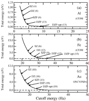
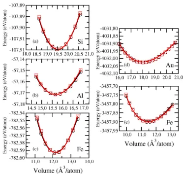
The first generator is the open-source oncvpsp code implemented by D. Hamann [22] to generate optimized multiple-projector norm-conserving pseudopotentials. The projectors are directly stored in the psml format together with the local poten-tial. In addition, a set of semi-local potentials, a by-product of the oncvpsp algorithm, is also included in the psml file. The patches needed to produce psml output in oncvpsp are available in the Launchpad code development platform [52]. To ease the production of XML, a special library (wxml, part of the xmlf90 project maintained by one of the authors (A.G.)) [53] is used. The second generator enabled for psml output is the atom code, originally developed by S. Froyen, later modified by N. Troullier and J. L. Martins, and currently maintained by one of us (A. G.) within the siesta project. atom, freely distributed to the academic community, generates norm-conserving pseu-dopotentials in the semilocal form. We have developed a post-processing tool (psop) which takes as input the semilocal components and computes a smooth local potential and the KB projector functions in the same way as it is done within the Siesta code. These new elements, together with a new provenance record, are incorporated in a new psml file, which describes a well-defined, client-code independent and unique operator.

We have thus already two different generators of psml files, their specific id-iosyncrasies being describable by a common standard. Our plans are to enable psml output in other pseudopotential-generation codes.

On the client side, we have incorporated the libPSML library in Siesta (ver-sion 4.2, soon to be released) and Abinit (ver(ver-sion 8.2 and higher). psml files can then be directly read and digested by these codes as described in Sec. 4, achieving pseudopotential interoperability between these codes, as exemplified in Sec. 6 below.

Our immediate plans include the development of a UPF-to-psml converter and to encourage the adoption of libPSML to enable the interoperability of Siesta and the codes in the Quantum Espresso suite.