Orbital and Maxillofacial Computer Aided Surgery: Patient-Specific Finite Element Models To Predict Surgical Outcomes

(1)

HAL Id: hal-00080337

https://hal.archives-ouvertes.fr/hal-00080337

Submitted on 16 Jun 2006

HAL is a multi-disciplinary open access

archive for the deposit and dissemination of sci-entific research documents, whether they are pub-lished or not. The documents may come from teaching and research institutions in France or abroad, or from public or private research centers.

L’archive ouverte pluridisciplinaire HAL, est destinée au dépôt et à la diffusion de documents scientifiques de niveau recherche, publiés ou non, émanant des établissements d’enseignement et de recherche français ou étrangers, des laboratoires publics ou privés.

Orbital and Maxillofacial Computer Aided Surgery:

Patient-Specific Finite Element Models To Predict

Surgical Outcomes

Vincent Luboz, Matthieu Chabanas, Pascal Swider, Yohan Payan

To cite this version:

Vincent Luboz, Matthieu Chabanas, Pascal Swider, Yohan Payan. Orbital and Maxillofacial Computer Aided Surgery: Patient-Specific Finite Element Models To Predict Surgical Outcomes. Computer Methods in Biomechanics and Biomedical Engineering, Taylor & Francis, 2005, 8 (4), pp.259-265. �hal-00080337�

(2)

REGULARIZATIONOFAMESHGENERATEDWITHTHE MESH-MATCHINGALGORITHM:

APPLICATION TO EXOPHTALMIA AND MAXILLOFACIAL COMPUTER AIDED SURGERY

Luboz Vincent*, Swider Pascal**, Payan Yohan*

* TIMC Laboratory, UMR CNRS 5525, University J. Fourier, 38706 La Tronche, France

** Biomechanics Laboratory, IFR 30, Purpan University Hospital, 31059 Toulouse cedex 3, France

Corresponding authors: Payan Yohan, Luboz Vincent Laboratoire TIMC/IMAG, UMR CNRS 5525,

Institut d’Ingénierie de l’Information de Santé Pavillon Taillefer – Faculté de Médecine 38706 La Tronche

France

Tel: +33 4 56 52 00 01 Fax: +33 4 56 52 00 55

(3)

ABSTRACT

Objective:

An automatic mesh regularization procedure was proposed in order to achieve the

numerical feasibility of the Finite Element Analysis.

Design:

The algorithm has been implemented for tetrahedrons, wedges and hexahedrons.

Background:

One of the main drawbacks of three-dimensional model generation is consumption due to

the manual three-dimensional meshing procedure. In a previous study, the authors

demonstrated the ability of the Mesh Matching algorithm to automatically generate

customized three-dimensional meshes from an already existing model. For anatomical

structures, some element irregularities can occur after the use of the Mesh-Matching

algorithm, making any finite element analysis impossible. Methods:

A process based on the study of the singularity of the Jacobian matrix is used to iteratively

correct them. Results:

The method was successfully evaluated on an academic test case (cubic structure meshed

with hexahedrons) and on clinical applications (face and orbit meshes).

Conclusions :

The use of the combination of the Mesh-Matching algorithm with the regularization phase

presented here seems to automatically generate new finite element meshes. Nevertheless,

no guaranty, in terms of convergence, can be given, since the regularization algorithm is

(4)

Relevance:

To our knowledge, this is the first time that an algorithm proposes to automatically

generate patient-specific finite element meshes from an existing generic finite element

mesh.

Keywords: Finite Element Modelling, Automatic Meshing, Mesh Regularization, Inference, Medical Imaging.

(5)

1. Introduction

Finite Element (FE) analysis is a widely used method in the field of biomechanics and

customized meshes are of great interest since they can integrate both geometry and

mechanical properties of the patient. Recently, the Mesh Matching (M-M) algorithm

(Couteau et al., 2000) was introduced to automatically generate customised hexahedron

and wedge 3D patient meshes from an existing 3D generic mesh. The algorithm was

successfully applied to proximal (Couteau et al, 2000) and entire (Luboz et al, 2001)

femora. However, the application to a more complicated geometry, namely a FE model of

the human face (Chabanas and Payan, 2000), provided non-satisfying mesh irregularities

that made the mechanical analysis impossible.

In commercial products, automatically meshing a 3D structure generally uses the

tetrahedral meshing technique, which is the most common form of unstructured mesh

generation. This technique is frequently based on the Delaunay criterion (Delaunay et al.,

1934) followed by the advancing front technique (Lo, 1991). The advantage of hexahedral

meshes, compared with tetrahedral meshes, is their increased accuracy. Their drawback is

that hexahedral meshing of complicated geometry is difficult (Owen, 1998) and requires a

large amount of manual intervention.

Before numerical computation can be carried out, the manually designed meshes often

need to be corrected, which is also time consuming. Several regularization techniques are

proposed in the literature and are generally adapted to tetrahedral elements. They involve a

reconnection algorithm (Joe, 1995) or a node point adjustment method (Amezua et al.,

1995). Geometrically correcting a set of elements inside a 3D mesh is a complex problem

without any straightforward solution (Cannan et al., 1993; Freitag and Plassmann, 1999).

Indeed, correcting a single element can distort its neighbours although they were originally

(6)

The goal of this study is to develop an automatic mesh regularization procedure in order

to achieve the numerical feasibility of the Finite Element Analysis. The method can be

applied to any element type (tetrahedron, hexahedron, wedge). The locations of the nodes

of irregular elements are iteratively corrected using the Jacobian determinant variations.

The method is first evaluated on an academic test case (cubic structure meshed with

hexahedrons). The method is then applied to seven human faces to investigate the

feasibility of a clinical application.

2. Materials and Methods

The patient mesh generation is obtained in two steps. First, the M-M algorithm

(Couteau et al., 2000) is applied to a standard model. Then, irregular elements that might

have been generated by the M-M algorithm are automatically regularized. This paper

focuses on the second phase and will only briefly describe the M-M algorithm.

2.1. M-M Algorithm Application The steps of the M-M algorithm:

1. A FE model of the structure is chosen. This model is often built from a standard

patient morphology. Its 3D mesh is assumed to be optimal in terms of mesh refinement

and mesh regularity. This model is called the “generic model” since it is used in the

M-M algorithm as a starting point to define other FE meshes of the same anatomical

structure corresponding to other patient morphologies.

2. The external surface of the patient anatomical structure is extracted through CT (or

MRI) acquisition. On each CT (or MRI) slice, the external contour of the structure is

(7)

3. An elastic registration method, originally proposed in the field of computer-assisted

surgery (Lavallée et al., 1995; 1996), is used to match the extracted patient surface

points with the nodes located on the external surface of the generic FE model. This

matching aims at finding a volumetric transform T, which is a combination of global

(rigid) and local (elastic) transforms. The idea underlying the matching algorithm

consists (1) in aligning the two datasets (the rigid part of T) and (2) in finding local

cubic B-Splines functions (Szeliski and Lavallée, 1996). The unknowns of the

transform are all the B-Splines parameters. Those parameters are obtained through an

optimization process (the Levenberg-Marquardt algorithm and a modified conjugate

gradient algorithm) that aims at minimizing the distance between the two surfaces,

namely the points extracted from the patient data and the external nodes of the generic

FE model.

4. The volumetric transform T is then applied to every node of the FE generic mesh,

namely the nodes located on the external surface as well as the internal nodes that

define the FE volume. A new volumetric mesh is thus automatically obtained by

assembling the transformed nodes into elements, with a topology similar to that of the

generic FE model: same number of elements and same element types.

2.2. Regularization of the Mesh 2.2.1 Regularity Criteria

Before improving the quality of the Finite Element mesh, the regularization

phase checks whether each element of the mesh is regular. This regularity notion is

associated with the Jacobian matrix transform, coupling the reference element (unit

reference framework) and the actual element (real reference framework) (Touzot and

(8)

Finite Element Analysis is carried out only if the transform can be computed on each

point inside the element, that is to say if the Jacobian determinant value (detJ) is larger

than zero anywhere inside the element. The Jacobian determinant detJ is computed at

each node of each element. If a negative or nil value is obtained for one of the nodes, the

element is classified as irregular.

2.2.2 Regularization Algorithm

The regularization algorithm consists of an iterative process: nodes of irregular

elements are slightly shifted at each step, until each element becomes regular. In the

following development, the subscript variables are: k - irregular element; i - node(s) of

element k with nil or negative Jacobian determinant; j nodes attached to element k; n

-number of nodes of element k.

The regularization procedure consists of two main steps:

- Computation of the Jacobian determinant (which has no dimension) at each node of the mesh and detection of irregular element k (detJi 0).

- Automatic correction of irregular element k using a numerical sensitivity procedure based on gradient evaluation.

The idea is to iteratively move each node i (where detJi  0) in a direction that tends to

increase the detJi value. As an analytical expression of the gradient vector (detJi)j can be

found. The algorithm consists of moving the node in the direction of the gradient vector in

order to increase detJi.

As expressed in equation (1), the gradient vector (detJi)j (whose dimension is : length

-1_{) is first computed using actual coordinates X}

(9)

element k (with a first order Taylor Series). This gradient vector provides an evaluation of

the sensitivity of the geometrical transform (reference framework / actual framework) to

the nodes locations. Analytical expressions of detJi and (detJi)j are derived using a

computer algebra system (Maple©).





                    ) ( det ) ( det ) ( det det j i j i j i j z z y y x x i i i i J J J J where j = 1...n. (1)

The directional vector Vj, expressed by equation (2), is determined for updating the

node locations. The dimension of Vj and its Euclidian norm ||Vj|| is length. For a node with

index j, the gradient vectors (1) are summed at the element k level. If n is the number of

nodes of this element k, the gradient vector is computed and summed for each node i (from

1 to n) of the element. Taking into account that only gradient vectors of irregular nodes are

summed, a coefficient i is introduced. The value of this coefficient is 1 when the

determinant of the Jacobian is negative or null at the point i and 0 when detJi is positive.

The procedure is then repeated for each distorted element and finally, the residual vector is

derived from the summation over p, p being the index of all the elements in the mesh

having the node j in their connectivity.







   n i j i p j 1 det . Ji  V ₍₂₎

where i = 1 if detJi  0 and i = 0 if detJi > 0.

The modification of node locations is based on equation (3) where Xj and X’j are the old

and the new coordinates of the node j, and w is a factor depending on the scale of the

(10)

account the dimension of the mesh. The directional vector is finally normalized with the

Euclidian norm so that Vj / ||Vj|| has no dimension.

averLength w Vj j j j X V * * X'   (3)

In addition to the algorithm, maximal node displacements are constrained so that the

regularized mesh still fits the patient morphology. The constraints for internal and external

nodes differ but they are both based on a percentage of the displacement of the nodes from

their initial positions, computed after the M-M algorithm (with a small percentage for

external surface nodes in order to still fit the patient geometry).

3. Results

The regularization method is first evaluated on the simple test case presented in Figure 1-a. The cubic structure is meshed with hexahedrons starting from a controlled irregular mesh, shown in Figure 1-b. To get this distorted mesh, the node located inside the original cube was manually moved. The minimum Jacobian determinant is - 0.1125, thus no FE analysis is feasible. The regularization method succeeded, providing a regular

mesh (figure 1-c) with a threshold value of 10-4_{for the Jacobian determinant. Increasing}

the lower admissible value of the Jacobian determinant in the algorithm also improves the meshing and allows the convergence towards perfect cubic elements (figure 1-d).

The following clinical application concerns the automatic mesh generation of human

faces in orthognatic surgery (Chabanas et al., 2003). The generic model used to run the

M-M algorithm is plotted in Figure 2a and the regularized meshing of the new patient is plotted in Figure 2b. The human face mesh is made of 2884 elements and 4216 nodes and represents the soft tissues (skin, muscles and fat tissues) as a homogenous material. The

(11)

M-M algorithm generates 149 irregular elements that were detected by the procedure. As an example, a distorted element selected within the lips is plotted before and after regularization, in Figure 2c.

It took about one minute and 130 iterations (on a DEC Alpha 500 MHz computer) to correct the irregular elements. The new mesh remains very close to the one generated by the M-M algorithm and no geometrical difference can be visually observed. More quantitatively, among the 4216 nodes of the mesh, 614 were finally moved by the iterative regularization technique, with a 2.2 mm mean displacement value (maximum displacement = 2.692 mm; minimum displacement = 0.001 mm). In this test, the Jacobian

determinant threshold value was 10-9_.

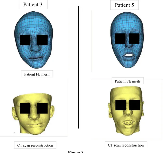
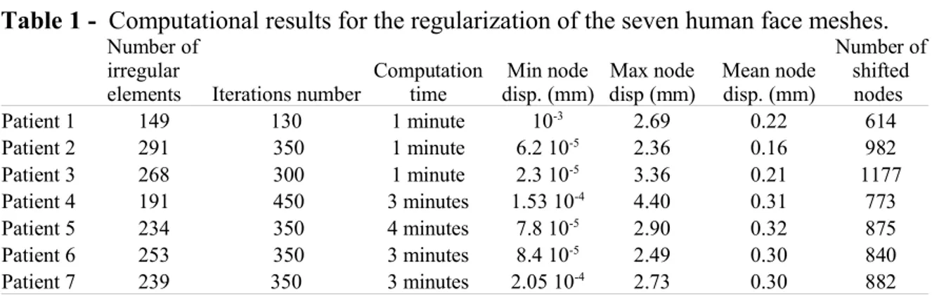
The regularization method was successfully applied to six other patient FE models generated by the M-M algorithm. Two of the six regularized meshes are presented in Figure 3. Note that the mesh after regularization is still close to the CT data. Table 1 summarizes the regularization computation time, the number of irregular nodes, node displacements and the number of shifted nodes. For all the test cases, 5% to 10% of

irregular elements have been detected and automatically regularized. Despite the obvious

variation in geometries, good results were obtained and the computation time was less

than four minutes.

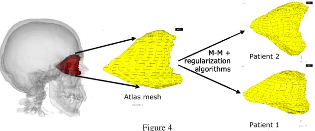
Recently, the combination of the M-M algorithm and of the regularization phase has

been applied to FE orbit meshes. As for the face, these two processes were required to

generate a great number of meshes from a manually meshed orbit used as an atlas. This

generic mesh is composed of 1375 elements and 6948 nodes and represents the soft tissues

of the orbit, i.e. the fat tissues, the muscles and the optic nerve as a homogeneous

poroelastic material. It has been developed to simulate orbital surgeries and more specially

(12)

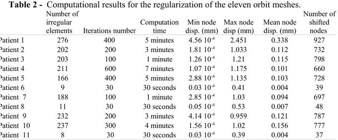
Eleven patient-specific meshes were generated with the M-M algorithm. Each mesh had

irregular elements: approximately 158 elements (with a standard deviation of 28). The

regularization phase achieved to correct all of them by moving around 566 nodes (standard

deviation: 99) with a mean displacement of 0.11 mm (standard deviation: 0.03). In this

test, the Jacobian determinant was set to 10-1_{. Table 2 summarizes the regularization}

computation time, the number of irregular nodes, node displacements and the number of shifted nodes. All irregular elements were automatically regularized by our algorithm.

Figure 4 plots two patient specific meshes thus generated and regularized. After a mean

regularization time of about 3 min (standard deviation: 40 seconds), each mesh was

corrected without any visible change in the geometry of the mesh surface.

4. Discussion and conclusion

In previous studies, it was demonstrated, for simple anatomical structures like the

femora, that the M-M algorithm is efficient at automatically generating different patient

meshes from an existing regular FE mesh. But some problems occurred when the

geometry of the modelled anatomical structure became complex. In that case, the meshes

automatically generated by the M-M algorithm were found irregular for a FE analysis. This

paper introduced a new, fully automatic regularization procedure (based on the Jacobian

determinant) that applies to these kind of irregular meshes. The procedure was illustrated

in a simple test case (cubic mesh) and it was successfully evaluated for the regularization

of seven FE meshes of the human face and eleven FE meshes of the orbit.

The regularization algorithm succeeds to automatically correct the irregular meshes

generated by the M-M method. The patient meshes can then be used to carry out a Finite

Element Analysis (in orthognatic surgery for the face model and in orbitopathy surgery for

(13)

Nevertheless, one must first notice that this regularization algorithm has been tested on

a mesh that was originally manually designed. This means that the original elements of the

generic mesh, matched to patient data with the M-M algorithm, were designed to be as

regular as possible (with hexahedrons and wedges). In other words, the generated patient

mesh was probably “less irregular” than a rough and unstructured tetrahedral mesh

deformed by the M-M algorithm would have been.

Another limitation of the method is our inability to guarantee that the regularization

algorithm will correct any irregular mesh. Indeed, due to its formulation, the iterative

process of the algorithm tries to find a global solution, without any theoretical guarantee to

converge. As can be seen on tables 1 and 2, some mesh regularizations need more

iterations than other ones, but all of them finally converge to a stable solution.

In the next phase, we plan to deal with other clinical applications involving other

geometrical FE models such as shoulder and liver. Another important perspective is to

include quality criteria for the FE mesh into the iterative regularization algorithm (warping

factor, parallel deviation, aspect ratio, edge angle, skew angle or twist angle).

Acknowledgments

Stéphane Lavallée is acknowledged for his contribution on the elastic registration

(14)

References

ANSYS, 2001, Theory Reference manual, Release 5.7.

Amezua E., Hormaza M., Hernandez A., Ajuria M.B.G., 1995. A method of the improvement of 3D solid finite-element meshes. Advances in Engineering Software, 22:45-53.

Cannan, S., Stephenson, M., Blacker, T., 1993. Optismoothing: an optimization-driven

approach to mesh smoothing. Finite Elements in Analysis and Design, 13, pp.

185-190.

Chabanas M. & Payan Y., 2000. A 3D Finite Element model of the face for simulation in plastic and maxillo-facial surgery. Proceedings of the Third International Conference on Medical Image Computing and Computer-Assisted Interventions - MICCAI'2000, October 2000, Pittsburgh, US. Springer – Verlag LNS 1935:1068-1075.

Chabanas M, Luboz V., Payan Y., 2003. Patient specific finite element model of the face for computer assisted maxillofacial surgery. Medical Image Analysis (Media).

Couteau B., Payan Y., Lavallée S., 2000. The mesh matching algorithm: an automatic 3D mesh generator for finite element structures. J. Biomechanics. 33(8): 1005-1009.

Delaunay B., 1934. Sur la sphère. Izvestia Akademia Nauk SSSR, VII Seria, Otdelenie Matematicheskii i Estestvennyka Nauk. 7:793-800.

Freitag, L.A., Plassmann, P., 1999. Local optimization-based simplicial mesh untangling

and improvement. ANL/MCS, 39, pp. 749-756.

Joe B., 1995. Construction of three-dimensional improved quality triangulations using local transformations. SIAM Journal on Scientific Computing, 16:1292-1307.

Lavallée S., Sautot P., Troccaz J., Cinquin P., Merloz P., 1995. Computer Assisted Spine

Surgery: a technique for accurate transpedicular screw fixation using CT data and a 3D

(15)

Lavallée S., 1996. Registration for Computer-Integrated Surgery: Methodology, State of the Art. In R. Taylor, S. Lavallée, G. Burdea & R. Mosges (Eds.), Computer Integrated Surgery, Cambridge, MA: MIT Press: 77-97.

Lo S. H., 1991. Volume Discretization into tetrahedra – II. 3D triangulation by advancing front approach. Computers and structures, 39(5):501-511.

Luboz V., Couteau B., Payan Y., 2001. 3D Finite element meshing of entire femora by

using the mesh matching algorithm. In Proceedings of the Transactions of the 47th

Annual Meeting of the Orthopaedic Research Society, p. 522. Transactions Editor, B. Stephen Trippel, Chicago, Illinois, USA.

LubozV., PedronoA., AmbardD., BoutaultF., PayanY., SwiderP., 2004. Prediction of

tissue decompression in orbital surgery. Clinical Biomechanics, 19(2): 202-208.

Owen S., 1998. A survey of unstructured mesh generation technology. Proceedings of the

7th_{International Meshing Roundtable, Sandia National Lab:239-267.}

Robinson J., Haggenmacher G.W., 1982. Element Warning Diagnostics. Finite Element News, June and August, 1982.

Szeliski R. and Lavallée S., 1996. Matching 3-D anatomical surfaces with non-rigid deformations using octree-splines. Int. J. of Computer Vision, 18(2): 171-186.

Touzot G., Dahtt G., 1984. Une représentation de la méthode des éléments finis. Collection université de Compiègne.

Zienkiewicz O.C., Taylor R.L., 1994. The Finite Element Method, fourth edition. McGraw-Hill Book Company.

(16)

List of figures

Figure 1 - Test case: cubic meshing. (a) perfect cubic mesh, (b) irregular mesh, (c) first

regular mesh and (d) regular mesh with detJ > 0.1.

Figure 2 – (a) generic FE mesh of the face which leads to (b) a FE mesh of a patient face

by applying the M-M algorithm. (c) example of the regularization procedure on a element.

Figure 3 - Application of the M-M algorithm and the regularization phase to two patients

with relatively different morphologies for the face. There is few visible difference between

the real morphologies (top) reconstructed using the CT scan and the FE models obtained

via the M-M algorithm coupled with the regularisation procedure.

Figure 4 - Application of the M-M algorithm and the regularization phase to two patients

with significant differences in orbit morphologies. The mesh at the left is the atlas that is

deformed to fit the morphology of the other patients, thus creating patient-specific FE

meshes.

Table 1 - Computational results for the regularization of the seven human face meshes.

(17)

REGULARIZATIONOFAMESHGENERATEDWITHTHE MESH-MATCHINGALGORITHM

Vincent Luboz,Pascal Swider, Yohan Payan

Figure 1

(a)

Perfect cubic mesh

(b)

Moved node, detJ=-0.1125

(c)

Moved node, detJ=10

-4

(d)

Moved node, detJ=10

-1

(18)

(a) (b)

(c) Figure 2

Regularized patient mesh

Generic model

Element after

regularization

Element before

regularization

(19)

Figure 3 CT scan reconstruction Patient FE mesh

Patient 5

Patient 3

CT scan reconstruction Patient FE mesh

(20)

Figure 4 Atlas mesh Patient 2 Patient 1 M-M + regularization algorithms Atlas mesh Patient 2 Patient 1 M-M + regularization algorithms Atlas mesh Patient 2 Patient 1 M-M + regularization algorithms Atlas mesh Patient 2 Patient 1 M-M + regularization algorithms

(21)

Table 1 - Computational results for the regularization of the seven human face meshes.

Number of irregular

elements Iterations number

Computation time Min node disp. (mm) Max node disp (mm) Mean node disp. (mm) Number of shifted nodes Patient 1 149 130 1 minute 10-3 2.69 0.22 614 Patient 2 291 350 1 minute 6.2 10-5 2.36 0.16 982 Patient 3 268 300 1 minute 2.3 10-5 3.36 0.21 1177 Patient 4 191 450 3 minutes 1.53 10-4 _4.40 _0.31 ₇₇₃ Patient 5 234 350 4 minutes 7.8 10-5 _2.90 _0.32 ₈₇₅ Patient 6 253 350 3 minutes 8.4 10-5 _2.49 _0.30 ₈₄₀ Patient 7 239 350 3 minutes 2.05 10-4 _2.73 _0.30 ₈₈₂

(22)

Table 2 - Computational results for the regularization of the eleven orbit meshes.

Number of irregular

elements Iterations number

Computation time Min node disp. (mm) Max node disp (mm) Mean node disp. (mm) Number of shifted nodes Patient 1 276 400 5 minutes 4.56 10-4 2.451 0.338 927 Patient 2 202 200 3 minutes 1.81 10-4 1.033 0.112 732 Patient 3 203 100 1 minute 1.26 10-4 1.21 0.115 798 Patient 4 211 600 7 minutes 1.07 10-4 _1.175 _0.101 ₆₆₀ Patient 5 166 400 5 minutes 2.88 10-4 _1.135 _0.103 ₇₂₈ Patient 6 9 30 30 seconds 0.03 10-4 _0.41 _0.004 ₃₉ Patient 7 188 100 1 minute 2.85 10-4 _1.03 _0.094 ₆₉₇ Patient 8 11 30 30 seconds 0.05 10-4 _0.53 _0.007 ₄₈ Patient 9 232 200 3 minutes 4.14 10-4 0.959 0.121 787 Patient 10 237 300 4 minutes 1.56 10-4 1.02 0.156 777 Patient 11 8 30 30 seconds 0.03 10-4 0.39 0.004 37