HAL Id: hal-00153219
https://hal.archives-ouvertes.fr/hal-00153219
Submitted on 26 Dec 2015
HAL is a multi-disciplinary open access
archive for the deposit and dissemination of
sci-entific research documents, whether they are
pub-lished or not. The documents may come from
teaching and research institutions in France or
abroad, or from public or private research centers.
L’archive ouverte pluridisciplinaire HAL, est
destinée au dépôt et à la diffusion de documents
scientifiques de niveau recherche, publiés ou non,
émanant des établissements d’enseignement et de
recherche français ou étrangers, des laboratoires
publics ou privés.
near the proton gyrofrequency in high-altitude cusp.
D. Sundkvist, A. Vaivads, M. André, J.-E. Wahlund, Y. Hobara, S. Joko, V.V.
Krasnoselskikh, Y.V. Bogdanova, S.C. Buchert, N. Cornilleau-Wehrlin, et al.
To cite this version:
D. Sundkvist, A. Vaivads, M. André, J.-E. Wahlund, Y. Hobara, et al.. Multi-spacecraft determination
of waves characteristics near the proton gyrofrequency in high-altitude cusp.. Annales Geophysicae,
European Geosciences Union, 2005, 23 (3), pp.983-995. �10.5194/angeo-23-983-2005�. �hal-00153219�
SRef-ID: 1432-0576/ag/2005-23-983 © European Geosciences Union 2005
Annales
Geophysicae
Multi-spacecraft determination of wave characteristics near the
proton gyrofrequency in high-altitude cusp
D. Sundkvist1,2,3, A. Vaivads1, M. Andr´e1, J.-E. Wahlund1, Y. Hobara4, S. Joko4, V. V. Krasnoselskikh3,
Y. V. Bogdanova5, S. C. Buchert1, N. Cornilleau-Wehrlin6, A. Fazakerley5, J.-O. Hall2, H. R`eme7, and G. Stenberg8
1Swedish Institute of Space Physics, Uppsala, Sweden
2Department of Astronomy and Space Physics, University of Uppsala, Uppsala, Sweden
3Laboratoire de Physique et Chimie de l’Environnement, CNRS, Orl´eans, France
4Swedish Institute of Space Physics, Kiruna, Sweden
5Mullard Space Science Laboratory, University College, London, UK
6Centre d’Etude des Environnements Terrestre et Planetaires, CNRS, V´elizy, France
7Centre d’Etude Spatiale des Rayonnements, CNRS, Toulouse, France
8Department of Physics, University of Ume˚a, Ume˚a, Sweden
Received: 30 September 2004 – Revised: 28 January 2005 – Accepted: 2 February 2005 – Published: 30 March 2005
Abstract. We present a detailed study of waves with fre-quencies near the proton gyrofrequency in the high-altitude cusp for northward IMF as observed by the Cluster space-craft. Waves in this regime can be important for energiza-tion of ions and electrons and for energy transfer between different plasma populations. These waves are present in the entire cusp with the highest amplitudes being associ-ated with localized regions of downward precipitating ions, most probably originating from the reconnection site at the magnetopause. The Poynting flux carried by these waves is downward/upward at frequencies below/above the proton gy-rofrequency, which is consistent with the waves being gen-erated near the local proton gyrofrequency in an extended region along the flux tube. We suggest that the waves can be generated by the precipitating ions that show shell-like distributions. There is no clear polarization of the perpen-dicular wave components with respect to the background magnetic field, while the waves are polarized in a parallel-perpendicular plane. The coherence length is of the order of one ion-gyroradius in the direction perpendicular to the am-bient magnetic field and a few times larger or more in the par-allel direction. The perpendicular phase velocity was found to be of the order of 100 km/s, an order of magnitude lower than the local Alfv´en speed. The perpendicular wavelength is of the order of a few proton gyroradius or less. Based on our multi-spacecraft observations we conclude that the waves cannot be ion-whistlers, while we suggest that the waves can belong to the kinetic Alfv´en branch below the proton
gyrofre-quency fcp and be described as non-potential ion-cyclotron
waves (electromagnetic ion-Bernstein waves) above. Linear
Correspondence to: D. Sundkvist
wave growth calculations using kinetic code show consid-erable wave growth of non-potential ion cyclotron waves at wavelengths agreeing with observations. Inhomogeneities in the plasma on the order of the ion-gyroradius suggests that inhomogeneous (drift) or nonlinear effects or both of these should be taken into account.
Keywords. Magnetospheric physics (magnetopause, cusp and boundary layers; plasma waves and instabilities) – Space plasma physics (waves and instabilities)
1 Introduction
The cusp regions of the terrestrial magnetosphere play an im-portant role in the transfer of energy from the solar wind to the ionosphere, since the cusp magnetic field lines directly connect the solar wind with the Earth’s polar regions. The cusps are also regions where efficient energization of the ionospheric plasma is taking place and energy is continu-ously transferred among different plasma populations. Most of these processes are due to different plasma waves.
Intense waves with frequencies of the order of the ion gy-rofrequency have often been observed in the cusp by several spacecraft at varying altitudes. Such waves are known to be important for energy redistribution between different parti-cle populations, e.g. via ion-cyclotron resonance. Identifi-cation of the wave generation mechanisms and wave modes are essential for the understanding of the overall cusp energy conversion processes and particle transport.
The cusp is a very structured region. Until recently
only single satellite observations have been available, with the inherent problem of distinguishing between spatial and
temporal variations. Here we analyze wave observations
ob-tained at around 8 Earth radii (RE) near noon by the four
Cluster spacecraft. We find that multi-spacecraft measure-ments are essential for understanding wave properties in the cusp.
Waves with obvious peaks in the power spectrum near the proton gyrofrequency have been observed in the auroral and cusp regions, see reviews by Gurnett (1991) and Andr´e (1997). They have been identified either as Electrostatic Ion Cyclotron (EIC) waves, typically with a spectral peak above the proton gyrofrequency (e.g. Kaufmann and Kintner, 1982; Andr´e et al., 1987; Stenberg et al., 2002), or as Electromag-netic Ion Cyclotron (EMIC) waves, usually with a peak be-low the proton gyrofrequency but sometimes also above (e.g. Temerin and Lysak, 1984; Gustafsson et al., 1990; Erland-son and Zanetti, 1998; Chaston et al., 1998, 2002; Santol´ık et al., 2002). Possible generation mechanisms include par-ticle beams along the geomagnetic field. There are several reports of EMIC specifically in the cusp (Russel et al., 1971; Scarf et al., 1972; Fredricks and Russell, 1973).
Other commonly observed types of waves have broad-band spectra, covering frequencies from below one up to at least several hundred Hz. These spectra often have no clear signature near the ion gyrofrequency (e.g. Gurnett and Frank, 1977; Kintner et al., 2000; Wahlund et al., 2003) and are of-ten associated with local ion energization (e.g. Andr´e et al., 1998; Hamrin et al., 2002; Bouhram et al., 2003a, 2003b). Several studies with Interball-1 (see Savin et al., 2004, and references therein) focus on the boundary between cusp and magnetosheath. In a region identified as the turbulent bound-ary layer in the distant cusp broadband turbulent like spec-tra are often observed. The generation mechanism of these waves and their dispersive properties are still not clear.
Recent studies using the Polar (Le et al., 2001) and Cluster (Nykyri et al., 2003, 2004) spacecraft study waves in the cusp having clear spectral peaks at frequencies near the proton gy-rofrequency. These waves were present in the cusp itself, as well as in its equator- and poleward boundaries. The average Poynting flux was found by Le et al. to be mainly earthward and the ratio of the wave electric and magnetic field ampli-tudes was close to the local Alfv´en speed. Both Nykyri et al. and Le et al. found that the waves could have both left- and right-handed polarization and different angles with respect to the ambient magnetic field. In addition, a time-domain cross correlation analysis done by Nykyri et al. showed that there is no correlation of the signals between spacecraft with separation distances as small as ∼100 km. The free energy source and generation mechanism of the waves is not clear, even though Nykyri et al. speculates that it can be due to velocity shear present in the cusp.
In our study we analyze waves in the frequency range around the proton gyrofrequency as observed in the
high-altitude cusp by the Cluster spacecraft. We particularly
concentrate on the poleward boundary of the cusp that for northward Interplanetary Magnetic Field (IMF) conditions corresponds to the region of freshly reconnected (opened) field lines. The goal of our investigation is to describe the
polarization and dispersive properties of the waves in enough detail to understand their nature (wave mode identification) and to identify the free energy source that could generate the waves.
This paper uses data from the multi-spacecraft Cluster en-counter of the high-altitude cusp on 9 March 2002. We start the observations section (2) with a general overview of the cusp crossing from a particle- and wave point of view. We then discuss measurements of the Poynting- and ion power flux and carry out a polarization analysis. Then we move on to multi-spacecraft measurements and present the results from a multi-spacecraft cross-spectral analysis. Finally, we end the observations part by showing ion distribution func-tions. The discussion of the measurements in Sect. 3 is fo-cused on wave properties, wave identification and possible wave generation mechanisms.
2 Observations
2.1 Event overview
On 9 March 2002 the Cluster spacecraft crossed the
high-altitude cusp of the Northern Hemisphere. The Cluster
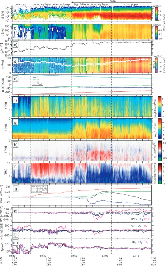
spacecraft were at the short separation of ∼100 km. All ob-servations in this section are presented for spacecraft number four (C4), although the other spacecraft observe the same characteristic features. Figure 1 shows an overview of the crossing. The Cluster spacecraft exit the polar cap and en-ter the boundary layer between the polar cap and the cusp at (1.6, –1.2, 7.6) GSM around 02:36 UT, enter the high lati-tude boundary layer (HLBL) at ∼02:49 UT, and finally enter the cusp proper at 03:02 UT (borders are marked by dotted lines in Fig. 1).
The regions are easiest to identify from Figs. 1a, b, c that show proton number flux, proton pitch angle distribution and proton density (CIS experiment, R`eme et al., 1997). The boundary layer between polar cap and cusp is characterized by the apperance of solar wind particles while their density is still very low. The cusp, consisting of both HLBL and the proper cusp, can be clearly identified as a region of high
plasma density, n>1 cm−3. The HLBL can be distinguished
by the presence of intense ion injections. In the cusp proper both up- and downgoing ions are observed, as seen from the pitch angle distribution in Fig. 1, panel (b).
The interplanetary magnetic field (ACE data time lagged by 60 min), corresponding to the Cluster cusp crossing at 02:49 UT, was (−3, 4, 2) nT (GSM). For these IMF con-ditions the expected reconnection site at the magnetopause is on the duskside, tailward from the cusp. This is consistent with the precipitating energetic ions observed by Cluster be-tween 02:49–03:02 UT being reconnection jets generated at newly-reconnected field lines. For southward IMF and low latitudes this type of plasma would be denoted as cleft or as the low-latitude boundary layer (LLBL); here observed for northward IMF we refer to it as a high-latitude boundary layer (HLBL).
Figure 1, panel (d) shows a pitch angle distribution of the electron flux centered around 130 eV (the PEACE in-strument, Johnstone et al., 1997). This energy corresponds approximately to the energy at which cusp electrons have a maximum flux and all essential electron features can be iden-tified in this panel. A significant increase in electron flux is observed at the same time as the increased proton flux around 02:49 UT. Also, one can see that there is a lower flux of electrons in the HLBL than in the proper cusp. In both re-gions the pitch-angle distribution show that the electrons are anisotropic, with the highest fluxes being along the ambient magnetic field.
The ambient magnetic field (FGM experiment, Balogh et al., 1997) during this event was of the order of 105–110 nT, and is displayed in panel (e). A continuous decrease of the magnetic field amplitude is due to the spacecraft motion to lower magnetic latitude and higher altitude. No clear de-crease in the magnetic field magnitude is associated with the cusp entrance, as is sometimes observed in the high-altitude or exterior cusp.
The above identified different regions (polar cap, bound-ary layer between polar cap and cusp, HLBL, proper cusp) also show up clearly in the plasma wave emissions. En-hanced broad-band electric field emissions, (EFW experi-ment, Gustafsson et al., 1997) are observed in the bound-ary layer between the polar cap and cusp, as well as in the HLBL but diminishes before entering the proper cusp, shown in panel (f). Also, the magnetic field shows broad-band emissions, panel (g) (STAFF experiment, Cornilleau-Wehrlin et al., 1997), extending throughout the proton
gy-rofrequency fcp≈1.6 Hz and having the highest amplitudes
inside the cusp; the emissions are weaker in the cusp proper than in the HLBL. These emissions are the subject of this paper and in the following sections we will analyze them in detail.
2.2 Wave occurrence and general characteristics
Panel (f) in Fig. 1 shows an electric field wavelet spectro-gram. Broad-band, low-frequency emissions are observed to occur from 02:36 UT when Cluster was exiting the po-lar cap until the end of the interval, with diminishing power from around 03:00 UT when entering the cusp proper. Note that the electric field wave power is roughly constant dur-ing 02:36–03:00 UT. No clear sign of enterdur-ing the HLBL at
∼02:49 UT can be noticed in the E-field spectrogram.
Dif-ferent features compared to the electric field can be noted in the magnetic field wavelet spectrogram, panel (g) of Fig. 1. Strong wave emissions in the magnetic field begin at
∼02:49 UT and seem to be directly related to higher density
and particle flux in the HLBL and cusp proper. The strong emission near 0.5 Hz in the beginning of the interval is due to a residual overtone of the spacecraft spin frequency. Be-tween 02:50–03:02 UT the intensity of magnetic field emis-sions stays roughly constant, except for two features that can be noted in this time interval. At 02:54 and 02:58 UT Cluster observes depressed magnetic field wave power, where CIS
observes lower density and PEACE observes almost no elec-tron flux. In the cusp proper, from 03:02 UT onwards, there are magnetic field emissions but their intensity is less than in the HLBL.
2.3 Poynting and ion power flux
To analyze the energy transport during the event we cal-culate the total integrated Poynting flux of the waves, the distribution of Poynting flux over frequencies and the ion power flux. The calculations are carried out in the spacecraft frame of reference and the results are presented in Fig. 1. Panel (h) shows a wavelet spectrogram of the Poynting flux along the ambient magnetic field, calculated from the EFW and STAFF instruments. The EFW instrument measures only two components of the electric field, i.e. the electric field of the spin plane of the spacecraft, while STAFF measures the full three-dimensional magnetic field. The Poynting flux along the background magnetic field can still be calculated without any further assumptions, since the deviation of the spin plane normal from the background magnetic field vec-tor is practically negligible for this event. We note that in-side the cusp there is a relatively sharp boundary at about
the proton gyrofrequency fcp≈(1.6 Hz), such that the
Poynt-ing flux of the waves with lower frequencies is predomi-nantly parallel to the background magnetic field (red) while the Poynting flux of the waves with higher frequencies is mainly antiparallel (blue). Since this is a Northern Hemi-sphere cusp crossing, parallel in this case means earthward (downward). The sharp boundary near the proton gyrofre-quency indicates that there probably is no important Doppler shift in frequency. An exception is the period between 02:56– 02:58 UT, where waves within the whole frequency range 0.3–10 Hz are mostly downgoing. This time period is also as-sociated with a fast (≈150 km/s) field-aligned plasma flow. The flow can cause a Doppler shift that could be one possible explanation why only downgoing Poynting flux is detected. The fact that we generally observe Poynting flux in different directions, depending on frequency, is consistent with locally generated waves (see Discussion, Sect. 3).
Panel (j) in Fig. 1 shows the time integral of the field-aligned component of the ion power flux (IPF, black line) and the Poynting flux (colored lines). The three colored lines correspond to three different frequency intervals: red (0.01– 0.1 Hz), green (0.3–1.6 Hz) and blue (1.6–10 Hz). The green and blue lines have been multiplied by 2 and 40, respec-tively, for comparison purposes. The low-frequency (0.01– 0.1 Hz) Poynting flux (red line) has been calculated by using the EFW and FGM instruments, while the flux in frequency range 0.3–10 Hz uses the EFW and STAFF instruments. This division of frequencies is due to the spacecraft
spin-frequency (0.25 Hz), and fcp (1.6 Hz). A positive/negative
trend corresponds to mostly downgoing/upgoing flux. We note that most Poynting flux is in the lowest frequencies, and is predominantly downgoing. These waves have periods of about 10 s to 1.5 min and are probably low-frequency Alfv´en waves. They start to show significant downward Poynting
-100 -50 0 50 100 B [nT] GSE x y z Total TpII Tp Tp -0.25 0 0.25 0.5 ∫ S dt [mW s/m 2] 0.01 - 0.1 Hz 0.3 -1.6 Hz (x2) 1.6 -10 Hz (x40) IPF (/20) j) e) log(flux) 130eV e-α (deg) -4 -5 90 0 180 -6 [mW/m 2 s str eV] d) m) 100 101 10-1 10-2 10-3 c) np [cm -3] 103 102 Tp [eV] α [deg] 50 0 150 log(flux) [1/cm 2 s str (eV/e)] 5.6 3.9 2.1 log(flux) 6.5 5.2 4.0 a) b) 104 103 102 101 E [eV] 100
IPFxIPFyIPFz
k) IPF [mW/m 2] 0.02 0.0 -0.02 -0.04 Vx Vy Vz l) v [km/s] GSE 200 0 -200 T T
polar cap boundary layer polar cap/cusp high latitude boundary layer cusp poper cusp 1 10 f [Hz] -4 -2 0 2 E [(mV/m ) 2/Hz] f) 1 10 f [Hz] -8 -6 -4 -2 0 B [nT 2/Hz] g) 1 10 f [Hz] SII [µ W/ m 2Hz ] 1/2 -0.5 0 0.5 h) -1 0 1 2 3 4 log 10 (E/B) [(1000 km/s)] 1 10 f [Hz] i) log 1 0 log 10
Fig. 1. Northern outbound cusp crossing by Cluster spacecraft 4 at 9 March 2002. The panels from top to bottom are (a) proton number
flux, (b) proton pitch angle distribution, (c) proton density from CIS, (d) electron pitch angle distribution, (e) magnetic field from FGM, (f) spectrogram of the electric field, (g) spectrogram of the magnetic field, (h) Poynting flux along the ambient magnetic field, (i) δE⊥/δB⊥
-ratio, (j) integrated parallel Poynting flux and ion power flux, (k) ion power flux, (l) velocity moment, (m) proton temperature. The dotted lines mark the boundaries of the different regions that are identified and described in the text.
flux inside the boundary layer between the polar cap and the cusp, and continue to do so in the HLBL and cusp proper without any significant changes in features. The total wave Poynting flux in the interval 0.3–1.6 Hz is downgoing and is only observed in the HLBL, where it is comparable in mag-nitude to the lower frequency Poynting flux. Above (1.6 Hz) the flux is much smaller in magnitude and mainly upward, except for 02:56–02:59 UT where it is downward, corre-sponding to the interval of enhanced proton injection. It is important to note that the field-aligned ion power flux is ∼40 times larger than the field-aligned Poynting flux of waves with frequencies 0.3–10 Hz.
2.4 Wave polarization
Panel (i) of Fig. 1 shows the ratio of the perpendicular
elec-tric and magnetic wave fields, the δE⊥/δB⊥-ratio. The value
of zero in the colorbar corresponds to 1000 km/s. This can be compared to the Alfv´en speed, which is of the order of 1300–1500 km/s in the HLBL, and 800–900 km/s in the
cusp proper. It can be seen that the δE⊥/δB⊥-ratio inside
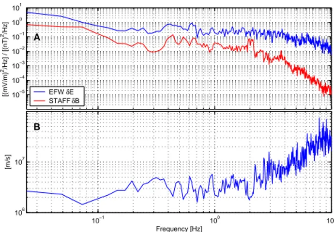
the cusp for frequencies below the proton gyrofrequency is close to the Alfv´en velocity while it increases with higher frequencies. This can be clearly seen in Fig. 2, where we
show a line spectra of the δE⊥/δB⊥-ratio calculated for a
time interval in the HLBL. Panel (a) shows the power spec-tral density of the wave electric field δE from C4, from the time interval 02:54:00–02:56:00 UT (blue line), and the cor-responding power spectral density of the magnetic field δB
from STAFF (red line). Panel (b) shows the ratio δE⊥/δB⊥.
The ratio stays constant when f →0 and is of the order of the local Alfv´en speed.
The polarization parameters for the magnetic field, as de-fined by Carozzi et al. (2001) were calculated in a field-aligned coordinate system and are presented for C4 in Fig. 3. We have chosen to present the polarization analysis in a field-aligned coordinate system rather than a minimum variance frame, since this representation is closer to a theoretical de-scription of possible wave modes. In a field-aligned coordi-nate system right or left handness can be inferred directly by calculating the polarization parameters of the perpendicular components. Figure 3a shows the power spectral density of the magnetic field as measured by FGM. The degree of polar-ization of the two magnetic field components perpendicular to the ambient magnetic field is shown in panel (b) while in panel (c), the ellipticity is shown for the same components. The degree of polarization is low and no definite polariza-tion in terms of right- or left handedness can be seen in the perpendicular plane.
If the same polarization analysis is carried out in the plane spanned by the ambient magnetic field direction and the sun-ward pointing perpendicular direction, a clear polarization is observed. For this case Fig. 3, panel (d), shows a higher de-gree of polarization for frequencies below and slightly above
fcp. The proton gyrofrequency is clearly visible in panel (e),
where the ellipticity changes sign from positive to negative, meaning that the sense of polarization changes direction in
10−5 10−4 10−3 10−2 10−1 100 101 [(mV/m) 2/Hz] / [(nT) 2/Hz] A EFW δE STAFF δB 10−1 100 101 106 107 Frequency [Hz] [m/s] B
Fig. 2. Panel (a) Power spectral density of the electric and
mag-netic field and panel (b) the δE⊥/δB⊥-ratio for the time interval
02:54:00–02:56:00 UT in the HLBL. In the low frequency limit the δE⊥/δB⊥-ratio is of the order of the Alfv´en velocity (1300–
1500 km/s). The proton gyrofrequency was ∼1.6 Hz.
this plane. If the sunward pointing perpendicular component is exchanged for the duskward perpendicular component, a higher degree of polarization is again observed, panel (f), though the ellipticity signature is not as evident in this case, panel (g). This feature of the polarization is consistent with
a change in sign of one component of k, i.e. either k⊥or kk
(see Discussion).
Examining hodograms of the magnetic field, Fig. 4, cor-responding to the projections used in Fig. 3, reveals the rea-son for the degree of polarization found. Figure 4a shows a hodogram representation of the perpendicular components from the wave magnetic field of C4, band-pass filtered
be-tween 1.0–1.5 Hz (below fcp). It is noticed that the
polariza-tion changes direcpolariza-tion on a time scale compared to the wave period. The time scale for change in the sense of polarza-tion is shorter than the time scale over which averaging is made for the spectrograms in Fig. 3, hence the low degree of polarization in this projection plane. Figures 4b and 4c shows hodogram representations for the two perpendicular vs. parallel projections. In this case the period for polariza-tion changes is longer, resulting in a higher degree of po-larization. The same kind of hodograms but now band-pass
filtered at 1.8–2.3 Hz (above fcp) are presented in panels (d),
(e) and (f). The same features are seen in this case, except that the sense of polarity has changed, panel (e).
2.5 Wave multi-spacecraft analysis
The short separation of the spacecraft allows for the uti-lization of multi-spacecraft techniques to gain information on wave properties. Figure 5 shows the configuration of the spacecraft with respect to the ambient magnetic field
at 03:00 UT. C1 and C2 are aligned almost along the
same field line. Their perpendicular separation was only 29 km, while their parallel separation was 76 km. No other pair of spacecraft was located so close to each other in the
[(nT) 2/Hz] −6 −4 −2 100 Hz A DOP 0.25 0.5 0.75 100 Hz B Ellipticity −1 0 1 100 Hz C DOP 0.25 0.5 0.75 100 Hz D Ellipticity −1 0 1 100 Hz E DOP 0.25 0.5 0.75 100 Hz F Ellipticity −1 0 1 02:55 03:00 100 Hz G
Fig. 3. Polarization in a field-aligned coordinate system as a function of frequency. Panel (a) shows the Fourier transform spectrogram of the
FGM magnetic field. Panel (b) shows the degree of polarization and panel (c) the ellipticity for the perpendicular components. Similarly for the sunward-pointing perpendicular and the parallel components in panels (d) and (e). Finally, panels (f) and (g) shows the same parameters for the duskward-pointing perpendicular and the parallel components.
−0.2 −0.1 0 0.1 0.2 0.3 −0.2 −0.1 0 0.1 0.2 perp1 perp2 02:54:29−02:54:31UT. 1.0−1.5Hz A −0.2 −0.1 0 0.1 0.2 0.3 −0.2 −0.1 0 0.1 0.2 perp1 parallel B −0.2 −0.1 0 0.1 0.2 0.3 −0.2 −0.1 0 0.1 0.2 perp2 parallel C −0.2 −0.1 0 0.1 0.2 0.3 −0.2 −0.1 0 0.1 0.2 perp1 perp2 02:54:30−02:54:31UT. 1.8−2.3Hz D −0.2 −0.1 0 0.1 0.2 0.3 −0.2 −0.1 0 0.1 0.2 perp1 parallel E −0.2 −0.1 0 0.1 0.2 0.3 −0.2 −0.1 0 0.1 0.2 perp2 parallel F
Fig. 4. Hodograms of the wave magnetic field from C4 in a
field-aligned coordinate system, filtered in two different frequency inter-vals below and above fcp, respectively. The square marks the start
of the time series, and the circle the end.
perpendicular direction. On the other hand, e.g. the pair C1-C4 was separated 43 km in parallel direction, roughly half the parallel distance of the pair C1-C2, and 63 km in the per-pendicular direction. For comparison, the proton gyroradius
was approximately ρp∼23 km (calculated for a mean energy
of 300 eV, see Fig. 1a).
We show the results of a cross-spectral analysis using the sunward pointing perpendicular component of the
mag-netic field. Similar results are obtained using the other
components. The cross-spectrum of two time signals, si and
sj, is defined by (e.g. Labelle and Kintner, 1989)
Cij(ω) = SiSj∗ q |Si|2 |Sj|2 =γ (ω)2ei1θij(ω), (1)
where Si and Sj are the Fourier transform of si and sj,
re-spectively, and angle brackets represent ensamble averages. In practice, the ensamble average is realized by taking time averages with a window of suitable length, due to the inher-ent problem of observing the same physical process with re-peated observations in satellite measurements. The
ampli-tude γ2denotes the coherency of the cross-spectrum, while
1θijis the phase.
Figure 6 shows an example of a cross-spectral analysis of signals from the pairs C1-C2 and C1-C4, respectively; the examples are from HLBL region. The coherency, Fig. 6b, is
high in a large frequency band centered around fcp for the
pair C1-C2 (red line). In panel (c) the phase difference be-tween the signals is plotted as a function of frequency. There is a clear trend in phase difference in a wide frequency range
around fcp (red crosses). This indicates that these waves
most probably satisfy the same dispersion relation and in addition, it can be seen that 2π wrapping is not involved. The relation between phase and frequency in the frequency
interval around fcp results in a phase velocity projected on
the spacecraft separation axis dij. For a plane wave the
phase difference between two spatially separated points (two spacecraft) is given by
-50 0 50 L [km] -50 0 50 -50 0 50 N [km] M [km] L=[ -0.34 -0.15 -0.93] GSE N=[0.94 -0.06 -0.34] M=[0.00 -0.99 0.16] C1 C2 C3 C4
Fig. 5. Location of the Cluster spacecraft corresponding to Fig. 6.
L, M and N are the parallel and two perpendicular axes, respec-tively, in a field-aligned coordinate system. L is the field-aligned direction, N is the perpendicular component pointing towards the Sun, and M completes the right-handed system. At this time C1 and C2 are at the smallest perpendicular separation and hence al-most on the same field line.
where k·dij=kijdij is the projection of the k-vector on the
interferometer axis. This gives the phase velocity along the interferometer axis vph,ij = 2πf kij = 2πf 1θij/dij . (3)
Here 1θij in Eqs. (2), (3) is the same as in Eq. (1). Using
values from Fig. 5 and Fig. 6 results in a projected phase
ve-locity of approximately vph,(C1−C2)∼250–300 km/s. Since
kij≤k always holds true, the phase velocity estimate along
the interferometry axis is an upper bound on the true phase velocity, i.e. vph≤vph,ij.
The separation axis is mostly along the parallel direction, which, at first sight, seems to imply that the obtained value of the projected phase velocity is a good estimate of a parallel phase velocity. However, this is true only if the phase veloc-ity of the wave is almost parallel with respect to the ambient
magnetic field, i.e. kk>k⊥. If the phase velocity is almost
perpendicular, k⊥>kk, then even though the separation axis
is close to being parallel with respect to the ambient magnetic field, the parallel phase velocity and phase velocity along the separation axes can differ significantly. In this case one can still use the phase velocity along the separation axis to es-timate the perpendicular phase velocity. There is additional information that allows us to speculate that the waves in our
case satisfy the condition k⊥ kk.
02:54:00 02:54:20 02:54:40 02:55:00 02:55:20 02:55:40 02:56:00 −35 −30 −25 [nT] A 0 0.5 1 1.5 2 2.5 3 3.5 4 4.5 5 0 0.5 1 frequency [Hz] coherency B 0 0.5 1 1.5 2 2.5 3 3.5 4 4.5 5 −200 −100 0 100 200 frequency [Hz] phase difference C
Fig. 6. Cross spectral analysis of the sunward-pointing
perpendicu-lar magnetic field component for the spacecraft pairs C1-C2 which were situated almost along the same field line, and C1-C4 which had a larger perpendicular separation but a closer parallel separation. (a) Time series of the magnetic field. Black, red and blue are C1, C2 and C4, respectively. C2 and C4 have been shifted by –3 nT and +3 nT, respectively, for clarity. (b) Coherency from cross-spectral analysis. Red from the pair C1-C2, and blue from C1-C4. (c) Phase difference between the signals. The different markers corresponds to points with γ2≥0.5 (crosses) or γ2<0.5 (dots). Colors as in panel (b).
In Sect. 2.3, Fig. 1c, we showed that the Poynting flux
changes direction at fcp, which for wave modes where the
parallel group velocity is in the same direction as the
par-allel phase velocity implies that kkshould also change sign
at fcp. This is not observed in Fig. 6c. The slope is about
the same above and below fcp, although a jump in the slope
is observed. This is consistent with the Poynting flux
re-sults, if k⊥ kk holds true. The measured phase difference
will then be an estimate of a perpendicular phase
veloc-ity, since k·d=(k⊥+kk)·d≈k⊥·d. The effect of kk
chang-ing sign at fcp will still be notable as a discontinuous jump
in the phase difference versus frequency diagram, as is ob-served in Fig. 6c. Since the perpendicular separation is about
2–3 times smaller compared to d12, vph,(C1−C2) will be an
upper bound, and the final estimate of vph,⊥is of the order of
vph,⊥∼100 km/s. We note that this phase velocity has been
calculated in the spacecraft frame of reference, and that a possible Doppler shift could alter the value in the plasma rest frame. This phase velocity is much smaller than the Alfv´en velocity. Small phase velocities are observed regardless of whether the spacecraft are located in the HLBL or the cusp proper in this event. The phase velocity in the frequency in-terval 1–2 Hz also gives an upper bound estimate of the
per-pendicular wavelength λ⊥∼50–100 km.
The same kind of analysis is presented for the pair C1-C4 with blue lines and markers in Fig. 6. One of the space-craft (C1) is the same in these two pairs. As is evident from panel (b) there is almost no coherency between the signals of
A B C
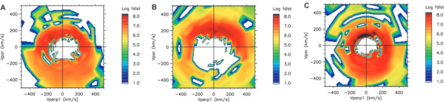
Fig. 7. Proton distribution functions from C4, showing shell-like features. (a) 02:54:59 UT, (b) 02:56:58 UT, (c) 03:09:58 UT. Shown is
distribution function cuts in parallel and one perpendicular direction. Cuts of the distribution functions in perpendicular-perpendicular plane also display similar features (not shown).
C1 and C4. The points in phase-frequency space, panel (c), do not align along a line but are randomly distributed. The perpendicular separation of C1 and C4 is ∼60 km, while the parallel separation is ∼40 km. Thus, we observe no co-herency for these emissions when the inter-spacecraft sepa-ration is smaller in parallel but longer in the perpendicular direction than for the pair C1-C2. Similarly low coherence is observed for all spacecraft pairs except the pair C1-C2, for all other times, for this boundary crossing. In summary, good coherency is only observed when the spacecraft are aligned almost along the same field line, and measured phase veloci-ties are almost one order of magnitude lower than the Alfv´en velocity. Since the perpendicular separation of all pair of spacecraft is greater than for the pair C1-C2, even though the parallel separation could be smaller, we draw the following conclusions:
– The wave emissions around the proton gyrofrequency observed on all four spacecraft have a coherence length
of at least 80 km (&4ρp)in parallel direction, and at
least 30 km but at most 60 km (1–3ρp) in the
perpendic-ular direction.
– Measured perpendicular phase velocities are of the or-der of 100 km/s, an oror-der of magnitude lower than the Alfv´en velocity.
– The phase velocity estimate gives an upper bound of the
perpendicular wavelength λ⊥.50–100 km.
2.6 Ion distribution functions
In Fig. 7 we show the ion distribution functions from C4 for three different time intervals. All panels show cuts in the parallel-perpendicular plane. Panels (a) and (b) are distribu-tion funcdistribu-tions from two different times in the HLBL. Panel (b) clearly shows the proton injection around 02:58 UT that is mentioned in Sect. 2.1. The distribution functions resem-bles a horse-shoe shape. Such distribution functions, formed due to mirroring of downgoing ions in the converging mag-netic field, is expected to be present on recently reconnected field lines. Panel (c) shows an example of a distribution func-tion from the cusp proper. It can be seen that the distribufunc-tion
function is more symmetric than in panels (a) and (b). This is consistent with these field lines being reconnected for a longer time so that the injected plasma has had time to mir-ror and thus form a more symmetric distribution function. In the plasma frame (approximately equal to the ion center of mass reference frame) the distributions have a positive
gradi-ent ∂f/∂vk, ∂f/∂v⊥>0, for velocities around 100–200 km/s.
This is close to the estimated phase velocity of the waves and indicates that ions can be a free energy source of the waves as speculated below in the Discussion section.
3 Discussion
3.1 Wave properties
Our objective is to interpret the above described observations using known theoretical concepts. To this end we initially analyze the observational facts in terms of linear waves in a homogeneous plasma. Later, we give arguments as to why the theoretical model must be extended to include nonlinear and inhomogeneous effects.
In Sect. 2.4 we found that the δE⊥/δB⊥-ratio is of the
or-der of the local Alfv´en velocity in the low frequency limit. Together with the fact that we observe wave emissions both
below and above the local fcpsuggests that these waves can
be ion-whistlers (other names for this wave mode are com-pressional Alfv´en waves or magnetosonic waves), which can
exist both below and above fcp. We performed a preliminary
analysis of the wave properties using the Wave Distribution Function (WDF) technique (Oscarsson, 1994), that is based on a homogeneous plasma model. Parameters of the model were taken to correspond to real particle observations and real field parameters observed. We found that one can fit the data but only if we used rather large adjustments of the model parameters.
To give a better description of the waves we investigated what information single- and multiple-spacecraft measure-ments, such as polarization analysis and cross-correlation analysis, could provide (Sects. 2.4 and 2.5).
From the multi-spacecraft cross-spectral analysis (Sect. 2.5) we concluded that the phase velocity projected on the C1-C2 separation axis should be lower than ∼300 km/s and we argued that the most probable wave vector is almost perpendicular with respect to the ambient magnetic field
(k⊥ kk), in which case the perpendicular phase velocity
would be even lower, vph,⊥.100 km/s. This is an
or-der of magnitude lower than the Alfv´en speed obtained
from background parameters, vA∼1300–1500 km/s. The
phase velocity also gave an upper bound estimate of the
perpendicular wavelength λ⊥.50–100 km.
The multi-spacecraft analysis reveals another feature of these waves. As shown in Sect. 2.5 the coherence length is at least 80 km in a direction parallel to the ambient mag-netic field, and 30–60 km in the perpendicular direction. The relation between coherence length and wavelength is not triv-ial. However, as long as the wavelength is long compared to the interferometer axis, the coherency is large, even if the k-spectrum is broad (see Kintner et al., 2000). Thus the low coherency in the perpendicular direction gives an up-per bound estimate of the up-perpendicular length scale. The coherence length of 30–60 km corresponds to a
perpendicu-lar length scale of the order of one to three ρp(ρp∼23 km),
in agreement with the estimated characteristic wavelength above. This result is valid for frequencies both below and above fcp.
No clear polarization could be found between the perpen-dicular wave components, e.g. right-hand polarization would be expected for ion-whistlers (e.g. Stix, 1992). However, a clear polarization signature was observed between the par-allel component and the one perpendicular component. We noted that the ellipticity in this plane changes sign (sense of rotation) at the local fcp. Such a change in ellipticity would
be observed if for a given wave either k⊥ or kk changed
the sign. Note that in the perpendicular plane waves keep their polarization, e.g. whistlers are right-handed waves in-dependent of propagation direction. In Sect. 2.5 we argued
that indeed kkchanges sign at fcpand thus this is consistent
with the observed change of wave polarization in the plane
spanned by parallel-perpendicular directions at the local fcp
(Fig. 3). This also suggests that the waves below and above
fcpshould have very similar polarization properties, for
ex-ample, by being the same plasma wave mode.
First we look at waves with frequencies below fcp.
The electron inertial length c/ωpe∼3 km and the
elec-tron gyroradius ρe∼0.3 km are both much less than the
the ion-gyroradius ρp. Together with the fact that
me/mp βe∼0.01−0.04 1, this suggests that the waves
below fcpcan be identified as kinetic Alfv´en waves (KAW).
In a homogeneous plasma using thermal electrons, thermal ions and including finite frequency effects, the dispersion
re-lation of KAW for frequencies below fcp is (e.g. Stasiewicz
et al., 2000) ω2=kk2vA2 " 1 + k⊥2(ρs2+ρp2) − ω 2 ω2 cp (1 + k⊥2ρp2) # , (4) where ρs=p(Te/mp)/ωcp.
In the frequency range above fcp the short characteristic
perpendicular scale imposes certain constraints on possible wave modes. The perpendicular component for these waves should be of the order or even larger than the inverse ion-gyroradius k⊥&ρ−1
p . This excludes ion-whistlers
(compres-sional Alfv´en waves) as the only present wave mode, since WHAMP (R¨onnmark, 1982) calculations with the present plasma parameters show that the perpendicular wavelength for ion-whistlers is at least one order of magnitude longer than the observed coherence lengths. We cannot, however, exclude ion-whistlers altogether based on the length scale. A small part of the wave power could be due to whistler waves, but the dominant part should be due to another wave mode.
The measured perpendicular scale, together with the fact that these waves have a non-negligible magnetic field com-ponent, results in the identification of these waves as quasi-transverse propagating, non-potential ion-cyclotron waves. There exist several ion-cyclotron modes for quasi-transverse propagation: quasi-longitudinal, ordinary and extra-ordinary. Another name for these modes could be electromagnetic ion-Bernstein modes, although the label ion-ion-Bernstein is usually associated with the longitudinal (electrostatic) mode (see e.g. Akhiezer et al., 1975; Lominadze, 1981). It is worth noting the presence of peaks in the spectrum of the magnetic field near fcp, suggesting the presence of Bernstein waves. The non-potential ordinary modes couple to the kinetic Alfv´en waves around the cyclotron frequency for short perpendic-ular wavelengths, while the extra-ordinary mode couples to the ion-whistler wave (compressional Alfv´en). The
polariza-tion analysis suggested that waves below and above fcphave
the same polarization properties, which suggests that the
rel-evant modes above fcpare the quasi-longitudinal and/or
or-dinary ion-cyclotron modes.
We have used the coherence lengths as a means of gaining information on scale lengths. In general, the short perpendic-ular coherence length makes wave-mode identification diffi-cult. If good coherency is found between spacecraft for all spacecraft combinations, then a three-dimensional k can be determined, assuming a one-to-one correspondence between wave number and frequency. However, coherence lengths shorter than the spacecraft separation makes this impossi-ble. No 3-D k can be determined with phase difference tech-niques due to bad coherency for some spacecraft pairs. For the same reason k-filtering cannot be applied.
Up to now we have considered linear waves in a homoge-neous plasma. We present arguments why we probably must relax one or both of the constraints of linearity and homo-geneity, in order to describe the waves with sufficient accu-racy:
– Energetics: The ratio of energy fluxes in waves and
ions is PF/IPF∼2.5·10−2 for waves with frequencies
f ∼fcp. This suggests that a significant part of the
avail-able energy is in the waves and that nonlinear effects can be important.
02:54:00 2 02:54:20 02:54:40 02:55:00 02:55:20 02:55:40 02:56:00 2.5 3 3.5 4 4.5 5 09−Mar−2002 Density [cm¯³] C1 C2 C3
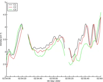
Fig. 8. Density estimates from EFW spacecraft potential
measure-ments (see Pedersen et al., 2001, for a general description of the method). The data gaps are due to instrumental interference from WHISPER. For example, at 02:55:40 UT, C3 measures a differ-ent density compared to C1 and C2. This implies a local density gradient of 25% on the length scale of the spacecraft separation ∼50 km (2ρp).
– Density gradients: Examining the density measured by different spacecraft at the same instant of time reveals that the plasma is inhomogeneous on the scale of the inter-spacecraft distances. The density can differ by
as much as 25% over a distance of ∼50 km (2ρp), see
Fig. 8.
Strong gradients on the scale of the ion-gyroradius, which is also the perpendicular wavelength, suggests that not only inhomogeneous but also nonlinear features must be taken into account. For example, for waves with frequencies
be-low fcp this means that Eq. (4) must be extended to include
nonlinearities and gradient (drift) effects. In this case non-linear drift Alfv´en waves can probably give a better descrip-tion, as they are known to create field-aligned electromag-netic structures in the form of vortices which could explain the observed emissions, polarization and coherence lengths (see, e.g. Shukla et al., 1985; Chmyrev et al., 1988; Dubinin et al., 1988). To explore in more detail all these possibilities is a topic of our future work.
3.2 Wave-particle interaction
The Poynting flux along the ambient magnetic field as a function of frequency shows two important features (see,
Sect. 2.3). First, below fcp the Poynting flux is
predomi-nantly downward (earthward) while it is mainly upward for
frequencies above fcp. This is consistent with a model where
waves are generated with frequencies close to the local pro-ton gyrofrequency in an extended region along the mag-netic field line. If these waves propagate both upward and downward from the generation site, then the waves with
frequencies below the local proton gyrofrequency are ex-pected to come from above where their frequency comes close to the local proton gyrofrequency and vice versa for waves above the proton gyrofrequency. Secondly, the net Poynting flux for these waves is small in comparison to the Poynting flux carried by lower frequency waves, except in HLBL, where they are comparable. Thus, the waves with frequencies around the proton gyrofrequency cannot trans-port significant energy in the cusp while they still can be important for particle energization and energy redistribution through wave-particle and wave-wave interaction. Similar observations have been reported from the auroral zone (Chas-ton et al., 1998, 2002). In regions of auroral particle acceler-ation with upward current these studies reported electromag-netic waves at the proton cyclotron frequency and its har-monics, unstable to both electron as well as ion beams. The
Poynting flux was found to be mainly upward above fcpand
downward below, similar to our findings.
We observe a correspondence between the electromag-netic waves and the presence of protons (see, Sect. 2.2). The fact that the ion power flux is approximately 40 times
larger than the Poynting flux for frequencies around fcp,
and that proton thermal velocities are of the order of wave phase velocities, makes it plausible that the protons are the source of free energy for the waves. Cluster also observes anisotropic electrons at the same time as the waves and pro-tons. Preliminary analysis of electron power flux does not allow us to draw any conclusions about the possibility of electrons being the free energy source of waves; more care must be taken to reduce instrumental uncertainties. On the other hand, the electron distribution functions seem to indi-cate that electrons can be locally accelerated along the mag-netic field lines to Alfv´en speeds. This would be consistent with earlier studies (Hasegawa, 1976; Stasiewicz et al., 2000, and references therein) suggesting that anisotropic electron distribution functions can be due to acceleration by kinetic Alfv´en waves. We leave the thorough analysis of electrons and the coupling between low-frequency Alfv´en waves and high-frequency electron waves to our future study.
To identify the source of free energy we examined the pro-ton distribution functions in Sect. 2.6. We found ion shell distributions with ion velocities at the location of the positive derivatives around ∼100–200 km/s, close to our estimates of the phase velocities of the waves. Ion shell distributions are known to generate, e.g. ion-Bernstein waves (Janhunen et al., 2003), while 2-D analogue ring distributions are known to generate, e.g. ion-whistlers (Perraut et al., 1982; Korth et al., 1984), and thus is a plausible source of the waves.
To investigate more quantitatively if the proton shell dis-tributions can be the source of the waves we modeled the observed particle distributions in WHAMP. The proton shell was modeled by adding two Maxwellian distributions for
the protons with characteristic parameters (Tp1=400 eV,
np1=4 cm−3) and (Tp2=130 eV, np1=–0.8 cm−3). The
sec-ond distribution has a negative density, in order to make the resulting distribution resemble a shell. The electrons were modeled by a single Maxwellian distribution with the
parameters (Te=130 eV, np1=3.2 cm−3). The output is
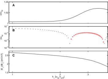
pre-sented in Fig. 9, which shows the first ion cyclotron
har-monic for a value of k||=0.1ωcp/vp,t h. Panels (a) and (b)
shows the real (ω) and imaginary parts (γ ) of the frequency, respectively, plotted as a function of k⊥. We note that
in-deed considerable wave growth (γ ∼10−2ωcp, with a
max-imum of γ =0.08 fcp=0.13 s−1) occurs for perpendicular
wavelengths λ⊥'1.5 ρp, where we have used vp,t h∼300 eV,
k⊥=3 ωcp/vp,t h and fcp=1.6 Hz. This is in good
agree-ment with the observed wavelengths obtained from the
multi-spacecraft cross-spectral analysis above (λ⊥∼1-4 ρp). The
E⊥/B⊥-ratio is plotted in panel (c), indicating the
non-potential (magnetic component) nature of the waves. This ratio is in agreement with Fig. 2. We finally note that since the electrons are Maxwellian, they do not contribute to the observed wave growth in our model. Modeling the distribu-tions more carefully and investigating other wave modes than ion cyclotron waves is a topic we leave for a future study.
There are other possible free energy sources that we have not discussed in detail here. For example, one such source can be shear velocity flows in the plasma that are often ob-served in the cusp and its boundary layers and are also seen in our event. In addition, large-scale currents, such as diamag-netic currents, can be a source of free energy. The magdiamag-netic field spectrum shows a combination of a spectral peak around
fcpand a broad-band spectra with different slopes below and
above fcp(Fig. 2), which also indicate a possibility of
hav-ing several wave sources. Kinked double slope spectra in the cusp has also been previously reported from Interball-1 and Polar observations (Savin et al., 2002).
In summary, ion power flux, the Poynting flux distribution
over frequency, peaks at fcpand its multiples, together with
the proton shell distribution functions and sheared plasma flow, make it probable that the waves are generated locally in the cusp along the field lines, from one or possibly more sources by an instability which favours the ion-cyclotron fre-quency.
4 Summary and conclusions
We have done a detailed study of waves with frequencies near the proton gyrofrequency in the high-altitude cusp for north-ward IMF as observed by the Cluster spacecraft. Our main conclusions are:
– All four spacecraft observe enhanced emissions in the electric and magnetic fields both below and above the
proton gyrofrequency. The emissions are most
pro-nounced at the poleward edge of the cusp in localized regions of injected 300 eV ions. The injected ions are most probably caused by the reconnection at the mag-netopause tailward (higher latitude side) of the cusp as expected for the observed northward IMF.
– Single spacecraft measurements of the δE⊥/δB⊥-ratio show that the waves are electromagnetic with a
1 1.02 1.04 ω / ωcp A 10−4 10−3 10−2 10−1 γ / ωcp B 1 2 3 1.5 2 2.5 k⊥ [ωcp/vp,th] |E⊥ |/|B ⊥ | [mV/nT] C
Fig. 9. Ion cyclotron mode obtained from WHAMP with proton
shell and Maxwellian electron distributions modeled from particle measurements. (a) Frequency vs. perpendicular wavenumber. (b) Imaginary part of frequency vs. perpendicular wave number. Black dots stand for γ <0 (damping) and red crosses for γ >0 (growth). (c) E⊥/B⊥-ratio. The parallel wave number was k||=0.1ωcp/vp,t h.
δE⊥/δB⊥-ratio of the order of the local Alfv´en speed
in the low frequency limit.
– There is a low degree of polarization in the plane perpendicular to the ambient magnetic field, due to a change in the sense of rotation on a time scale compa-rable to the wave period. However, there is a clear po-larization in one parallel-perpendicular plane. A change in the sense of polarization in the parallel-perpendicular
plane is consistent with a change in the sign of kkwith
respect to fcp.
– The measurements are consistent with k⊥ kk. Cross-spectral analysis of the wave magnetic field between spacecraft results in an estimate of the perpendicular phase velocity of the order of 100 km/s, which is much
less than the local Alfv´en speed vA∼1300–1500 km/s.
From the phase velocity follows that the perpendicular wavelength should be a few proton gyroradius or less,
λ⊥.2–4ρp.
– The waves have a coherence length which is of the or-der of one ion-gyroradius in the direction perpendicular to the ambient magnetic field and a few times larger or more in the parallel direction.
– The coherence length gives an upper bound for a per-pendicular wavelength or length scale of the order of the ion-gyroradius, agreeing in order with the estimated wavelength. This gives constraints on possible wave modes and implies that kinetic (finite gyroradius) ef-fects are important.
– Below fcp the waves supposedly belong to the kinetic
waves are the most probable wave mode which can cou-ple to the kinetic Alfv´en wave around the cyclotron fre-quency for short perpendicular wavelengths.
– Large plasma density gradients are observed on the scale of perpendicular wavelengths (on the order of the ion-gyroradius), which suggest that nonlinear and non-homogeneous effects are important.
– The Poynting flux projected on the ambient magnetic field is mainly downward (earthward) below the local
fcp, and upward above the local fcp. This feature of the
Poynting flux is consistent with the waves being gener-ated near the local proton gyrofrequency in an extended region along the flux tube.
– A likely source of free energy driving the waves with
frequencies around fcp are injected protons. First, the
observed waves show a correspondence to the proton flux. Secondly, the calculated ion power flux is approx-imately 40 times larger than the wave Poynting flux. Fi-nally, the injected protons show shell-like distribution functions that have positive gradients and are thus ki-netically unstable; the velocity at the positive gradients is of the order of the measured phase velocity of waves. Linear wave growth calculations using WHAMP sup-ports this picture by showing significant wave growth at perpendicular wavelengths agreeing with measure-ments.
Here we have shown that multipoint measurements are es-sential for studying waves in the cusp and its boundaries. In our future work we believe that it is important to look at wave models extended to include either nonlinearities and/or inho-mogeneities on scales of the order of the ion-gyroradius, as well as velocity shear effects.
Acknowledgements. D. Sundkvist and V. Krasnoselskikh
acknowl-edge financial support from the European Community’s Human Po-tential Programme under contract HPRN-CT-2001-00314 “Turbu-lent Boundary Layers in Geospace Plasmas”.
D. Sundkvist also wish to thank GradU, Uppsala University, for fi-nancial support, and A. Tjulin for useful discussions.
A. Vaivads research is supported by the Swedish Research Council. Topical Editor T. Pulkkinen thanks J. Blecki and C. Chaston for their help in evaluating this paper.
References
Akhiezer, A. I., Akhiezer, I. A., Polovin, R. V., Sitenko, A. G., and Stepanov, K. N.: Plasma Electrodynamics, Volume 1: Linear Theory, Pergamon Press, 1975.
Andr´e, M.: Waves and wave-particle interactions in the auroral re-gion, J. Atmos. Terr. Phys., 59, 1687–1712, 1997.
Andr´e, M., Koskinen, H., Gustafsson, G., and Lundin, R.: Ion waves and upgoing ion beams observed by the Viking satellite, Geophys. Res. Lett., 14, 463–466, 1987.
Andr´e, M., Norqvist, P., Andersson, L., Eliasson, L., Eriksson, A. I., Blomberg, L., Erlandson, R. E., and Waldemark, J.: Ion ener-gization mechanisms at 1700 km in the auroral region, J. Geo-phys. Res., 103, 4199–4222, 1998.
Balogh, A., Dunlop, M. W., Cowley, S. W. H., Southwood, D. J., Thomlinson, J. G., Glassmeier, K. H., Musmann, G., Luhr, H., Buchert, S., Acu˜na, M. H., Fairfield, D. H., Slavin, J. A., Riedler, W., Schwingenschuh, K., and Kivelson, M. G.: The Cluster Mag-netic Field Investigation, Space Sci. Rev., 79, 65–91, 1997. Bouhram, M., Malingre, M., Jasperse, J. R., and Dubouloz, N.:
Modeling transverse heating and outflow of ionospheric ions from the dayside cusp/cleft. 1 A parametric study, Ann. Geo-phys., 21, 1753–1771, 2003a,
SRef-ID: 1432-0576/ag/2003-21-1753.
Bouhram, M., Malingre, M., Jasperse, J. R., Dubouloz, N., and Sauvaud, J.-A.: Modeling transverse heating and outflow of ionospheric ions from the dayside cusp/cleft. 2 Applications, Ann. Geophys., 21, 1773–1791, 2003b,
SRef-ID: 1432-0576/ag/2003-21-1773.
Carozzi, T. D., Thid´e, B., Leyser, T. B., Komrakov, G., Frolov, V., Grach, S., and Sergeev, E.: Full polarimetry measurements of stimulated electromagnetic emissions: First results, J. Geophys. Res., 21 395–21 408, 2001.
Chaston, C. C., Ergun, R. E., Delory, G. T., Peria, W., Temerin, M., Cattell, C., Strangeway, R., McFadden, J. P., Carlson, C. W., El-phic, R. C., Klumpar, D. M., Peterson, W. K., Moebius, E., and Pfaff, R.: Characteristics of electromagnetic proton cyclotron waves along auroral field lines observed by FAST in regions of upward current, Geophys. Res. Lett., 25, 2057–2060, 1998. Chaston, C. C., Bonnell, J. W., McFadden, J. P., Ergun, R. E., and
Carlson, C. W.: Electromagnetic ion cyclotron waves at proton cyclotron harmonics, J. Geophys. Res., 107, 8–1, 2002. Chmyrev, V. M., Bilichenko, S. V., Pokhotelov, O. A., Marchenko,
V. A., Lazarev, V. I., Streltsov, A. V., and Stenflo, L.: Alfv´en Vor-ticies and Related Phenomena in the Ionosphere and the Magne-tosphere, Physica Scripta, 38, 841–854, 1988.
Cornilleau-Wehrlin, N., Chauveau, P., Louis, S., Meyer, A., Nappa, J. M., Perraut, S., Rezeau, L., Robert, P., Roux, A., de Villedary, C., de Conchy, Y., Friel, L., Harvey, C. C., Hubert, D., La-combe, C., Manning, R., Wouters, F., Lefeuvre, F., Parrot, M., Pincon, J. L., Poirier, B., Kofman, W., and Louarn, P.: The Clus-ter Spatio-Temporal Analysis of Field Fluctuations (STAFF) Ex-periment, Space Sci. Rev., 79, 107–136, 1997.
Dubinin, E. M., Volokitin, A. S., Israelevich, P. L., and Niko-laeva, N. S.: Auroral electromagnetic disturbances at altitudes of 900km: Alfv´en wave turbulence, Planet. Space Sci., 36, 949– 962, 1988.
Erlandson, R. E. and Zanetti, L. J.: A statistical study of auro-ral electromagnetic ion cyclotron waves, J. Geophys. Res., 103, 4627–4636, 1998.
Fredricks, R. W. and Russell, C. T.: Ion cyclotron waves observed in the polar cusp, J. Geophys. Res., 78, 2917, 1973.
Gurnett, D. A.: Auroral Plasma Waves, in Auroral Physics, edited by: Meng, C.-I., Rycroft, M. J., and Frank, L. A., Cambrige University Press, Cambridge, UK, 241–245, 1991.
Gurnett, D. A. and Frank, L. A.: A region of intense plasma wave turbulence on auroral field lines, J. Geophys. Res., 82, 1031– 1050, 1977.
Gustafsson, G., Andr´e, M., Matson, L., and Koskinen, H.: On waves below the local proton gyrofrequency in auroral accelera-tion regions, J. Geophys. Res., 95, 5889–5904, 1990.
Gustafsson, G., Bostr¨om, R., Holback, B., Holmgren, G., Lundgren, A., Stasiewicz, K., ˚Ahl´en, L., Mozer, F. S., Pankow, D., Har-vey, P., Berg, P., Ulrich, R., Pedersen, A., Schmidt, R., Butler, A., Fransen, A. W. C., Klinge, D., Thomsen, M., F¨althammar, C.-G., Lindqvist, P.-A., Christenson, S., Holtet, J., Lybekk, B.,
Sten, T. A., Tanskanen, P., Lappalainen, K., and Wygant, J.: The Electric Field and Wave Experiment for the Cluster Mission, Space Sci. Rev., 79, 137–156, 1997.
Hamrin, M., Norqvist, P., Hellstr¨om, T., Andr´e, M., and Eriksson, A. I.: A statistical study of ion energization at 1700 km in the auroral region, Ann. Geophys., 20, 1943–1958, 2002,
SRef-ID: 1432-0576/ag/2002-20-1943.
Hasegawa, A.: Particle acceleration by MHD surface wave and for-mation of aurora, J. Geophys. Res., 81, 5083–5090, 1976. Janhunen, P., Olsson, A., Vaivads, A., and Peterson, W. K.:
Gener-ation of Bernstein waves by ion shell distributions in the auroral region, Ann. Geophys., 21, 881–891, 2003,
SRef-ID: 1432-0576/ag/2003-21-881.
Johnstone, A. D., Alsop, C., Burge, S., Carter, P. J., Coates, A. J., Coker, A. J., Fazakerley, A. N., Grande, M., Gowen, R. A., Gur-giolo, C., Hancock, B. K., Narheim, B., Preece, A., Sheather, P. H., Winningham, J. D., and Woodliffe, R. D.: Peace: a Plasma Electron and Current Experiment, Space Sci. Rev., 79, 351–398, 1997.
Kaufmann, R. L. and Kintner, P. M.: Upgoing ion beams, I – Mi-croscopic analysis, J. Geophys. Res., 87, 10 487–10 502, 1982. Kintner, P. M., Franz, J., Schuck, P., and Klatt, E.: Interferometric
coherency determination of wavelength or what are broadband ELF waves?, J. Geophys. Res., 105, 21 237–21 250, 2000. Korth, A., Kremser, G., Perraut, S., and Roux, A.: Interaction of
particles with ion cyclotron waves and magnetosonic waves. Ob-servations from GEOS 1 and GEOS 2, Planet. Space Sci., 32, 1393–1406, 1984.
Labelle, J. and Kintner, P. M.: The measurement of wavelength in space plasmas, Rev. Geophys., 27, 495–518, 1989.
Le, G., Blanco-Cano, X., Russell, C. T., Zhou, X.-W., Mozer, F., Trattner, K. J., Fuselier, S. A., and Anderson, B. J.: Electro-magnetic ion cyclotron waves in the high altitude cusp: Polar observations, J. Geophys. Res., 106, 19 067–19 079, 2001. Lominadze, D. G.: Cyclotron Waves in Plasma, Pergamon Press,
1981.
Nykyri, K., Cargill, P. J., Lucek, E. A., Horbury, T. S., Balogh, A., Lavraud, B., Dandouras, I., and R`eme, H.: Ion cyclotron waves in the high altitude cusp: CLUSTER observations at vary-ing spacecraft separations, Geophys. Res. Lett., 30, 12–1, 2003. Nykyri, K., Cargill, P. J., Lucek, E., Horbury, T., Lavraud, B.,
Balogh, A., Dunlop, M. W., Bogdanova, Y., Fazakerley, A., Dan-douras, I., and R`eme, H.: Cluster observations of magnetic field fluctuations in the high-altitude cusp, Ann. Geophys., 22, 2413– 2429, 2004,
SRef-ID: 1432-0576/ag/2004-22-2413.
Oscarsson, T.: Dual principles in maximum entropy reconstruction of the wave distribution function, J. Comput. Ph., 110, 221–233, 1994.
Pedersen, A., D´ecr´eau, P., Escoubet, C.-P., Gustafsson, G., Laakso, H., Lindqvist, P.-A., Lybekk, B., Masson, A., Mozer, F., and Vaivads, A.: Four-point high time resolution information on elec-tron densities by the electric field experiments (EFW) on Cluster, Ann. Geophys., 19, 1483–1489, 2001,
SRef-ID: 1432-0576/ag/2001-19-1483.
Perraut, S., Roux, A., Robert, P., Gendrin, R., Sauvaud, J.-A., Bosqued, J.-M., Kremser, G., and Korth, A.: A systematic study of ULF waves above F/H plus/ from GEOS 1 and 2 mea-surements and their relationships with proton ring distributions, J. Geophys. Res., 87, 6219–6236, 1982.
R`eme, H., Bosqued, J. M., Sauvaud, J. A., Cros, A., Dandouras, J., Aoustin, C., Bouyssou, J., Camus, T., Cuvilo, J., Martz, C., Medale, J. L., Perrier, H., Romefort, D., Rouzaud, J., D‘Uston, C., Mobius, E., Crocker, K., Granoff, M., Kistler, L. M., Popecki, M., Hovestadt, D., Klecker, B., Paschmann, G., Scholer, M., Carlson, C. W., Curtis, D. W., Lin, R. P., McFadden, J. P., Formisano, V., Amata, E., Bavassano-Cattaneo, M. B., Baldetti, P., Belluci, G., Bruno, R., Chionchio, G., di Lellis, A., Shel-ley, E. G., Ghielmetti, A. G., Lennartsson, W., Korth, A., Rosen-bauer, H., Lundin, R., Olsen, S., Parks, G. K., McCarthy, M., and Balsiger, H.: The Cluster Ion Spectrometry (CIS) Experiment, Space Sci. Rev., 79, 303–350, 1997.
R¨onnmark, K.: Waves in homogeneous, anisotropic multicompo-nent plasmas (WHAMP), Tech. rep., KRI, 1982.
Russel, C. T., Chappell, C. R., Montgomery, M. D., Neugebauer, M., and Scarf, F. L.: Ogo 5 observations of the polar cusp on November 1, 1968, J. Geophys. Res., 76, 6743, 1971.
Santol´ık, O., Pickett, J. S., Gurnett, D. A., and Storey, L. R. O.: Magnetic component of narrowband ion cyclotron waves in the auroral zone, J. Geophys. Res., 107, 17–1, 2002.
Savin, S., Zelenyi, L., Maynard, N., Sandahl, I., Kawano, H., Rus-sell, C. T., Romanov, S., Amata, E., Avanov, L., Blecki, J., Buechner, J., Consolini, G., Gustafsson, G., Klimov, S., Mar-cucci, F., Nemecek, Z., Nikutowski, B., Pickett, J., Rauch, J. L., Safrankova, J., Skalsky, A., Smirnov, V., Stasiewicz, K., Song, P., Trotignon, J. G., and Yermolaev, Y.: Multi-spacecraft tracing of turbulent boundary layer, Adv. Space Res., 30, 2821–2830, 2002.
Savin, S., Zelenyi, L., Romanov, S., Sandahl, I., Pickett, J., Amata, E., Avanov, L., Blecki, J., Budnik, E., B¨uchner, J., Cattell, C., Consolini, G., Fedder, J., Fuselier, S., Kawano, H., Klimov, S., Korepanov, V., Lagoutte, D., Marcucci, F., Mogilevsky, M., Ne-mecek, Z., Nikutowski, B., Nozdrachev, M., Parrot, M., Rauch, J., Romanov, V., Romantsova, T., Russell, C., Safrankova, J., Sauvaud, J., Skalsky, A., Smirnov, V., Stasiewicz, K., Trotignon, J., and Yermolaev, Y.: Magnetosheath-cusp interface, Ann. Geo-phys., 22, 183–212, 2004,
SRef-ID: 1432-0576/ag/2004-22-183.
Scarf, F. L., Fredricks, R. W., Green, I. M., and Russell, C. T.: Plasma waves in the dayside polar cusp, 1, Magnetospheric ob-servations, J. Geophys. Res., 77, 2274, 1972.
Shukla, P. K., Yu, M. Y., and Varma, R. K.: Formation of kinetic Alfv´en vortices, Phys. Lett. A, 109, 322–324, 1985.
Stasiewicz, K., Bellan, P., Chaston, C., Kletzing, C., Lysak, R., Maggs, J., Pokhotelov, O., Seyler, C., Shukla, P., Stenflo, L., Streltsov, A., and Wahlund, J.-E.: Small Scale Alfv´enic Struc-ture in the Aurora, Space Sci. Rev., 92, 423–533, 2000. Stenberg, G., Oscarsson, T., Andr´e, M., and Chaston, C. C.:
Inves-tigating wave data from the FAST satellite by reconstructing the wave distribution function, J. Geophys. Res., 107, 19–1, 2002. Stix, T. H.: Waves in Plasmas, Am. Inst. of Phys., New York, 1992. Temerin, M. and Lysak, R. L.: Electromagnetic ion cyclotron mode (ELF) waves generated by auroral electron precipitation, J. Geo-phys. Res., 89, 2849–2859, 1984.
Wahlund, J.-E., Yilmaz, A., Backrud, M., Sundkvist, D., Vaivads, A., Winningham, D., Andr´e, M., Balogh, A., Bonnell, J., Buchert, S., Carozzi, T., Cornilleau, N., Dunlop, M., Eriksson, A. I., Fazakerley, A., Gustafsson, G., Parrot, M., Robert, P., and Tjulin, A.: Observations of auroral broadband emissions by CLUSTER, Geophys. Res. Lett., 30, 17–1, 2003.