HAL Id: inria-00436757
https://hal.inria.fr/inria-00436757
Submitted on 27 Nov 2009
HAL is a multi-disciplinary open access
archive for the deposit and dissemination of
sci-entific research documents, whether they are
pub-lished or not. The documents may come from
teaching and research institutions in France or
abroad, or from public or private research centers.
L’archive ouverte pluridisciplinaire HAL, est
destinée au dépôt et à la diffusion de documents
scientifiques de niveau recherche, publiés ou non,
émanant des établissements d’enseignement et de
recherche français ou étrangers, des laboratoires
publics ou privés.
Modeling and 3D local estimation for in-plane and
out-of-plane motion guidance by 2D ultrasound-based
visual servoing
R. Mebarki, A. Krupa, François Chaumette
To cite this version:
R. Mebarki, A. Krupa, François Chaumette. Modeling and 3D local estimation for in-plane and
out-of-plane motion guidance by 2D ultrasound-based visual servoing. IEEE Int. Conf. on Robotics and
Automation, ICRA’09, 2009, Kobe, Japan, Japan. pp.319-325. �inria-00436757�
Modeling and 3D local estimation for in-plane and out-of-plane motion
guidance by 2D ultrasound-based visual servoing
Rafik Mebarki, Alexandre Krupa and Franc¸ois Chaumette
Abstract— This paper presents a new model-free visual
ser-voing that is able to servo a robotized 2D ultrasound probe that interacts with a soft tissue object. It makes direct use of the B-mode ultrasound images in order to reach a desired one. This approach does not require the 3D model of the object nor its location in the 3D space. The visual features are based on image moments. The exact analytical form of the interaction matrix relating the image moments variation to the probe velocity is modelled. To perform model-free servoing, the approach combines the image points coordinates with the probe pose to estimate efficiently 3D parameters required in the control law. The approach is validated with simulation and experimental results showing its robustness to different errors and perturbations.
Index Terms— Visual servoing, ultrasound, model-free
con-trol, image moments, medical robotics.
I. INTRODUCTION
Image-guided interventions are subject to an increasing number of investigations in order to be used in medicine in a near future thanks to the relevant and valuable assistance they are able to bring. Among the different imaging modalities, ultrasound (US) systems present inherent advantages of non-invasiveness, safety and portability. Especially, 2D US systems, beyond of being relatively non-expensive, provide images with high resolution at high speed that bring them a great ability to be used in real-time applications. In this paper, we propose a model-free visual servoing method to automatically position a 2D US probe actuated by a medical robot in order to reach a desired image. Potential applications are numerous. For instance, it can be employed in pathology analysis to automatically and accurately position the US probe in order to obtain a 2D cross-section image of a tumor having a maximum similarity with a previous one derived from a pre-operative 3D imaging system that was performed with the same (US) or other imaging modality (MRI, CT-SCAN). Also, during a biopsy or a radio frequency ablation procedure, reaching and maintaining an appropriate cross-section image may help the surgeon.
A visual servo control system of a robot arm actuating a 2D US probe for medical diagnostic has already been presented in [1]. However, only the in-plane motions of the probe have been considered to center the section of an artery in the image. Thus only three of the six degrees of freedom (DOFs) of the robot were controlled by visual servoing while its remaining axes being telemanipulated by an operator. An US-guided needle insertion robot for
The authors are with IRISA, INRIA Rennes-Bretagne Atlantique, Cam-pus de Beaulieu, 35700 Rennes cedex, France {Rafik.Mebarki, Alexandre.Krupa, Francois.Chaumette}@irisa.fr
percutaneous cholecystostomy therapy has been presented in [2]. However, visual servoing was limited to control only the 2 DOFs of the needle driven part to automatically insert the needle tip. Therefore, the methods mentioned above can not perform tasks requiring the control of the probe out-of-plane motions. This is due to the fact that 2D US probes provide full information only in their observation plane but none at all outside.
In [3] [4], 3D US systems have been used to track a surgical instrument and position it to reach a target. However, 3D US systems present currently noticeable drawbacks such as a limited spatial perception, low voxel resolution lead-ing to low quality imaglead-ing, and a high cost. Furthermore, performing real-time tasks with 3D US systems requires spe-cialized powerful processors cards, which increase the global system cost. The servo of a surgical instrument actuated by a 4 DOFs robot arm by using an eye-to-hand motionless 2D US probe has been reported in [5] [6]. However, that approach is restrained to an interaction with an instrument forceps but not with real soft tissue objects. In [7], a visual servoing method to automatically position a robotized 2D US probe interacting with an egg-shaped object at a desired cross-section image has been presented. The visual features used are the coefficients of a third order polynomial fitting the current edge in the image. However, that method was dedicated only for egg-shaped objects. Moreover, the visual features used have no physical signification and are sensitive to modeling errors and features extraction perturbations. A visual servoing approach to automatically compensate soft tissue motions has been presented in [9]. That approach made use of the speckle correlation contained in successive B-mode US images. However, the developed servoing method is devoted for tracking and can not be used to reach a desired B-scan image starting from one totally different.
In [10], we described an US visual servoing method to control automatically a robotized 2D US probe interacting with an object of interest in order to reach a desired cross-section B-scan image. We used image moments in the control law. However this first method encounters limitations since it was designed for an ellipsoid-shaped object whose 3D parameters and pose were assumed to be coarsely known. The work presented in this paper is built upon this previous work and improves it in order to address its shortcomings. The first contribution of this paper, presented in Section II, is the determination of the exact analytical form of the interaction matrix related to any moment of a segmented US image, while only an approximation was derived in [10]. The second contribution, presented in Section III, deals with an
on-line estimation method for all the parameters involved in the interaction matrix. It allows the system to handle objects whose 3D shape is a priori unknown. The visual servoing control law is briefly derived in Section IV. Results obtained in both simulations and experiments are presented in Section V, demonstrating the validity of the approach.
II. MODELING
The robotic task consists in automatically positioning an US probe held by a medical robot in order to view a desired cross-section of a given soft tissue object. The choice of appropriate visual features and the determination of the interaction matrix relating their time variation to the probe velocity is a fundamental step to design the visual servoing control scheme.
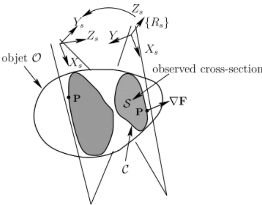
LetO be the object of interest and S the intersection of O
with the US probe plane (see Fig .1 and Fig. 2). The image momentmij of order i + j is defined by:
mij=
Z Z
S
f (x, y) dx dy (1)
where f (x, y) = xiyj and(x, y) represent US image point
coordinates. The objective is to determine the analytical form of the time variationm˙ij of momentmij as function of the
probe velocity v= (v, ω) such that: ˙
mij = Lmij v (2)
where v = (vx, vy, vz) and ω = (ωx, ωy, ωz)
repre-sent respectively the translational and the rotational velocity components and Lmij is the interaction matrix related tomij denoted by:
Lm
ij =
£
mvx mvy mvz mωx mωy mωz ¤ (3)
The time variation of moments as function of the image points velocity is given by [10]:
˙ mij= Z Z S · ∂f ∂x ˙x + ∂f ∂y ˙y + f (x, y) µ ∂ ˙x ∂x + ∂ ˙y ∂y ¶¸ dx dy (4) that can be written:
˙ mij= Z Z S · ∂ ∂x ( ˙x f (x, y)) + ∂
∂y( ˙y f (x, y)) ¸
dx dy
(5) where( ˙x, ˙y) is the velocity of an image point (x, y)
belong-ing to the sectionS. In order to determine the relation giving
˙
mij as function of v, the image point velocity( ˙x, ˙y) needs
to be expressed as function of v, which is the subject of the following part.
A. US image point velocity modeling
Let P be a point of the contourC of the image section S (see Fig. 1 and Fig. 2). The expression of the point P in the US probe plane is:
sP= sR
ooP+ sto (6)
where sP = (x, y, 0) and oP = (ox,oy,oz) are the
coordinates of the point P in the US probe frame {Rs}
Zs Ys Xs Xs Zs {Rs} Ys P P S observed cross-section ∇F C objet O
Fig. 1. Interaction between the 2D ultrasound probe and the concerned object
and in the object frame {Ro} respectively. For the former
it represents the image coordinates of the point P. sRo
is the rotation matrix defining the orientation of the object frame{Ro} with respect to the probe frame {Rs}.stois the
translation defining the origin of{Ro} with respect to {Rs}.
The time variation ofsP according to the relationship (6)
is:
sP˙ = sR˙
ooP+ sRooP˙ + s˙to (7)
We use the classical kinematic relationship that states:
½ sR˙
o = − [ω]× sRo
s˙t
o = −v + [sto]×ω (8)
where[a]× denotes the skew-symmetric matrix associated to the vector a. Thus, replacing (8) in (7), we obtain:
sP˙
= −v + [sP]
×ω +
sR
ooP˙ (9)
The point P results from the intersection of the US probe planar beam with the object. Consequently, in the 3D space, P is a moving point that slides on the object surface with a velocity oP˙ = (o˙x,o˙y,o˙z) in such a way that this
point remains in the US probe beam. Since P remains in the probe plane, its velocity expressed in the probe image frame is sP˙ = ( ˙x, ˙y, 0). Therefore, the relationship (9),
that represents three constraints, has five unknowns (sP and˙
oP). In order to solve this system, two other constraints are˙
needed.
LetOS be the set of the 3D points that lie on the object
surface. Any 3D point P that belongs to OS satisfies an equation of the form F(ox,oy,oz) = 0 that describes the
object surface. The fact that any point ofOS always remains
onOS can be expressed by:
˙
F(ox,oy,oz) = 0 , ∀ P ∈ OS (10)
Assuming that the object is rigid, we obtain:
˙
F(ox,oy,oz) = ∂F
∂oxo˙x +∂∂Foyo˙y + ∂∂Fozo˙z = 0
⇔ o∇F⊤ oP˙ = 0
(11) where o∇F is the gradient of F. It represents the normal vector to the object surface at the point P, as depicted in Fig. 1.
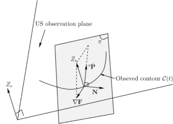
The second constraint concerns the direction of oP. In-˙
deed,∇F defines a plane, denoted by π on Fig. 3, and the constraint (11) states only that the vector oP lies on that˙
plane. We need thus to define in which directionoP lies on˙
π in such a way to match its corresponding pointoP(t + dt)
on the contourC(t + dt). SinceoP(t + dt) is not physically
the same asoP(t), there are many possibilities of matching.
However, since oP is involved by the probe out-of-plane˙
motions, we consider oP in the direction of˙ Zs. Since Zs
does not lie on π, its projection on π is considered as the
direction ofoP. To conclude,˙ oP has to be orthogonal to the˙
vectoroN (see Fig. 3), lying onπ, defined by:
oN= oZ
s×o∇F (12)
such that oZ
s is the expression of Zs in the object frame
{Ro}. It is defined by oZs = sR⊤o sZs. The second
constraint can thus be written:
oN⊤ oP˙ = 0 (13) Y SectionS EdgeC US Image X x P y Fig. 2. US Image
Going back to the relationship (9), it can be written:
sR⊤
o sP˙ = −sR⊤o v + sR⊤o [sP]× ω + oP˙ (14)
Multiplying (14) once byo∇F⊤and then byoN⊤and taking
into account the constraints (11) and (13), yields to:
½o ∇F⊤ sR⊤ o sP˙ = −o∇F⊤ sR⊤o v+o∇F⊤ sR⊤o [sP]×ω oN⊤ sR⊤o sP˙ = −oN⊤ sR⊤o v+oN⊤ sR⊤ o [sP]×ω (15) Since we have: ½ s∇F = sR oo∇F sN = sR ooN= sZs × s∇F (16) The relationships (15) become:
½ s∇F⊤ sP˙ = −s∇F⊤v + s∇F⊤ [sP]
× ω
sN⊤ sP˙ = −sN⊤v + sN⊤ [sP]
× ω
(17) The above system of two scalar equations has two unknowns
˙x and ˙y which yields to the unique following solution: ½ ˙x = −vx− Kxvz− y Kxωx+ x Kxωy+ y ωz ˙y = −vy− Kyvz− y Kyωx+ x Kyωy− x ωz (18) with: ½ Kx = fxfz/¡fx2+ fy2 ¢ Ky = fyfz/¡fx2+ fy2 ¢ (19) such thats∇F = ( fx, fy, fz).
From (18) and (19) we can conclude that the image point velocity depends only of the image point position as for the in-plane motions (vx,vy,ωz) and depends also of the normal
vector to the object surface at that point as for the out-of-plane motions (vz,ωx,ωy). π N Zs US observation plane oP˙ Obseved contour C(t) Zs ∇F
Fig. 3. 3D point velocity vector orientation
B. Image moments time variation modeling
Using the previous modeling of an image point velocity, the image moment time variation,m˙ij can be developed.
The image points for which the velocity was modelled belong to the countour C of S. The image moment variation ˙mij
given by (5) has thus to be expressed as function of these points and their velocities. That is done by formulatingm˙ij
on the contourC thanks to the Green’s theorem:
I C Fxdx + I C Fydy = Z Z S µ ∂Fy ∂x − ∂Fx ∂y ¶ dx dy (20)
Therefore, by taking Fx = − ˙y f(x, y) and Fy = ˙x f (x, y)
in (5),m˙ij is reformulated as: ˙ mij= − I C [ f (x, y) ˙y ] dx + I C [ f (x, y) ˙x ] dy (21)
The image moments can also be expressed on the contourC instead on the image sectionS by using again the Green’s theorem. By settingFx=j+1−1xiy j+1andF y = 0, we have: mij = −1 j + 1 I C xiyj+1dx (22)
and by settingFx= 0 and Fy= i+11 xi+1yj, we also have:
mij = 1 i + 1 I C xi+1yjdy (23)
Replacing now (18) in (21), and then using (22) and (23), we finally obtain the elements of Lmij defined in (3):
mvx = −i mi−1,j mvy = −j mi,j−1 mvz = xmij − ymij mωx = xmi,j+1 − ymi,j+1
mωy = −xmi+1,j + ymi+1,j
mωz = i mi−1,j+1− j mi+1,j−1 (24) where: ½ xm ij = HCxiyjKydx ym ij = HCxiyjKxdy (25) Similarly to the image point velocity, we can note that the terms corresponding to the in-plane motions only depend on the measurements in the image, while the terms correspond-ing to the out-of-plane motions require the knowledge of the normal of the object for each point of the contour. This normal vector could be derived if a pre-operative 3D model of the object was available. That would also necessitates a difficult calibration step to localize the object in the sensor frame. To overcome this limitation, we propose in the next section a method using the successive 2D US images to estimate the normal vector.
III. NORMAL VECTOR ON-LINE ESTIMATION
Let di be the tangent vector to the cross-section image
contour C at point P such that it belongs to that observed image (see Fig. 4). Let dt be an other tangent vector to the
object surface also at P defined such that, expressed in the sensor frame{Rs(t)}, we have:
s ∇F = sdi × sdt (26) Xs Ys Zs D Zi Xi Yi {Ri} ∇F di dt
US observation plane (image) S
P
P0 C(t)
Objet O
Fig. 4. Surface Normals
Since sd
i can directly be measured from the current
image, we just need to estimatesd
t to obtains∇F.
The vectorsdtlies out of the US image plane. Consequently,
it can not be obtained only from the observed US image. We propose in what follows an approach to estimate sdt from
successive images. The principle is to estimate, for each point extracted from the contour C, the 3D straight line that fits a set of successive points extracted from previous successive
images at the same image polar positions (see Fig. 4 and Fig. 5). To illustrate the principle, consider the two cross-section image contours C(t) observed at time t and C(t +
dt) observed at time t + dt after an out-of-plane motion of
the US probe (see Fig. 5). The points P(t) and P(t + dt),
extracted respectively from C(t) and C(t + dt) at the same polar position, lie on the object surface, and thus, a straight
lineD that passes through these points is tangent to the object
surface. The direction ofD is nothing but the tangent vector
dt we want to estimate. In theory, two successive extracted
points are enough to estimate that direction. More will be used in practice to improve the robustness of the estimation. However, since the object surface may be curved, different weights will be associated to the points to take into account this curvature. The complete method is detailed bellow.
The straight line D is defined by its direction id
t =
(dx, dy, dz) and a pointiP0lying on it. They are expressed
in the initial probe frame{Ri}. The point P0is defined such
that each point iP= (ix,iy,iz), expressed in {R
i}, lying
onD satisfies the relation:
¡i
P0−iP¢ × id= 0 (27)
Using a set of points P from the successive US images, the directionid
t can be estimated once the points are expressed
in{Ri} using the robot odometry. From (27) we derive the
following minimal relationship expressing the constraint that the pointiP lies onD:
C(t + dt) D dt C(t) di P(t) P(t + dt) α α
Fig. 5. Soft tissue cross-section 3D evolution
½ ix = η
1iz + η0
iy = τ
1iz + τ0 (28)
where η1 = dx/dz andτ1= dy/dz.η0 andτ0 are function
of iP
0 and id. Thus θ = (η1, τ1, η0, τ0) is the vector
parameters to estimate. The system (28) is written as follows:
Y= Φ⊤θ (29) with Y= (ix,iy) and Φ⊤ = µ i z 0 1 0 0 iz 0 1 ¶ (30)
The goal consists in computing the estimate ˆθ[t] of θ at
least-squares algorithm [11]. It consists in minimizing the following quadratic sum of the estimation errors [12]:
J(ˆθ[t]) = t X
i=t0
λ(i−t0)
θ (Y[i]− Φ⊤[i]θˆ[i])⊤(Y[i]− Φ⊤[i]θˆ[i])
(31) where 0 < λθ ≤ 1 is a weight assigned to the different
estimation errors in order to give more importance to the current measure than to the previous ones. The estimate ˆθ is
given by: ˆ θ[t] = ˆθ[t−1]+ F[t]Φ[t] ³ Y[t]− Φ⊤ [t]θˆ[t−1] ´ (32) where F[t] is a covariance matrix defined by:
F−1
[t] = λθF−1[t−1]+ Φ[t]Φ⊤[t]+ (1 − λθ) β0I4 (33)
where I4 is a4 × 4 identity matrix. The initial parameters
are set to Ft0 = f0I4 with 0 < f0 ≤ 1/β0 and ˆθt0 = θ0. The objective of the stabilization term (1 − λθ) β0I4 is to
prevent the matrix F−1t becoming singular when there is not enough excitation in the input signal Y, which occurs when there is no out-of-plane motion.
We then obtain after normalization id
t =
(ˆη1, ˆτ1, 1)/k(ˆη1, ˆτ1, 1)k and sdt = sRiidt, which
allows estimating∇F using (26). In practice, we use around 400 image points to characterize the contour C.
IV. VISUAL SERVOING
The visual features are selected as combinations of the image moments such that s= s (mij). they are given by:
s= (xg, yg, α,√a, l1) (34)
where xg and yg are the gravity center coordinates of the
cross-sectionS in the image, α its main orientation angle, a its area andl1 its main axis. More precisely, we have:
xg = m10/m00 yg = m01/m00 a = m00 α = 12arctan³ 2 µ11 µ20+µ02 ´ l12 = 2a µ µ02+ µ20+ q (µ20− µ02)2+ 4µ211 ¶ (35) where µij is the central image moment of orderi + j.
The time variation of the visual features vector as function of the probe velocity is written using (24) and (25) as follows: ˙s = Lsv (36) where: Ls= −1 0 xgvz xgωx xgωy yg 0 −1 ygvz ygωx ygωy −xg 0 0 αvz αωx αωy −1 0 0 avz 2√a aωx 2√a aωy 2√a 0 0 0 l1vz l1ωx l1ωy 0 (37) (a) (b) (c) (d) 0 20 40 60 80 100 −1 −0.8 −0.6 −0.4 −0.2 0 0.2 0.4 time (s)
Visual features errors
e 1 e2 e3 e4 e5 (e) 0 20 40 60 80 100 −1 −0.5 0 0.5 1 time (s)
Probe Velocity response (cm/s and rad/s)
v x v y v z ωx ωy ωz (f)
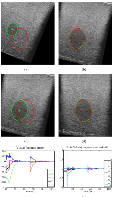
Fig. 6. Results from the ultrasound simulator (the current contour is in green and the desired one in red): (a) Initial and first target image - (b) First target reached after visual servoing - (c) A second target image is sent to the virtual robot - (d) The second target image is reached after visual servoing - (e) Visual error time response - (f) Control velocity applied to the probe
The expressions of some elements involved in (37) are not detailed here for a lack of place. On the other hand, we can notice that the 4th and the 5th component of s (√a and l1) are invariant to the probe in-plane motions (vx,vy, ωz)
and therefore are expected to be well adapted for the out-of-plane motions of the probe (vz, ωx, ωy). On the other
hand, the remaining features xg, yg and α present a good
decoupling for the in-plane motions owing to the triangular part they form. We finally note that the 6th feature remains
to be found to control all the 6 DOFs. A very classical control law is used [8]:
vc= −Lˆ+s K (s − s∗) (38)
where vc is the US probe instantaneous velocity sent to the
Fig. 7. Experimental setup: (left) medical robot equipped with an US probe transducer - (middle) interaction with an US phantom - (right) interaction with a lamb kidney immersed in a water-filled tank
is the desired visual features vector, and ˆL+
s is the pseudo
inverse of the estimated interaction matrix. V. RESULTS
Image processing and control law have been implemented in C++ under Linux operating system. The computations are performed on a PC computer equipped with a 3GHz Dual Core Xeon Intel Processor. The image processing used to extract the US image contour in real-time is described in [13].
In both simulations and experiments, the robotic task consists to reach a first target image and, once this first task has been achieved, a second target image is sent to the visual control system after a certain time span. This allows to validate the ability to re-estimate the normal vector when there has been no out-of-plane motions during that span and also, to analyze the robot behavior during the second task since the estimated normal vector is supposed to have reached the real one. Before launching the servoing to reach the first image target, the robot is moved in open-loop for 10 iterations. This allows providing an initial value to the normal vector. The second task does not need this open-loop motion since an initial value is available from the previous task. At the starting time
t0, the initial parameters vector θ0 is randomly set to (0.2,
0.2, -0.2, -0.2) for all the points of the contour. The initial contour is extracted after a user had roughly indicated it by hand-clicking.
A. Simulation results on a realistic ultrasound volume
We have first used a simulator allowing the interaction of a virtual robotized 2D US probe with a realistic volume of an egg-shaped object. This volume was reconstructed from 100 real B-scan images. This simulator provides the observed US image (see Fig. 6).
The control gain matrix is set to K = 0.7 · diag(1, 1, 1, 1/1.4, 1). The control gain concerning the area
is decreased in order to avoid abrupt robot motion that occur just after launching the servoing. Since at that time the normal vector is not yet correctly estimated. The stabilized least-squares algorithm parameters are set toλθ= 0.8, f0=
1e8, andβ0= 1/(20.f0). The results1are depicted in Fig. 6.
1A short video accompanies the paper
(a) (b) (c) (d) 0 50 100 150 −2 −1 0 1 2 3 time (s)
Visual features errors
e 1 e2 e3 e 4 (e) 0 50 100 150 −0.3 −0.2 −0.1 0 0.1 0.2 0.3 0.4 time (s)
Probe Velocity response (cm/s and rad/s)
v
x vz ωx ωy ωz
(f)
Fig. 8. Experimental results with the ultrasound phantom (the current contour is in green and the desired one in red): (a) Initial and first target image - (b) First target reached after visual servoing - (c) A second target image is sent to the robot - (d) The second target image is reached after visual servoing - (e) Visual error time response (cm, cm, rad, cm)- (f) Control velocity applied to the probe
The visual features errors converge roughly exponentially to zero. This validates the method on realistic US images that are very noisy and thus the robustness to different perturbations like those generated by the contour detection.
B. Experimental results on an ultrasound phantom
We have also tested the method on an US phantom using a 6 DOFs medical robot similar to the Hippocrate system [14] and a 5-2 MHz broadband ultrasound transducer (see Fig 7). In this case, the US transducer is in contact with the phantom, therefore, the probe velocityvy is constrained
by force control to keep the transducer on the phantom surface with a 2N force. In this experiment, we removed
l1 from the visual features vector since we noticed its
coupling with the area a, due probably to the shape of the
observed object in the phantom. The selected visual features are then s = (xg, yg, α,√a). The control gain matrix is
set to K= 0.07 · diag(1, 1, 1, 1/1.4). The stabilized least-squares algorithm parameters have been set to λθ = 0.95,
f0 = 1e8, and β0 = 1/(20.f0). The experimental results1
(a) (b) (c) (d) 0 50 100 150 200 −2 −1 0 1 2 3 time (s)
Visual features errors
e 1 e2 e3 e4 e5 (e) 0 50 100 150 200 −0.1 −0.05 0 0.05 0.1 0.15 0.2 time (s)
Probe Velocity response (cm/s and rad/s)
v
x vy vz ωx ωy ωz
(f)
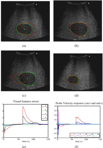
Fig. 9. Experimental results with lamb kidney (the current contour is in green and the desired one in red): (a) Initial and first target image - (b) First target reached after visual servoing - (c) A second target image is sent to the robot (d) The second target image is reached after visual servoing -(e) Visual error time response (cm, cm, rad, cm, cm)- (f) Control velocity applied to the probe
zero and the reached image is the desired one. This validates experimentally the method on a phantom where the images are very noisy and where the experimental conditions are more close to real ones.
C. Ex-vivo experimental results
Finally, we have tested the method in ex-vivo experiments on a motionless real lamb kidney immersed in a water-filled tank (see Fig. 7). The selected visual features are now
s = (xg, yg, α,√a, l1). The control gain matrix is set to
K= 0.07·diag(1, 1, 1, 1/1.6, 1). The stabilized least-squares
algorithm parameters have been set to λθ = 0.8, f0= 1e5,
andβ0= 1/(20.f0). The experimental results1 are depicted
in Fig. 9. Once again, the visual features errors converge to zero and the reached image is the desired one. These results validate the method on motionless real soft tissue.
VI. CONCLUSIONS AND FUTURE WORKS
This paper presented a new model-free visual servoing method based on 2D US images. We addressed shortcomings that were present in our previous work [10]. Moreover, we
have improved and broadened the approach. First, in this work, we have derived the exact analytical form of the interaction matrix related to the image moments. Then, we have endowed the servo system to deal with objects of unknown shape by developing a model-free servoing. For that, the normal vector involved in the interaction matrix has been estimated by a 3D on-line method. Successful results have been obtained in both simulations, experiments on an US phantom, and ex-vivo experiments on a lamb kidney. These results validate the method and its robustness to different perturbations especially those generated by the US image that, inherently, is very noisy. Thanks to the added stabilization term in the on-line estimation, the normal vector identification was achieved even when no out-of-plane motions occurred. This servoing method is generic since it can be applied to different kinds of imaging systems that provide, like US, full information in their observation plane, such as MRI and CT-SCAN. Challenges that remain to be tackled concern the cases of moving and deformable objects.
REFERENCES
[1] P. Abolmaesumi, S. E. Salcudean, W-H Zhu, M. R. Sirouspour, and S P. DiMaio. Image-guided control of a robot for medical ultrasound.
IEEE Trans. on Robotics, vol. 18, no. 1, pp. 11-23, february 2002.
[2] J. Hong, T. Dohi, M. Hashizume, K. Konishi, N. Hata, An ulrasound-driven needle insertion robot for percutaneous cholecystostomy,
Physics in Medecine and Biology, 49(3), pp. 441-445, 2004.
[3] J. Stoll, P. Novotny, R. Howe, P. Dupont, Real-time 3D ultrasound-based servoing for a surgical instrument, in IEEE Int. Conf. on
Robotics and Automation, Orlando, Florida, May 2006.
[4] P.M. Novotny, J.A. Stoll, P. Dupont, R.D. Howe. Real-time visual servoing of a robot using three-dimensional ultrasound, in IEEE Int.
Conf. on Robotics and Automation, pp. 2655-2660, Roma, Italy, May
2007.
[5] M. A. Vitrani, H. Mitterhofer, N Bonnet, G. Morel. Robust ultrasound-based visual servoing for beating heart intracardiac surgery, in IEEE
Int. Conf. on Robotics and Automation, pp. 3021-3027, Roma, Italy,
April 2007.
[6] M. Sauv´ee, P. Poignet, E. Dombre, Ultrasound image-based visual servoing of a surgical instrument through nonlinear model predictive control, International Journal of Robotics Research, vol. 27, no 1, January 2008.
[7] W. Bachta and A. Krupa. Towards ultrasound image-based visual servoing. In Proc. IEEE Int. Conf. on Robotics and Automation, pp. 4112-4117, Orlando, Florida, May 2006.
[8] B. Espiau, F. Chaumette and P. Rives. A new approach to visual servoing in robotics. In IEEE Trans. on Robotics, vol. 8, pp. 313-326, June 1992.
[9] A. Krupa, G. Fichtinger and G. D. Hager. Full motion tracking in ultrasound using image speckle information and visual servoing. In
IEEE Int. Conf. on Robotics and Automation ICRA’07, p. 2458-2464,
Roma, Italy, May 2007.
[10] R. Mebarki, A. Krupa and F. Chaumette. Image moments-based ultra-sound visual servoing. In IEEE Int. Conf. on Robotics and Automation,
ICRA’08, pp. 113-119, Pasadena, CA, USA, May 2008.
[11] G. Kreisselmeier. Stabilized least-squares type adaptive identifiers.In
IEEE Trans. on Automatic Control, vol. 35, n. 3, pp. 306-309, March
1990.
[12] R. Johansson, “System modeling and identification”, Prentice-hall, Englewood Cliffs, 1993.
[13] R. Mebarki, A. Krupa, C. Collewet. Automatic guidance of an ultra-sound probe by visual servoing based on B-mode image moments. In
11th Int. Conf. on Medical Image Computing and Computer Assisted Intervention, MICCAI’08, New York, USA, September, 2008.
[14] F. Pierrot, E. Dombre, E. Degoulange, L. Urbain, P. Caron, S. Boudet, J. Gariepy, and J. Megnien, Hippocrate: A safe robot arm for medical applications with force feedback, Medical Image Analysis (MedIA), vol. 3, no. 3, pp. 285–300, 1999.