HAL Id: hal-00566019
http://hal.univ-smb.fr/hal-00566019
Submitted on 26 May 2021HAL is a multi-disciplinary open access archive for the deposit and dissemination of sci-entific research documents, whether they are pub-lished or not. The documents may come from teaching and research institutions in France or abroad, or from public or private research centers.
L’archive ouverte pluridisciplinaire HAL, est destinée au dépôt et à la diffusion de documents scientifiques de niveau recherche, publiés ou non, émanant des établissements d’enseignement et de recherche français ou étrangers, des laboratoires publics ou privés.
Optimising industrial performance improvement within
a quantitative multi-criteria aggregation framework
Lamia Berrah, Jacky Montmain, Gilles Mauris, Vincent Clivillé
To cite this version:
Lamia Berrah, Jacky Montmain, Gilles Mauris, Vincent Clivillé. Optimising industrial performance improvement within a quantitative multi-criteria aggregation framework. International Journal of Data Analysis Techniques and Strategies, 2011, 3 (1), pp.42-65. �10.1504/IJDATS.2011.038805�. �hal-00566019�
Optimizing industrial performance improvement
within a quantitative multi-criteria aggregation
framework
Abstract: The major industrial control purpose is the reaching of the expected performances. In this sense,
improvement processes are continuously carried out in order to define the right actions with regard to the objectives achievement. Thus, in order to better monitor the performance continuous improvement process, we consider a quantitative model for performance assessment. The industrial performance being multi-criteria, the proposed model is thus based on the one hand, on the Macbeth method to express quantitatively elementary performances from qualitative expert pair-wise comparisons and, on the other hand, on the Choquet integral to express the overall performance according to subordination and transverse interactions between the elementary performances. Then, the main focus concerns the decision-maker’s requirements for optimizing the improvement of the overall performance versus the allocated resources. In this view, we propose useful pieces of information first for diagnosis, then for overall performance improvement optimization versus the costs of elementary performance improvements. Finally, the proposed approach is applied to an industrial case looking for optimizing the improvement of the lean objective satisfaction related to the throughput time of hydraulic component manufacturing.
Keywords:
Industrial performance – improvement process – multi-criteria aggregation – Choquet integral – multi-criteria optimization – Mathematical programming – Decision Support Systems – Industrial case study.
1 Introduction
In industrial engineering, reaching the expected performance level involves generally a continuous improvement process (Deming, 1982). To deal with the current context, new improvement methodologies are gaining wide acceptance, such as Kaizen (Imai, 1986), the Lean Manufacturing (Womack et al., 1990), the six-sigma (Pyzdek, 2001), etc. According to the ISO 9001-2008 standard principles (ISO 9000, 2008), these methodologies generally include the following steps (Berrah et al., 2001; Bradford and Childe, 2001; Womack et al., 1990;
Monden, 1998):
• identifying key areas by defining the objectives, • analyzing the as-is situation by making a diagnosis,
• planning and implementing changes, by choosing the best improvement actions in a given contextwith
regard to the objectives, • monitoring the results,
• and developing a closed-loop control system.
In fact, in this process, the decision-maker must continuously check, diagnose and act. Thus, he needs to get the right information at the right moment, in order to evaluate the success of each step of the considered improvement process before going on to the next one. In our point of view, three aspects of this evaluation to be taken into account are the following:
• the expressions of the achieved performances,
• the diagnosis of what has happened, i.e. to explain the achieved performances,
• the choice of the improvements to be carried out in order to reach the expected performances of the step coming next.
In this sense, decision-making first needs performance expressions which evaluate both the efficacy and the efficiency of the improvement process. While the notion of efficacy is based on the objectives achievement, the efficiency identifies the amount of means used (Neely et al., 1995; Berrah et al., 2008). Secondly, the analysis of the expressed performances should lead, on the one hand, to a diagnosis of what may have happened, and on the other hand, to the definition of “best” improvements.
The problematic of the performance expression is widely considered in literature. According to performance indicators definition, their purpose is to give pieces of information about the objective satisfaction. The current measures are thus linked to the improvement actions to launch (Fortuin, 1988; Bitton, 1990; Berrah et al., 2000). The so-called Performance Measurement Systems (PMS’s) are the instruments commonly used to reach this aim (Bititci, 1995; Bitton, 1990; Globerson, 1985; Ghalayini et al., 1997; Neely et al., 1995). Nevertheless, the performance analysis aspects are generally not formally considered, as decision-makers tend to make decisions in an intuitive manner. In fact, assuming the Taylorian hypothesis (Taylor, 1911; Voss, 2007) that the overall financial performance is nothing more than the sum of independent elementary performances simplifies the decision-making when the improvement deals only with direct manpower productivity. But in the current context of multicriteria performance with different dimensions and transverse interactions, it has become more difficult to identify the performance criteria causing a poor overall performance, or presenting a high-priority need of improvement; moreover this identification must be done very often in a continuous improvement context (at each Deming Wheel’s turn).
The aim of this study is the introduction of the concept of “performance optimization” in an industrial improvement process versus the allocation of resources to the different improvement actions. Indeed, there are many ways to improve the overall performance. Knowing the as-is situation of the system, the different possible improvements depend, on the one hand, on the involved performance criteria, and on the other hand, on the potential actions to be applied to the considered system. Our proposal is to “optimize” the improvement by minimizing the used means for achieving the required overall performance; knowing that this performance is defined by a quantitative aggregation of lower level performances. Note that our approach does not consist in dealing with the efficiency concept through a specific index as in Data Envelopment Analysis approaches (Cooper et al., 2004). The paper focuses more particularly on the definition of useful quantitative synthetic pieces of information first for diagnosis, then for overall improvement optimization versus the costs of elementary performance improvements. This design stage of what an optimized improvement should be is based
on the PMS analysis: material or operational constraints are not introduced. In section 2, the characteristics of the
industrial performance expressions are recalled (Berrah et al., 2004). We precisely consider a data aggregation model that provides a Choquet-integral-based quantitative expression of the overall performance; by considering the elementary performances and the logical qualitative links between them. In section 3, we first explain why and how the diagnosis and optimization key issues can be solved by using an operational research approach. Then the proposed optimization algorithms are exposed. In section 4, this approach is illustrated by means of a practical case study issued from the B Company, which subscribes with a lean improvement approach.
2 The performance expression framework
2.1 Generalities
A PMS can be seen as a multi-criteria instrument, made of a set of performance expressions (also referred to as “metrics” by some authors (Cooke, 2001; Melnyk et al., 2004), i.e. physical measures as well as performance evaluations, to be consistently organized with respect to the objectives of the company. Generally, the considered global objectives are broken down into elementary ones along organizational levels (strategic, tactical or operational). Thus, beyond the objective break-down, one major problem concerns the determination of performance expressions which are useful for the control decision-making (Ducq et al., 2001; Kainuma and Tawara, 2006). Two kinds of performance expressions are involved in a PMS, the elementary ones and the overall ones. The elementary expressions identify the achieved degrees of the different objectives. The overall expressions are the synthesis of the elementary performance expressions. The two main ways to make the synthesis of vectors of elementary performance expressions are the following (Berrah et al., 2004):
• first comparing each component of the vectors and then combining the comparison results, which leads to outranking methods (Mareschal and Mertens, 1991; Babic and Plazibat, 1998) providing a partial order of the vectors; the Pareto front is the most used approach, but Electre and Promethee methods are also encountered (Brans and Mareschal, 2004),
• first aggregating the elementary performance expression of each vector and then comparing the vector aggregation results, which leads to Multi Attribute Utility Theory (MAUT) approaches (Dyer, 2004, Dialoukaki et al., 1992; Rangone, 1996; Bititci et al., 2001; Saaty, 2004; Kulak and Kahraman, 2005; Punniyamoorthy and Murali, 2009; Öztayşi and Uçal, 2009).
In the context of continuous improvement, the step-by-step process requires to be able to observe the performance modifications at the end of each Deming Wheel’s turn. Due to the number of incomparability the outranking methods can lead to, these approaches are not well adapted to see the effects of actions. On the opposite, MAUT aggregation models make the capture of the notion of priorities in the decision-maker’s strategy possible, and simplify the comparison of any two situations described through their elementary
performance expressions. Most of the PMSs echo this point of view (Globerson, 1985, Suwignjo et al., 2000, Berrah et al., 2004) and the weighted average mean (WAM) is generally used to obtain the overall performance. Nevertheless, in the current PMSs, the quantification aspects (related to the parameters of the aggregation operator) are considered as an a posteriori problem, once performance expressions have been selected and defined. This a posteriori definition is no longer adapted to the current context. Indeed, within the current approaches, there is a lack of consistency between the elaboration of the elementary performance expressions and the aggregation expression. In addition, the use of the weighted mean can also be restrictive knowing that the performance criteria are interacting. We have previously seen (Berrah et al., 2004; Globerson, 1985) that more generalized aggregation operators are relevant at the practical point of view, such as the Choquet integral aggregation operator (Grabisch, 1997) which generalizes the weighted mean by taking into account mutual interactions between criteria.
In order to improve the coherence of the information processing involved in PMSs and to provide useful expressions, our proposals lie within the MAUT framework (Figueira et al., 2004), and consist in considering the aggregation problem as a central structuring point. We propose to relate the expressions of the elementary performances to the determination of the aggregation operator in a consistent and meaningful way, in accordance with the measurement theory (Krantz et al., 1971). This leads to consider two aspects:
• the commensurability of the elementary expressions, i.e. two identical performance values along with two different criteria, whatever they are, must correspond to the same satisfaction degree for the decision-maker,
• the significance of the considered aggregation operator, i.e. the comparison (difference, ratio…) of situations based on the aggregated expressions must be the same as the one based directly on the decision-maker’s perception.
In our approach, these aspects are tackled with the MACBETH multi-criteria method (Bana e Costa et al., 2004; Clivillé et al., 2007), which defines quantitative performance expressions and aggregation from qualitative pair-wise comparisons of situations issued from the decision-maker. This is made in the same spirit as the AHP method (Saaty, 2004), by following nevertheless the measurement theory process. Thus the MACBETH method allows the decision-maker to iteratively and coherently define both elementary and aggregated performance expressions for as many situations as considered in the continuous improvement process.
2.2 Backgrounds on the industrial performance expression
2.2.1 The elementary expression
Generally speaking, the transformation of physical measures into performance expressions can be given according to the following mapping (Berrah et al., 2000):
:
P O M× →E
(
o m,)
→P o m(
,)
=pO,M and E are respectively the universes of discourse of the set of objectives o , of the set of measures m and
of the performance expressionp. The key point in differentiating this kind of performance expression from
conventional measurements is in the expression of a satisfaction degree (and not a physical measure), by the comparison of the acquired measures with an objective defined according to the considered control strategy.
Thus, the mapping P denotes a comparison operator such as a distance operator or a similarity operator (Berrah
et al., 2000). This model is closely related to the metrics models (Melnyk et al., 04) which recommend
considering for E a set of meaningful values (monetary value, defect value...). Here, for reasons of coherence of
further information processing, we advocate a specific universe of satisfaction degree forE, i.e. the interval
[0,1] equipped with an adequate structure. 0 means a non-satisfied objective at all and 1 means a fully satisfied objective, and the higher the performance value, the greater the satisfaction.
2.2.2 The aggregated expression
The aggregation of the performance expressions can be expressed as an operation which synthesizes the elementary performance expressions into an overall performance expression. Hence, the performance aggregation can be formalized by the following mapping (Berrah et al., 2004):
1 2
: ... i ... n
Ag E ×E × E × E → E
TheEi ’s are the universes of discourse of the elementary performance expressions
(
p1,p2..., ..., pi pn)
andE is the universe of discourse of the overall performance expressionpAg. As the universesEi ’s and E can be
different, the determination of the aggregation mapping Ag is, generally, not straightforward.
The main aggregation operator is the Weighted Average Mean (WAM) (Globerson, 1985; Suwingjno et al., 2001). This type of compromise operator is well-adapted for independent criteria. Given that this assumption is not always verified, it is possible to deal with the criteria interaction thanks to the family of the Choquet Integral (CI) operators (Grabisch and Roubens, 1996). In our framework, we consider a particular case of Choquet integrals, based on the so-called 2-additive measure: in this simplified model, only interactions by pairs of criteria are considered (Grabisch, 1997). It is possible to consider high order interactions (three or more criteria) but their effects are often neglected by the decision makers while questioned about them.
2.2.3 The 2-additive CI operator
The 2-additive CI involves the 2 following parameters:
1. the weight of each elementary performance expression in relation to all the other contributions to the
overall performance evaluation by the so-called Shapley parameters νi ' s, that satisfy the
condition
∑
ni 1=νi =1, which is a natural condition for the decision-makers,2. the interaction parameters Iijof any pair of performance criteria, that range within [-1,1]:
In the case of the performance expression, the aggregation formula by the 2-additive CI is given by:
n n
Ag i 1 i i i 1 ij i j
1 2
p =
∑
=ν p −∑
= I p −p (1)where
(
p1..., ..., pi pn)
is the vector of elementary expressions with the property: n i j 1 ij 1 0, [1, ], 2 I i n j i ν = ⎛ − ⎞ ≥ ∀ ∈ ≠ ⎜ ⎟ ⎝∑
⎠ (2)This makes the meanings ofν and i Iij clearer, thus providing explanations to the decision-makers on how
the effects coming from the interactions modify a WAM performance.
2.2.4 Example
Let us consider a simple example with 3 criteria to illustrate the preceding concepts in the general context of performance assessment (a continuous improvement case is considered in section 4). In order to compare the overall performance of the different manufacturing lines, let us imagine that we need to aggregate the performances related to the following criteria:
• the takt_time notedp1corresponding to the necessary mean time for each activity of the line,
• the throughput_time1. noted
2
p corresponding to the duration between the product launch and its
delivery,
• the line_flexibility notedp3corresponding to the ratio of daily product manufacturing compared to the
set of products.
For a given line, the current state is described by the following measures:m1=0.12hours m, 82= days m, 0.53= . In
this case, determining directly the manufacturing lines overall performance is a cumbersome task. One manner to proceed is to transform the elementary physical performance measures into satisfaction degrees and to define the relation between the local satisfactions and the overall one by a weighted mean. A solution to make a matching
between the measures and the assigned objectives, (respectively) o1 =0.10, 3o2 = days o, 0.83 = consists in
computing intuitive ratios,as for example:
• 1 1 1 0.12 0.20 0.6 o p m = = = ,
1 Manufacturing throughput_time is defined as the length of time between the release of an order to the factory
• 2 2 2 8 0.29 27.5 o p m = = = , • 3 3 3 0.29 0.58 0.5 m p o = = = .
Besides, the decision-maker has to give both the Shapley parametersν ν ν and the interaction 1, ,2 3
parametersI12,I13,I23, e.g. ν1=0.3,ν2 =0.5,ν3=0.2,I12=0.4,I13= −0.3,I23=0. This means that criteria 2 and 3
are independent and that criteria 1 and 2 have a negative synergy and criteria 1 and 3 have a positive synergy for
the aggregated performance.Hence we can compute:
Ag 1 1 2 2 3 3 0.5 12 1 2 13 1 3 23 2 3 0.36
p =ν p +ν p +ν p − i⎣⎡I ip −p +I ip −p +I ip −p ⎦⎤ = .
But how is the coherence ensured between this ratio procedure and the determination of the aggregation operator coefficients?
2.3 The MACBETH method
2.3.1 The performance aggregation issues
In order to coherently process the aggregation, the elementary performance values must be: • defined on a same commensurate scale on [0,1], generally an interval scale, • coherent with the chosen aggregation operator, generally the weighted mean. As considered in the previous example, this raises two questions:
• how to define the transformation of physical measures into satisfaction degrees? • how to determine the aggregation operator parameters?
The answers are made according to the decision-makers’ knowledge. Thus, to guide the latter in this information processing issue, we propose to use the Macbeth method described hereafter.
2.3.2 The MACBETH principles
The Measuring Attractiveness by a Categorical Based Evaluation TecHnique MACBETH (Bana e Costa et al., 2004) is a MAUT method which requires only qualitative preference judgments about the difference between given situations. MACBETH employs an initial, interactive, questioning procedure which generates a consistent
numerical interval scale from intensities of preference as explained below.In the original MACBETH version a
similar process is appliedto determine criteria weights, but the approach has been extended to determine mutual
interactions between criteria which are further aggregated by a 2-additive CI (Labreuche and Grabisch, 2003; Clivillé et al., 2007). The weight and interaction quantification are deduced from qualitative preferences and
strengths of preference between characteristic performance vectors (0,..,0,1,0,..,0) where for j≠i p, 1i = (which
corresponds to “totally unsatisfying”) and pj = (“not satisfying at all”). In this way, the weights are clearly 0
related to the aggregation formula (and not independently from it), which ensures the coherence of their determination according to the measurement theory (Krantz et al., 1971). The MACBETH procedure consists in four main steps (context definition, elementary performance expression, weights and interactions, overall performance expression) as illustrated hereafter.
2.4 Example of using MACBETH
2.4.1 The context definition step
Let us consider for the overall objective respect_of_takt_time a value of oG= 0.10hour. The considered
contributing criteria are: C1:: components availability (CA), C2:: overall_equipment_efficiency (OEE), C3::
ERP_Data_Relevance (ERPDR). We can consider the set of situations observed at the end of the four last
trimester terms: 1
(
1 1 1)
2(
2 2 2)
3(
3 3 3)
4(
4 4 4)
1 2 3 1 2 3 1 2 3 1 2 3
: , , : , , : , , : , ,
S m m m S m m m S m m m S m m m , where mijare the
corresponding criteria measures. In addition, two situations are declared, as follows:
• the first is referred as good :
(
1 , 2 , 3)
good good good good
S m m m
when corresponding to performance expressions of 1,
• the other one is referred as neutral :
(
1 , 2 , 3)
neutral neutral neutral neutral
S m m m
when corresponding to performance expressions of 0.
2.4.2 The elementary performance expression step
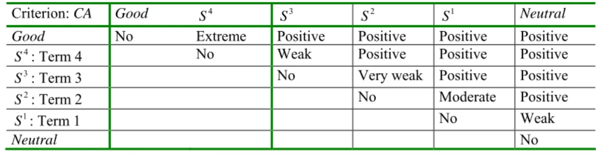
Table 1 gives the collected decision-makers’ preferences and strengths of preferences on a six-level verbal scale (very weak, weak, moderate, positive, very positive, extreme) with regard to the components_availibility
criterion. For example, the decision-maker prefersS2 to S1with a moderate strength, andS3 to S2with a very
weak strength.
Table 1 The preferences and strengths of preference of the decision-maker
Criterion: CA Good S4 S3 S2 S1 Neutral
Good No Extreme Positive Positive Positive Positive
4
S : Term 4 No Weak Positive Positive Positive
3
S : Term 3 No Very weak Positive Positive
2
S : Term 2 No Moderate Positive
1
S : Term 1 No Weak
Neutral No
The quantification of the performance expressions is made by solving the equations system issued from the
expression of all the verbal intensities of preference assimilated to h (with h ranging from 1 very weak= to
6 extreme= ) between k
S and S , written under the form l pk−pl =hα, where α∈[0,1] is introduced to respect the domain bounds (e.g. [0,1]). Thus, the matrix given table 1 leads to the following equation system:
good 4 4 3 3 2 2 1 1 neutral 1 - 6 - 2 - 1 - 3 - - 0 2 p p p p p p p p p p p α α α α α ⎧ = ⎪ = ⎪ ⎪ = ⎨ ⎪ = ⎪ ⎪ = = ⎩
The solution is: 4 0.57 0.43 3 0.35 2 0.14 3
p = p = p = p = .
²Thus, the MACBETH procedure bridges the gap with the current practice that consists in directly determining
an operator of comparison p= f o m( , ) between the objective o and the measure m. Therefore, if the knowledge
of f is available in a consistent way for some criteria, it can directly be included in the procedure, the situation comparisons being superfluous in this case. Note that if we want to obtain the performance expressions for a lot of situations, the procedure becomes a cumbersome task. MACBETH makes a linear interpolation between a limited number of situations. At least, two main situations have to be considered, neutral and good, through the
associated measures neutral, good
m m .
2.4.3 The CI parameters determination step
To determine the n n( +1) / 2 parameters of the 2-additive CI (Shapley indexes υi ' s and interaction
coefficientsI ’s), the decision-maker has to express his preference between two situations ij i
S and j
S . These
situations are evaluated by a 2-additive Cl:
1 1 2 2 1 1 . h h h . . l l l . . i i j i i j n n n n i ij i ij i i j i i j k v p p p I v p p p I α = > = > − = − − + −
∑
∑
∑
∑
(3)where ,v Ii ij=Iji,i=1..n et j≠i and α∈[0,1] are the unknown variables to be determined.
Characteristic situations may be preferred for the pair wise comparison process because they are more easily
interpretable. When situations of type k
(1,..,1, 0,1,..,1)
S = are introduced and compared, the preceding equation
1 1 1 2 2 1 ( ) . 2 n hj lj l h hj lj j i i i h j h i l j l v I v I v v I I kα = ≠ ≠ ≠ ≠ − = − − − =
−
+
∑
∑
∑
∑
∑
(4)And when situations of type k
(0,.., 0,1, 0,.., 0)
S = are compared toSk =(0,.., 0, 0, 0,.., 0), it leads to:
1 , . 0 2 p pj p j p p v I k α ≠ ∀ −
∑
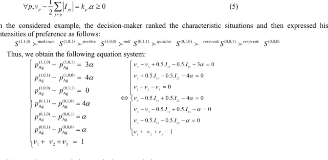
= ≥ (5)In the considered example, the decision-maker ranked the characteristic situations and then expressed his intensities of preference as follows:
(1,1,0) mod (1,0,1) (1,0,0) (0,1,1) (0,1,0) (0,0,1) (0,0,0)
erate positive null spositive veryweak veryweak
S S S S S S S
Thus, we obtain the following equation system:
(1,1,0) (1,0,1) Ag Ag (1,0,1) (1,0,0) Ag Ag (1,0,0) (0,1,1) Ag Ag (0,1,1) (0,1,0) Ag Ag (0,1,0) (0,0,1) Ag Ag (0,0,1) (0,0,0) Ag Ag 1 2 3 3 4 0 4 1 p p p p p p p p p p p p α α α α α ν ν ν ⎧ − = ⎪ − = ⎪ ⎪ − = ⎪ ⎪ − = ⎨ ⎪ − = ⎪ ⎪ − = ⎪ ⎪ + + = ⎩ 2 3 12 13 3 13 23 1 2 3 3 13 23 2 3 12 13 3 13 23 1 2 3 0.5. 0.5. 3 0 0.5. 0.5. 4 0 0 0.5. 0.5. 4 0 0.5. 0.5. 0 0.5. 0.5. 0 = 1 I I I I I I I I I I ν ν α ν α ν ν ν ν α ν ν α ν α ν ν ν − + − − = + − − = − − = − + − = − − + − = − − − = + + ⎧ ⎪ ⎪ ⎪ ⎪ ⇔ ⎨ ⎪ ⎪ ⎪ ⎪ ⎩
In this case, the system admits one single exact solution:
1 0.50 ; 2 0.30; 3 0.20; 12 0.25; 13 0.15; 23 0.15
v = v = v = I = I = I = withα =0.05.
In the general case, when m n> constraints are provided, a linear programming approach can be used to
determine the best set of parameters (Bana e Costa et al., 2004).
2.4.4 The aggregation step
According to the preceding steps, the overall performance expression is:
1 2 3 1 2 1 3 2 3
0.5. 0.3. 0.2. 0.5. 0.25. 0.15. 0.15.
Ag
p = p + p + p − ⎣⎡ p −p + p −p + p −p ⎤⎦
Table 2 summarizes the elementary and aggregated performance expressions for the set of considered situations.
Table 2 Elementary and aggregated performance expressions
Ag p p 1 p 2 p 3 4 S : Term 4 0.50 0.57 0.60 0.37 3 S : Term 3 0.44 0.43 0.55 0.41 2 S : Term 2 0.41 0.35 0.56 0.52 1 S : Term 1 0.26 0.14 0.63 0.50 2.4.5 Summary
By applying the preceding steps, the coherence between the expression of the elementary performances and the determination of the aggregation operator coefficients is ensured. Next, this founded quantitative performance expression model can be used in further issues such as performance improvement.
3. Towards the optimization of the performance improvement
O
nce the considered performances are expressed, in order to achieve the main functions of an improvementprocess, the decision-makers have to periodically consider:
• the diagnosis of what has happened, i.e. to explain the achieved performances,
The purpose of this section is to propose methods to, on the one hand, make the diagnosis of the as-is situation and on the other hand to select the best improvement strategy. Let us recall that in our approach, one “best improvement” is an improvement that joins both efficacy and efficiency, which is thus “optimal” in the sense that it leads to achieve the expected objective by minimizing the resources consumption as exposed in section 1. More precisely, we propose in Sub section 3.1 our diagnosis approach, based on the aggregation performance model seen before (see section 2). Sub section 3.2 summarizes the optimization issues and associated algorithms.
3.1 The as-is situation diagnosis
Let us recall that in our framework the overall objective is broken-down into elementary ones. The questions to be answered by the diagnosis analysis are:
• which elementary performances can roughly explain the current overall performance state?
• which elementary performances could explain in a relative view why a final performance vector
(
1 , 2..., ...,)
F F F F Fi n
p = p p p p has an overall performance superior to the initial performance
vector I
(
1I, 2I..., ..., I I)
i np = p p p p ?
Our idea is to quantify the impact of each elementary performance of p=( ,p1 p2, ,… pn) to the overall
onepoverall =CI p( ), by writing the latter as a sum of contributions:
1 n overall i i p C =
=
∑
where each Cidesignates themarginal contribution of the elementary performance i to the overall performancepoverall. Determining the
elementary performances that contribute best and worst to the achieved overall performance gives the weaknesses and strengths of the current situation. In this view, a linear written per simplex of the 2-additive CI is useful (Akharraz et al., 2002):
( ) ( ) 1 1 ( , , ) n i. i i n CI p p μ p = =
∑
Δ … with ( ) ( ) ( )( ) ( )( ) ( ) ( ) ( ) ( ) 1 1 2 2 i i i j i j j i j i I I σ νμ
> < Δ = +∑
−∑
(6)where (.) is a permutation of indexes such that 0≤ p(1)≤…≤ p( )n ≤1.
Then, the contribution of each elementary performancep to the overall performancei p=CI p( )is simply
.
i i i
C Δμ p. Let us remark that C takes into account both the value of the elementary performance (i p ) and i
the relative importance of criteria (Δμi) in any simplexH(.), whereH(.) { /= p 0≤ p(1)≤…≤ p( )n ≤1}. It means
that the contribution of p to the overall performance may change from a simplex to another one even when there i
is no change regardingp . This effect is caused by the interactions (if the latter are null, the contribution varies i
only with a p change). Thanks to the formi ( ) ( )
1 1 ( , , ) . n i i i n CI p p μ p = =
∑
Δ… , the elementary criteria that have
contributed the most significantly to the value of the overall performance are identified. A convenient explanation approach is to define the level of explanation as the percentage β% of overall performance
contribution and to seek the smallest value n0>0 such that:
0 ( 1) ( 1) ( ) ( ) 1 1 ( ( ), ) . %. . %. ( ) n n n n i n i i i i i Expl CI p β μ p β μ p β Cμ p ≤ − + − + = =
Δ
∑
Δ ≥∑
Δ = , where theΔμ( )i .p( )i ≤ Δμ( 1)i+ .p( 1)i+ valueshave been reordered. Then, Expl CI p( ( ), )β explains CI p up to( ) β%.
The same approach can be applied to relative explanations between a final situation and an initial one by writing: 1 F I n F I p p overall overall i i p p C − = − =
∑
, pF pI iC − being relative contributions.
3.2 The improvement optimization
The notion of optimal improvement is related to the concept of efficient improvement. The search for efficiency is therefore associated to the following questions.
• How to reach the overall objective with a minimal cost attached to the improvement of elementary performances?
Both problems may be formalized into optimization problems in our multi-criteria performance framework. Two main issues are to be distinguished.
• Which elementary performances are to be improved to warranty that a predefined overall objective is reached at the least cost?
• Which elementary performances are to be improved to warranty that a maximal overall objective is reached for a predefined budget?
3.2.1. Reaching a predefine overall objective at the least cost
Let ( ,1 2,..., )
I I I I n
p = p p p be the initial performance profile and pIAg =CI p( I) the associated overall
performance. The problem is to identify the least costly improvement in elementary performance
* * * * 1 2
( , ,..., n )
δ = δ δ δ that achieves an expected overall performance * I
Ag Ag
p > p . Let us denote c pi( , )i δi as the cost
related to a partial improvement from pi topi+δi. For the sake of simplicity, ( , )
I i i i
c p δ is assumed to be a
linear function with respect toδ , i.e.i ( , ) .
I
i i i i i
c p δ =cu δ , with cu being a unit cost. The cost function for an i
overall improvement from ( ) I
Ag
I
p p
CI = toCμ(p+δ), with p=(p1,..,pn) and
δ
=(δ
1,..,
δ
n), can be writtenas2: 1 ( , ) n ( i, ) i i i c pδ c p δ = =
∑
.The search for an efficient improvement may then be formalized into the following optimization problem (P1):
Objective function: min ( , )c p δ δ Constraints: (p ) p* Cμ +δ = ― (behavioral constraint) sup inf , 0 i i i 1 i δ δ δ ∀ ≤ ≤ ≤ ≤ ― (boundary constraints) where inf i
δ
and sup iδ
are threshold parameters derived from the application.3.2.2 Optimal improvement when a budget is predefined
A dual optimization problem (P2) can now be considered for the efficiency characterization: it consists of
computing the maximum expectable improvement for a given additional investment Bδ . (P2) is defined as
follows: Objective function: maxCI(p ) δ +δ Constraints: ( , )p B c
δ
=
δ ― (behavioral constraint) sup inf , 0 1 i i i i δ δ δ ∀ ≤ ≤ ≤ ≤ ― (boundary constraints) 3.2.3 Solving principlesThanks to the piecewise linearity of CI, solving (P1) as a linear programming problem is possible. Indeed,
CIbehaves like a WAM on each simplex (.) { [0,1] / 0 (1) ... ( ) 1}
n
n
H = p∈ ≤ p ≤ ≤ p ≤ . With this property, the initial
problem can be broken down into n! linear programming sub-problems. Nonetheless, this solution used in (Berrah et al., 2008) can only be considered for low n values. Another idea calls for considering the problem as a whole and then introducing complementary linear programming considerations (Dantzig and Thapa, 2003; Sahraoui et al., 2007). For that, let us start with the following statement: Guaranteeing that a potential solution
belongs to a given H(.) implies adding (n−1) constraints to the problem definition:
( ) ( ) ( 1) ( 1)
,
I Ii i i i
p p
i
+δ
+ +δ
+∀
≤
. Next, by noting that all realizable solutions related to a linear programming
problem belong to a convex hull, the associated vertices x exhibit a particular profile due to the three types of
inequalities included in the problem model ( , inf sup 0
i i
i δ δ
∀ = = for the sake of simplicity):
( ) , 0 i i δ ∀ ≤ ( ) ( ) , i 1 i i δ p ∀ ≤ − ( ) ( ) ( 1) ( 1) , i i i i i p +δ p + +δ + ∀ ≤ .
A vertex
x
is thus defined by n equations: (n−1) from the preceding constraints taken to equality togetherwith * ( ) ( ) 1 ( ) .( ) Ag n I I i i i p p CI δ μ δ p =
+ =
∑
Δ + = , whereΔμ( )i ’s are coefficients of the linear expression for CI inthe simplexH(.). The set of constraints is generated for any simplex H(.) and all vertices are computed. The
minimum distance between pI and a vertex yields the solution to the global problem. Let us now remark that
after some rearrangement, a vertex
x
is a vector with 3 distinct coordinate blocks:• unchanged coordinates respecting to the initial vector p (δ( )i = ⇒0 x( )i = p( )i ),
• coordinates equal to 1 (
δ
( )i = −1 p( )i ⇒x( )i =1),• a subset of coordinates with the same value β ( p( )i +δ( )i = p( )j +δ( )j ⇒x( )i =x( )j ).
Linear programming results indicate that I *
p +δ can only assume exceptional values as coordinates, which
means that after the rearrangement, *
p+δ can always be rewritten in the following form, denoted F (Sahraoui et
al., 2007): ( ) ( ) 1,...,1, ,..., , [ ,..., ]T i j p p β β
This proves to be a relevant piece of information for decision-making by generalizing the obvious result obtained with a WAM, i.e. to improve first the satisfaction of the criterion with the highest weight to the maximum.
3.2.4 Sensitivity analysis of the designed improvement
A sensitivity analysis is an important point to check the relevancy or the robustness of the planned improvement. Indeed, it may be of interest to examine how sensitive to perturbations the optimal improvement deduced from
(P1) or (P2) solving is. These perturbations may coincide with unexpected budget variations or the occurrence of
a malfunction that would damage a subset of elementary performances. Sensitivity to budget variations
Solving (P2) for different investment amount δ allocated to performance improvement provides the maximal B
overall performance that can be reached withδ . Thus, when (PB 2) is solved for different investment amounts,
the maximal attainable overall performance can be seen as a function ofδ . The gradient of this function B
provides indications about the impact of the investment increase on the performance increase. Sensitivity to limited elementary performance improvement
Solving (P1) provides an optimal improvement p* =[ ,..,p1* p*n] in the sense of efficiency. The associated cost is
*
C and the improvement vector δ* is such thatp*=pI+δ*. In practice, it may happen that the implementation
of the recommended improvement comes up against difficulties. Some objectives cannot be achieved any longer with the initial planned budget or some constraints cannot be warranted anymore. New decisions are to be made to carry on the improvement project and guarantee a relevant improvement in spite of the malfunctioning occurrence. The optimal improvement must then be revised and adjusted. One issue is to consider the following
optimization problem( 1kI)
P , where Iis the subset of criteria whose optimal performance ∀ ∈i I,δi*cannot be
4 Case study
The case presented here concerns one business unit of the B Company3. First, we describe the industrial system
of the company and the unit considered. Then, we focus on the problem of improvement of the manufacturing
throughput time performance which is tackled by applying the approach proposed in sections 2 and 3.
4.1 The company industrial system
The B Company is one world leader in industrial automation. It designs, produces and delivers pneumatic, hydraulic and mechanic components. The business unit in France designs and produces cylinders and distributors for automation with about 400 people and a turnover of about 60 million €. The company manufactures standardized items (1,300,000 pneumatic distributors, 170,000 pneumatic cylinders, 28,500 hydraulic cylinders) and customized items (32,000 pneumatic distributors, 16,000 pneumatic cylinders and 3900 specific products). The variety of products is very large especially concerning the hydraulic cylinders (a few million possibilities). The manufacturing process is weakly automated, consisting in activities of manufacturing, assembly, finishing, packaging and dispatching. The product is made of about 15 to 25 elementary parts. The manufacturing cycle time is between 2 and 10 days. The production management consists in business planning for product families and Kanban for the component supply.
Since the beginning of the 80’s, the B Company has adopted and progressively generalized continuous improvement approaches. Those ones concern the classical performance criteria such as quality, productivity, safety, and environment and include the logistics, management and lean manufacturing aspects. The “B Company Performance System” is based on the conventional tools of continuous improvement. It focuses on the employee training and the cultural aspects of the lean philosophy. The company wants to improve the lean objectives satisfaction related to the manufacturing throughput time. In this sense, managers would like to have a better explanation of the current as-is situation. They wish to diagnose non-satisfaction reasons and to optimize improvement actions to come. Knowing that the throughput time performance is multicriteria, we will first identify the corresponding performance aggregation model (see section 2). The previous propositions (see section 3) will be thus applied in order to deal with the manager requirements. Note that for the sake of
conciseness, only the hydraulic cylinders HC manufacturing line is considered here (see figure 1).
Figure 1 The HC line.
Cutting
Head & cap
Assembly Tie rod
Piston rod Cylinder
4.2 The throughput time performance aggregation model
4.2.1 The throughput time objective
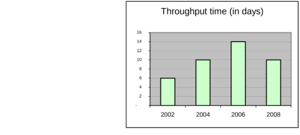
The current state of the HC line does not satisfy its manager. In order to explain this bad lead time of 10 days, two main problems have been identified: the throughput time is too high (see Figure 2)
Figure 2 The manufacturing throughput time evolution
Throughput time (in days)
-2 4 6 8 10 12 14 16 2002 2004 2006 2008
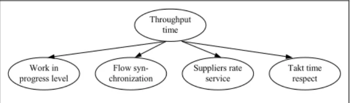
Concerning the throughput time performance, some weaknesses have been identified, leading to breakdown given figure 3.
• The work-in-progress WIP level, • The flow synchronization, • The service rate of the suppliers, • The respect of the takt time.
Figure 3 The throughput time objective breakdown
Throughput time Takt time respect Work in progress level Suppliers rate service Flow syn-chronization
The elementary objectives are quantified by the HC line manager. The description of the current state and the objective quantification are given in table 3.
Table 3 Current state and objective quantification.
Objective label Objective value Figure 4 Current
value
Throughput time 3 days 10 days
WIP level 1 day 5 days
Flow synchronization 0 day 3 days
Suppliers service rate 100% 85.3%
Takt time (respect) 0.100s 0.125s
4.2.2 The elementary performance expression
According to the MACBETH method (see section 2), it is necessary to supply at least 2 measures for each criterion. Table 4 summarizes the collected data.
Table 4 Elementary expression quantification.
Criteria mgood mneutral mintermediary
WIP level 1 day 7 days
Flow synchronization 0 day 5 days Suppliers service rate 100% 65%
Takt time (respect) 0.100s 0.125s 0,110s
It is now possible to associate to each set of measures m m m m1, 2, 3, 4a set of elementary performance expressions
denotedp p1, 2,p p3, 4. A linear interpolation is sufficient except forp4. In this case, the expert has to supply his
strengths of preferences between the 3 retained measures (see section 2). Finally the set of the current elementary performance expressions is given table 5.
Table 5 Elementary performance expressions.
p1 p2 p3 p4
0.33 0.4 0.58 0.00
4.2.3 The overall performance expression
The overall performance expression results from the aggregation of the elementary ones thanks to the CI operator. It is then necessary to determine the operator parameters. Applying the MACBETH questioning procedure to HC line manager has led to the following form:
(1,1,0,1) 1 (1,1,1,0) 0 (0,1,1,1) 5 (1,1,0,0) 0 (0,1,0,1) 1 (0,1,1,0) 3 (0,0,1,1) 1 (0,1,0,0)
Ag Ag Ag Ag Ag Ag Ag Ag
Solving the associated equation system gives the following result:
1 4 / 28 2 11/ 28 3 6 / 28 4 7 / 28 I12 4 / 28 I13 2 / 28 I14 2 / 28 I23 I24 I34 0
ν = ν = ν = ν = = = = = = = .
Note that in the considered case, the whole expertise is provided by one person: the HC line manager. If another person is asked the elementary performances and the CI parameters could be different. Applying the Macbeth procedure to a group of decision makers has not yet been considered.
4.3 The throughput time performance diagnosis
The aim of the HC line manager is to identify the weaknesses and strengths of the situation at each step of the improvement process, namely at the end of the year 2008. The overall performance expression is in the considered case: 1 2 3 4 1 2 1 3 1 4 4 11 6 7 1 4 2 2 2 28 28 28 28 28 28 28 Ag p = p + p + p + p − ⎡⎢ p −p + p −p + p −p ⎤⎥ ⎣ ⎦
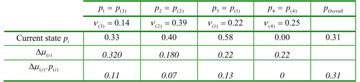
The idea of diagnosis is to determine the elementary performances that contribute best and worst to the achieved overall performance. According to the propositions of section 3, table 6 gives the contribution of each elementary performance to the global one.
Table 6 Elements for diagnosis.
1 (3) p =p p2= p(2) p3= p(1) p4 = p(4) pOverall (3) 0.14 ν = ν(2) =0.39 ν(1) =0.22 ν(4) =0.25 Current statepi 0.33 0.40 0.58 0.00 0.31 ( )i μ Δ 0.320 0.180 0.22 0.22 ( )i.p( )i μ Δ 0.11 0.07 0.13 0 0.31
Intuitively, the contribution of p1=0.33should be weighted by the Shapley coefficient ν1=0.14 that would
correspond to a contribution of about 0.05. In fact, due to the interactions the correct contribution
isΔμ(3).p(3)= Δμ1.p1=0.11. The diagnosis explains what has been done. The next issue is about the
improvement. What must the manager do? Improvingp4, orp2? Compromising elementary performance
improvements? Maximizing the highest weight, the worst elementary performance? Considering associated improvement optimization scenarios provides interesting solutions.
4.4 The throughput time performance improvement optimization
To reachthe objective Throughput_time :: 3 days for the end of 2010, the manager considers to split the action
plan into 4 semesters. The situations at the end of these periods are respectively denoted S2009−1, S2009−2. S2010−1
and S2010−2. The manager would like to obtain the best result as possible for a given investment. According to the
previous considerations, our optimization approach consists in the identification of the efficient improvement. Thus, two strategies are considered:
• a balanced improvement; the investment should be minimal for a constant semester improvement, • a balanced investment; the overall performance should be the best for a constant semester investment. Before going further in the associated computations, let us consider first the improvement cost aspect.
4.4.1 The improvement cost
The HC line manager is asked about the cost of each elementary performance improvement: what is the
necessary budget to improve the elementary expression frompi =0 to pi =1? It is not so easy for him to give
these data. The determination is progressively made by making comparisons between these costs. They are finally given on table 7. For the sake of confidentiality, these values are only indicative.
Table 7 The cost of improvement.
Performance expression label Improvement cost (€)
WIP level 1500
Flow synchronization 4000 Supplier rate service 2000 Takt time (respect) 5000
4.4.2 Balanced optimized improvement
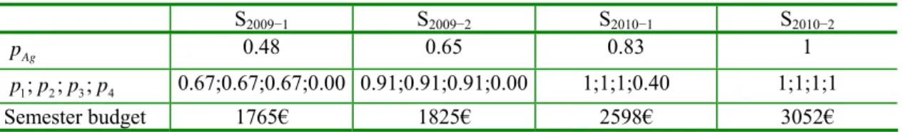
At the end of 2010, situation S2010−2, the overall objective should be reached, i.e. 1pAg = . Moreover the HC line
manager wishes to test the possibility of having a linear improvement during the 4 semesters in order to motivate the employees. The whole improvement being of 0.52, the performance would be improved on 0.17 each period.
For each situation, the minimal investment is computed by solving P1 (table 8).
Table 8 Investment for linear improvement
S2009−1 S2009−2 S2010−1 S2010−2 Ag p 0.48 0.65 0.83 1 1; 2; ;3 4 p p p p 0.67;0.67;0.67;0.00 0.91;0.91;0.91;0.00 1;1;1;0.40 1;1;1;1 Semester budget 1765€ 1825€ 2598€ 3052€
We can notice that the semester budget is increasing. It corresponds to the intuitive idea: the higher the performances, the more costly the improvement. Thus, the HC line manager is now able to define his best intermediary set of performances. He thus defines a step by step efficient improvement.
4.4.3 Balanced optimized investment
In the case of a fixed semester improvement budget, it could be interesting to reach the best overall performance at the end of each semester. Knowing the necessary investment for the total improvement (i.e. 9240€), the HC line manager has a budget of 2310€ for a given semester. Then he has to maximize the overall performance with
this budget. Solving the corresponding optimization problem (P2) leads to the results presented table 9.
Table 9 Investment for constant budget
By applying the frequent encountered practice consisting in improving the lowest performances to a same level, the manager would have considered for the same budget for semester 1 to improve the elementary performances from (0.33; 0.42; 0.58; 0.42) to (0.42; 0.42; 0.58; 0.42) leading thus to the overall
performancepAg = 0.45. Clearly, this practice is not an optimized strategy. Therefore, the possibility of
evaluating the possible improvement in order to maximize the value of pAg for a given budget is of great
interest for the HC line manager.
5 Conclusion and prospects
This paper deals with industrial performance improvement: it more particularly tackles the issue of how to optimize industrial overall performance improvement within a quantitative multi-criteria aggregation framework. This issue is deliberately presented as an information processing problem. In this approach, the major strength is that it warranties the consistency of the whole data process from elementary performances assessment to the design of an optimal overall performance improvement. This consistency mainly relies upon the MAUT framework in which the aggregated performance as overall performance is a central structuring point. This framework provides a powerful representation to capture the managers’ preferences into an analytic form. Then, with this synthetic representation, we can define what an efficacy and efficient improvement should be through muticriteria optimization problems.
Setting up such an approach to improve continuously performance is of great help for decision-makers, however it requires some pretreatments. Indeed, a performance is not a mere measure in our MAUT preference model. The aggregation model requires interpreting the measurements into commensurable utilities-elementary performances- and identifying the aggregation operator parameters. It has been proposed to tackle this point with the MACBETH multi-criteria method, which defines quantitative performance expression and aggregation from qualitative pair-wise comparisons of situations issued from the decision-maker.
Such an indirect identification method is rather well received in industry because it explicitly highlights the role of the experience and the know-how of the company’s experts. In this way, the decision-makers are associated to the design of the decision-making model which appears to be a very significant stake from a user’s
S2009−1 S2009−2 S2010−1 S2010−2 Semester budget 2310€ 2310€ 2310€ 2310€ 1; 2; ;3 4 p p p p 0.74; 0.74; 0.74; 0 1; 1; 1; 0.08 1; 1; 1; 0.54 1; 1; 1; 1 Ag p 0.53 0.74 0.87 1
point of view. Furthermore, the diagnosis functionalities of our decision-making support system provide the decision-makers with explanations which enable them to better understand computations when non-intuitive models as Choquet integrals are required to capture the managers’ strategy. Finally, the proposed quantitative model allows simulating different potential improvement scenarios. These capabilities confer to our information processing chain interesting properties for further man-machine developments. The next step would be the validation in field of the proposed framework.
References
Ahkarraz, A. Montmain, J. and Mauris, G. (2002) Hoschin Kanri, Policy Deployment for Successful TQM, Productivity Press Cambridge, Mass.
Babic, Z. and Plazibat, N. (1998) ‘Ranking of enterprises based on multi-criteria analysis’, International Journal
of Production Economics, Vol. 56-57, pp. 29-35.
Bana e Costa, C. A. De Corte, J-M and Vansnick, J-C (2004) ‘On the mathematical foundations of MACBETH’ in MCDA. Multiple Criteria Decision Analysis, Figueira, J. Greco S. and Ehrgott M., Kluwer Academic Publishers, pp. 409-442.
Berrah, L. Mauris, G. Foulloy, L. and Haurat, A. (2000) ‘Global vision and performance indicators for an industrial improvement approach’ Computers in Industry, Vol. 43, pp. 211-225.
Berrah, L. Clivillé, V. Harzallah, M. Haurat, A. and Vernadat, F. (2001) ‘A cyclic enterprise reengineering method’, International Conference On Engineering Design and Automation (EDA’01), Las Vegas, NV, USA, 6 p., CD-ROM.
Berrah, L. Mauris, G. and Vernadat, F. (2004) ‘Information aggregation in industrial performance measurement: rationales, issues and definitions’, International Journal of Production Research; Vol. 42 (20) pp. 4271-4293.
Berrah, L. Mauris, G. and Montmain, J. (2008) ‘Monitoring the improvement of an overall industrial performance based on a Choquet integral aggregation’, Omega, Vol. 36, (3), pp. 340-351.
Bititci, U.S. (1995) ‘Modelling of performance measurement systems in manufacturing enterprises’
International Journal of Production Economics, Vol. 42, pp. 137-147.
Bititci, U. S. Suwignjo, P. and Carrie A. S., (2001) ‘Strategy management through quantitative modelling of performance measurement systems’, International Journal of Production Economics, Vol. 69, pp. 15-22. Bitton M., (1990, ‘ECOGRAI : Méthode de conception et d’implantation de systèmes de mesure de
performances pour organisations industrielles’, Ph. D. in Control, Université de Bordeaux I, 220 p.
Bradford, J. and Childe S.J. (2001) ‘A non-linear redesign methodology for manufacturing systems in SMEs’,
Proc. of Int. Conf. on Stimulating Manufacturing Excellence in Small and Medium Enterprises (SMESME'01), Aalborg, Denmark, May 14-16, pp. 52-59.
Brans, J. P. and Mareschal, B. (2004) ‘PROMETHEE Methods’, in MCDA. Multiple Criteria Decision Analysis, Figueira, J. Greco S. and Ehrgott M., Kluwer Academic Publishers, pp. 163-189.
Clivillé, V. Berrah, L. and Mauris, G.(2007) ‘Quantitative expression and aggregation of performance measurements based on the MACBETH multi-criteria method’, International Journal of Production
Economics, Vol. 105 (1), pp. 171-189.
Cooke, J.A.(2001) ‘Metrics systems’, Logistics Management and Distribution Report Vol. 40 (10), pp. 45-49. Cooper, W. Seiford, L. and Zhu, J. (2004) Handbook of Data Envelopment Analysis, Springer, 608 p.
Dantzig, G. and Thapa, M. (2003) Linear programming, Springer.
Deming E., 1982, Quality, Productivity and Competitive Position, The MIT Press.
Diakoulaki, D. Mavrotas, G. and Papagyannakis, L. (1992) ‘A multicriteria approach for evaluating the performance of industrial firms’, Omega Vol. 20 (4), pp. 467-474.
Ducq, Y. Vallespir, B. and Doumeingts, G. (2001) ‘Coherence analysis methods for production systems by performance aggregation’, International Journal of Production Economics, Vol. 69 (1), pp. 239-252. Dyer J., (2004) ‘MAUT – Multi Attribute Utility Theory’, in MCDA. Multiple Criteria Decision Analysis,
Figueira, J. Greco S. and Ehrgott M., Kluwer Academic Publishers, pp. 265-295.
Figueira, J. Greco S. and Ehrgott M., (2004) MCDA Multiple Criteria Decision Analysis: State Of The Art
Surveys, (Kluwer Academic Publischers) 1048 p.
Fortuin, L. (1988) ‘Performance indicators - why, where and how’, European Journal of Operational Research; Vol. 34 pp.1-9.
Globerson, S. (1985) ‘Issues in developing a performance criteria system for an organisation’, International
Journal of Production Research, Vol. 23 (4), 639-646.
Ghalayini, A.M. Noble J.S. and Crowe, T.J. (1997) ‘An integrated dynamic performance measurement system for improving manufacturing competitiveness’, International Journal of Operations & Production
Management, Vol. 15, pp. 80-116.
Grabisch, M. and Roubens, M. (1996) ‘The application of fuzzy integrals in multicriteria decision making’,
Grabisch, M. (1997) ‘k-ordered discrete fuzzy measures and their representation’, Fuzzy sets and Systems, Vol. 92, pp. 167-189.
Imai M., (1986), Kaizen : the Key to Japan’s Competitiveness, Mac Graw-Hill Higher Education. ISO 9000-2008, (2008), ‘Quality management systems – Requirements’, Fourth edition, 36 p.
Johnson, D. J. (2003) ‘A framework for reducing manufacturing throughput time’, Journal of Manufacturing
Systems, Vol. 22 (4), pp. 283-298
Kainuma, Y. and Tawara, N. (2006), ‘A multiple attribute utility theory approach to lean and green supply chain management’, International Journal of Production Economics, Vol. 101 (1), pp. 99-108.
Kulak, O. and Kahraman, C. (2005) ‘Multi-attribute comparison of advanced manufacturing systems using fuzzy vs. crisp axiomatic design approach’, International Journal of Production Economics, Vol. 95 (3), pp. 415-424.
Krantz, D.H. et al., (1971) ‘Foundations of measurement, Vol. 1 : Additive and Polynomial Representations’,
Academic Press.
Labreuche C. and Grabisch, M. (2003) ‘The Choquet integral for the aggregation of interval scales in multi-criteria decision making’, Fuzzy Sets and Systems, Vol. 137 (1), pp. 11-26.
Mareschal B., D. Mertens, (1991) ‘Bankadviser, An industrial evaluation system’, European Journal of
Operational research, Vol. 54 (3), pp. 318-324.
Melnyk S., D. Stewart, M. Swin, (2004) ‘Metrics and performance measurement in operations management: dealing with the metrics maze.’, Journal of Operations Management, Vol. 22 (3), pp. 209-218.
Monden, Y. (1998) Toyota Production System: An Integrated Approach to Just-In-Time, Kluwer Academic
Publishers; 3rd Revised edition, 486 p.
Neely, A. Gregory, M. and Platts, K. (1995) ‘Performance measurement system design A literature review and
research agenda’, International Journal of Production Economics, Vol. 48, pp. 23-37.
Öztayşi B. and Uçal, I. (2009) ‘Comparison of MADM Techniques Usage In Performance Measurement’,
Proceedings of 10th Annual International Symposium on the Analytical Hierarchy Process, Pittsburgh, 2009, 11 p.
Punniyamoorthy, M. and Muraly, R. (2009) ‘A framework to arrive at a unique performance measurement score for the balanced scorecard’, International Journal of data Analysis Technqiues and Strategies, Vol. 1 (3), pp. 275-296.
Pyzdek, T., (2001). ‘The six sigma handbook’, Mac Graw-Hill New York.
Rangone, A. (1996) ‘An analytical hierarchy process framework for comparing the overall performance of manufacturing departments’ International Journal of Operations and Production Management, Vol. 13 (8), pp. 104-119.
Roubens, M. (1997) ‘Fuzzy sets and decision analysis’, Fuzzy Sets and Systems, Vol. 90, pp. 199-206.
Sahraoui, S. Montmain, J. Berrah, L. and Mauris, G. (2007) ‘Decision-aiding functionalities for industrial performance improvement’ 4th IFAC Conference on Management and Control of Production and Logistics, Sibiu, Romania, pp. 1-6.
Saaty, T. (2004) ‘The analytic hierarchy and the analytic network processes for the measurement of intangible criteria and for decision making’, in MCDA. Multiple Criteria Decision Analysis, Figueira, J. Greco S. and Ehrgott M., Kluwer Academic Publishers, pp. 345-407.
Suwignjo, P. Bititci, U. S. and Carrie A.S. (2000) ‘Quantitative models for performance measurement system’
International Journal of Production Economics, Vol. 64 (1-3), p. 231-241.
Taylor, F. W. (1911), Shop Management, Harper & Brothers Publishers, New York.
Voss, C. A. (2007), ‘Learning from the first Operations Management textbook’, Journal of Operations
Management, Vol. 25 (2), p. 239-247.
Womack, J.P. Roos, D.T. and Roos, D. (1990) ‘The machine that changed the world’, Free Press, New York, 339 p.