W-NINE: a two-stage emulation platform for mobile and wireless systems

(1)

O

pen

A

rchive

T

oulouse

A

rchive

O

uverte (

OATAO

)

OATAO is an open access repository that collects the work of Toulouse researchers and

makes it freely available over the web where possible.

This is an author-deposited version published in: http://oatao.univ-toulouse.fr/

Eprints ID: 3473

To link to this article: DOI:10.1155/2010/149075

URL: http://dx.doi.org/10.1155/2010/149075

To cite this document:

CONCHON, Emmanuel, PERENNOU, Tanguy, GARCIA, Yohan,

DIAZ, Michel. W-NINE: a two-stage emulation platform for mobile and wireless systems. In

: EURASIP Journal on Wireless Communications and Networking 2010. Special issue :

Simulators and Experimental Testbeds Design and Development for Wireless Networks.

New-York : Hindawi Publishing Corporation, 2010, vol. 2010, Article ID 149075, 20 p.

[Online] Available at

http://www.hindawi.com/journals/wcn/2010/149075.html

. [Accessed

12/04/2010]

Any correspondence concerning this service should be sent to the repository administrator:

(2)

W-NINE: A Two-stage Emulation Platform for Mobile and

Wireless Systems

Emmanuel Conchon

1

Tanguy P´

erennou

2,3

Johan Garcia

4

Michel Diaz

2,3

1

Universit´e de Toulouse, IRIT/IRT-Champollion/ISIS-ISAE, F-81100 Castres, France

2

CNRS ; LAAS ; 7 avenue du colonel Roche, F-31077 Toulouse, France

3

Universit´e de Toulouse ; UPS, INSA, INP, ISAE ; LAAS ; F-31077 Toulouse, France

4

Karlstad University, Sweden

More and more applications and protocols are now running on wireless networks. Testing the implementation of such applications and protocols is a real challenge as the position of the mobile terminals and environmental effects strongly affect the overall performance. Network emulation is often perceived as a good trade-off between experiments on operational wireless networks and discrete-event simulations on Opnet or ns-2. However, ensuring repeatability and realism in network emulation while taking into account mobility in a wireless environment is very difficult. This paper proposes a network emulation platform, called W-NINE, based on off-line computations preceding online pattern-based traffic shaping. The underlying concepts of repeatability, dynamicity, accuracy and realism are defined in the emulation context. Two different simple case studies illustrate the validity of our approach with respect to these concepts.

Keywords: Emulation, Simulation, Wireless Networks

1 Introduction

Testing and evaluating a transport protocol or a distributed application is a challenging task for re-searchers. Indeed, when a new protocol/application is proposed, its behavior has to be compared to the behavior of existing protocols/application. The testing stage is also important for fine tuning the different mechanisms involved in new protocols/applications. In networking and in wireless networking in particular, several difficult points have to be considered to make such an evaluation. In this work, we have chosen to consider three main points: accuracy, dynamicity and repeatability and also a fourth point which can be viewed as a composition of the others: realism.

For this purpose, several solutions can be used. First of them is the use of actual tests, where real applications or communication stacks under test are deployed on the real operational machines. The accuracy of this method is high, but there is a lack of control of environmental parameters. For instance there is no possibility to control the weather conditions when testing a protocol/application in a satellite environment. Furthermore, the experiment cannot be repeated with identical parameters as many times as needed, which is problematic to tune the parameters of the new proposition under test. Such repeatability is highly useful for providing reliable statistical results or to find an optimal operating conditions.

The second solution which is widely used by researchers is simulation, which provides a fully control-lable environment ensuring repeatability. A majoronly need bandwidth delays drawback of simulation is the need for many models: application models, protocol models and traffic models. While some of these may be available, some others can be hard or even impossible to develop (closed source applications). Obtaining the traffic model can also be very difficult especially for multimedia or distributed applications evaluation. Finally, even if the models used for testing are validated, correct behavior of the final imple-mentation has to be verified. For example, it has been shown by [1] that the TCP stack impleimple-mentation in FreeBSD 6 does not behave as expected when losses are inserted at specific position in the real traffic, even though the TCP stack model had been previously validated by simulation.

Network emulation is a compromise between real test and simulation that allows the testing of real applications or transport protocols on an adequate experimentation network while in real time mimicking the behavior of another network. A key interest of network emulation (also called IP-level or level 3

(3)

emulation in this paper) is that only a few parameters need to be manipulated (typically bandwidth, delays and losses). The major challenge is to use accurate models to provide accurate emulation parameters while respecting real time constraints. Some traffic shapers such as Dummynet [2] allow the manipulation of bandwidth, delays and losses. These traffic shapers do not compute network emulation parameters in real time in order to have a very light performance overhead and manage a large amount of packets. Rather, network emulation parameters are provided manually by the end user or automatically by an external source; in the better case, a traffic shaper can be used as basic tools for an emulation platform. Indeed, it must be noted that most of these traffic shapers do not allow the exact repetition of an experiment, especially for the placement of losses.

In this paper, we propose a solution called W-NINE which deals with accuracy by the addition of a simulation stage before emulation time in order to be able to use accurate models to produce the emulation parameters (bandwidth, delays and losses). These simulated parameters will then be used during emulation to evaluate the final protocol implementation under test. Based on accurate models, the proposed simulator generates an emulation scenario that synthesizes all the simulated emulation parameters, providing a dynamic behavior of the network to emulate. Moreover, this emulation scenario can be played several times ensuring part of the repeatability. To further enhance repeatability, a traffic shaper supporting precise loss positioning as well as bit-error insertion can be used to reproduce losses and bit-errors. W-NINE emulation relies on a fully centralized architecture that can be viewed as a “black-box” approach.

The paper is organized as follows. Section 2 provides a brief overview of related work. Section 3 discusses the importance of accuracy, dynamicity, repeatability and realism in network emulation. Sec-tion 4 provides an overview of the proposed architecture and SecSec-tion 5 illustrates the usefulness of this emulation solution with two different case studies. Finally, Section 7 provides the conclusions.

2 Related Work

Emulation systems largely differ depending on the kind of protocol/application to be tested. For example, the properties of the emulation system must differ between the evaluation of a routing protocol and the evaluation of a streaming application. A routing protocol needs a reproduction of the target network topology while most streaming applications only need information about bandwidth, delays or losses and do not care about the network architecture at the link layer. To deal with this specificity, several levels of emulation, depicted on Figure 1 have been defined.

Figure 1: Levels of Emulation

In Level 1 emulation (Physical Level Emulation), only the physical layer is modified in order to be able to mimic the behavior of the target network. For wireless emulation, most physical-level emulators

(4)

are based on a wireless infrastructure and use signal attenuators to reproduce signal conditions that can be observed in the wireless network to emulate. With these attenuators, it is then possible to reproduce the target wireless network topology on an experimentation grid. ORBIT [3] is an emulation platform based on this architecture. The main drawbacks of this solution are that the experiment is not fully controllable. Indeed, due to the use of a real wireless infrastructure, Gamu and al. have shown in [4] that the propagation conditions in the platform can be affected reducing the quality of the provided emulation. To avoid this lack of control caused by interferences, JEmu [5] has proposed the use of a configurable network stack hosting a real implementation of the DSR [6] ad-hoc routing protocol and of the 802.11b MAC layer. JEmu can be seen as a client/server application where the client role is played by a virtual radio layer. This layer is inserted in the configurable protocol stack below the MAC layer and therefore intercepts every packet emitted on the network. These packets are then relayed to a central application that can be viewed as the server. This application then, in real time, simulates node mobility as well as propagation effects to determine if a communication is possible or if collisions might have occurred. If there is no collision, packets are delivered to the destination node; otherwise they can be lost or corrupted according to user configuration. Node mobility can be computed before the experiment so that the amount of computation done in real time is reduced. Nevertheless, the communication support in JEmu is quite simplistic and is only viewed as a communication range. The propagation is limited to the attenuation of the signal based on the distance between the sender and the receiver.

Level 2 emulation (MAC level emulation) is widely used to evaluate real implementations of routing protocols and aims at the simulation in real time of the physical and data link layers. Most of existing solutions are based on a distributed architecture where a virtual MAC layer is embedded on each terminal. This virtual layer needs to provide the same services as a regular data link layer so that the routing protocol under test does not need any modifications. EMWin [7] is a fully distributed wireless emulator focusing on the impact of mobility. For this purpose, an emulated MAC layer has been developed to mimic the medium access CSMA/CA on an ethernet experimentation testbed. Based on neighbor tables, conditions and paths can evolve over time, thus reproducing the dynamic topology of a wireless network. This solution is quite accurate for the mobility purpose but due to the real time MAC emulation and the distributed aspect, repeatability is not fully ensured.

Level 3 emulation (Network Emulation or IP-Level Emulation) allows the evaluation of transport protocols or distributed applications. Typically, only three parameters need to be manipulated to mimic specific network conditions: bandwidth, delays and packet losses. By diminishing the bandwidth, insert-ing delays and packet losses, it is possible to reproduce the same conditions as those encountered at the IP level in the network where the experimentation will take place. Traffic shapers such as Dummynet [2] or NISTNet [8] can be used as basic tools to constrain the experimentation traffic according to user specified rules. These rules are expressed in terms of bandwidth restriction, delays and losses insertions. Seawind [9] is another traffic shaper that has been designed to emulate wireless networks focusing on GPRS networks. It provides a more accurate delay support by specifying allocation, transmission and propagation delays. By using many instances of traffic shapers it is possible to build large emulation testbeds, e.g. Netbed/Emulab [10]. In these large testbeds, various approaches are used to allow the dynamic configuration of a traffic shaper during emulation.

The solution presented in [11] proposed a trace-based emulation system. This emulator mimics a real network on an experimentation one according to previously captured traces. Those traces are then processed to produce an emulation model (i.e. a model made of bandwidth, delays and losses) that will be interpreted by the traffic shaping part of the emulator. This process is known as the “distillation” process. It results in an accurate and repeatable emulation of what happened in the real network. However, capturing traces can be difficult and expensive in time, for instance in large-scale networks. Moreover, traces are a snapshot of specific network conditions at some moment in time. For a user, it is nearly impossible to set up any unforeseen conditions.

Several network emulators such as Mobinet [12] have chosen not to rely on an existing traffic shaper but to develop a specific one from scratch. Mobinet is a wireless extension of ModelNet [13] and is composed of two kind of nodes: the border nodes that will host the virtual nodes where the application and protocols under test are installed and core nodes that will be in charge of the emulation. Mobinet is therefore considered as a centralized emulation solution. To emulate a wireless network, several modules have been implemented: a virtual MAC layer that uses a finite state machine to reproduce the 802.11b medium access mechanism and a virtual routing layer which uses an implementation of the DSR [6] routing protocol. This solution is similar to the one proposed by JEmu but in Mobinet every module can be replaced if necessary. For example, it would be possible to switch from DSR to AODV [14] if an implementation were available. It has also to be noted that the available bandwidth in this emulator is

(5)

very impressive and can support up to 49 concurrent traffics of 49 Mbit/s. Nevertheless, node mobility is not supported and the propagation support is very limited only allowing the computation of propagation effects as a distance function. Moreover, DSR is a very light routing algorithm in term of computation time. Using a more complex routing protocol such as OLSR [15] may have a severe impact on the real time constraints encountered in emulation.

Finally, some level-3 network emulators are based on real-time discrete event simulation such as NSE [16] (the emulation extension of NS-2) or NCTUns [17]. In those solutions, the real traffic is intercepted by the simulator which computes in real time the impact of the wireless network on each packet. The main drawback of this solution is the difficulty to respect real time constraints because the more complex the models are, the more computation time is needed. Even with recent optimizations such as those proposed in [18], NSE is still not scalable and can only support a small set of wireless emulated nodes. For instance in [18], only six wireless nodes, grouped in three pairs, are supported. To further increase performances, the authors investigates the possibility of distributing the real time simulation process but at the time of writing these solutions have not been evaluated.

The remainder of this paper focuses on level 3 emulation.

3 Problem Statement

This section highlights four identified aspects that are challenging for emulators.

3.1 Accuracy

When performing emulation, the accuracy of the emulated conditions should always be considered. The emulated conditions are often meant to reflect actual conditions in a network. The transition from actual conditions to emulated conditions is typically made either by the use of analytical models, simulations or based on traces captured in real networks.

In wireless networks the environment and the behavior of the end user have a strong impact on the observed QoS at the IP level: the current location of the communicating entities and the propagation of the radio signal directly affect delays, losses and the available throughput that IP packets experience. To emulate wireless networks it is necessary to reproduce these effects as accurately as possible. Dealing with movements of terminal nodes may lead to the use of rather complex models to provide a realistic behavior. For example, [19] proposes the use of a database to predict the next position of a terminal according to its previous location, the time and its social relations. People do not act the same way during week end or working days. Their movements have to be affected accordingly.

Similarly, the propagation model often needs to be complex in order to provide results that are sufficiently accurate. If the propagation model is too simple, the behavior is not realistic and this can in turn lead to misinterpretation of experimental results. For instance, relying on a uniform independent packet loss model often leads to false results as shown in [20]. The use of accurate propagation models such as those based on Ray Tracing or on Rayleigh or Ricean random distributions [21] helps to reduce this kind of misinterpretations, but at the expense of large amounts of computation time.

The fact that the most accurate models are typically also the most computationally intensive leads to a trade-off between accuracy and scalability when the models are used in a real-time emulation setting. To avoid this trade-off problem, we developed the use of off-line precomputation of emulation scenarios, which allows the use of accurate but resource demanding analytical and simulation models.

3.2 Dynamicity

There are several sources that contribute to the evolution of network conditions between a pair of nodes in a wireless network: fast and slow fading of the radio signal, node movement and varying cross traffic. The timescale of dynamicity is different among these sources, and so is the nature and complexity of the underlying process. The handling of dynamicity in an emulated environment needs to consider both the need for realistic models and the constraints of emulation.

In the previous section, we have proposed the utilization of an off-line precomputation to use realistic but computationally intensive models. This solution is suitable for the accuracy problem but leads to new challenges on a dynamicity standpoint. First of all is the time granularity challenge. An off-line simulator can produce a dynamic scenario of emulation commands describing the evolution of the wireless network topology. This dynamic scenario can then be played in real time by a traffic shaper on an emulation testbed but the time granularity used between two updates is critical. Indeed, even if accurate models

(6)

have been used for mobility and propagation, updating the emulation conditions only every second will decrease their impact on the realism of the emulation. The used time step results from a compromise: the time step has to be small enough to keep the realism of the used models but also has to be big enough so that the traffic shaper is able to apply emulation commands before the next time step.

The second challenge of dynamicity that has to be faced is directly linked to the emulation purpose. A main advantage of emulation is that no traffic model is needed to provide results and evaluate an application. As a matter of fact, it is not always possible to have a traffic model even for a simulator like NS-2: for instance, it is nearly impossible to model the end user behavior of an interactive application, so the resulting traffic model is hardly ever available. To keep the advantage of not being dependent on a traffic model, it is necessary to avoid the use of a traffic model during the off-line precomputation although, in wireless networks, specific problems such as hidden or exposed terminals are related to the traffic. Dealing with these traffic-based problems has to be done in real time. Two solutions can be considered. First, the simulation process can be done partially in real time as in the EMWin [7] solution. Every node in the experiment can embed a small part of the simulator that will react in real time according to the traffic. The main limitation of this solution is that every node has to be tightly synchronized with the others to ensure the overall consistency of an experiment. Moreover, a dedicated communication protocol has to be set up in order to allow communications among simulator parts. This protocol is used to coordinate the emulation of specific traffic behaviors that involve several nodes simultaneously such as hidden terminals. The second solution to deal with traffic in real-time is to simulate off-line several traffic possibilities and then, on-line, to observe the traffic during the experimentation and to react accordingly. We have chosen this solution because it is less intrusive than the previous one and does not need any time synchronisation between end nodes nor dedicated communication protocol. A more comprehensive description of this solution is provided in section 4.2.

In both cases, the resulting emulation solution has to be over-provisioned to cope with the real time constraints and must use a time step small enough between two emulation conditions updates in order to keep the dynamic aspect and the realism of those conditions.

3.3 Repeatability

The third issue that is highlighted in this paper is repeatability. Repeatability can be considered from multiple viewpoints. On the highest abstraction level repeatability is the ability to identically reproduce any given experiment setup in order to validate the results of an experiment performed earlier. Factors that may cause differences between different runs of an identical experimental setup should be minimized. On a lower abstraction level this translates to the amount of control over the experimental environment that is possible to achieve. From a repeatability standpoint, the maximum possible amount of control of the emulated network is desirable. An analysis of the cause for indeterminism in current network emulators gives at hand that one major contributor is the stochastic insertion of packet losses. When an experimental setup contains a non-congestion-related packet loss element, the random positions of these losses will vary between runs and this variance can have considerable impact on the individual experimental results as is shown in [1]. For instance, if a user wants to compare two error control mechanisms such as FEC or hybrid ARQ, it is necessary to ensure that packet losses will be exactly the same in both cases. If losses do not occur on the same packets, it is hard to examine the behavior of the two error control mechanisms in a fully repeatable fashion and it is also harder to conclude which one has the best performance. Similar arguments hold for bit-errors, for instance in the context of audio/video codec development. To ensure a maximum amount of control over losses and bit errors, deterministic error positioning is needed.

3.4 Realism

Realism depends on the three previous points. For example a high level of realism in a wireless emulation experiment can only be achieved if the emulation is accurate enough to produce highly dynamic conditions and if the emulator is able to reproduce these dynamic conditions in real time. The repeatability also impacts the realism and is highly tied to the design of the emulator. As previously discussed, if an experiment is not fully repeatable then the accuracy is no longer ensured. To sum up, realism is the goal to strive for but not to the detriment of the controllability of the experiment.

(7)

4 W-NINE Architecture

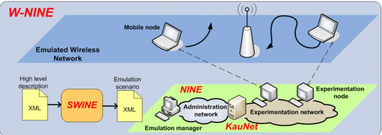
This section describes W-NINE, an emulation platform that addresses the issues of Section 3. As depicted in Figure 2, W-NINE integrates and enhances various existing tools. This integration work was done within the framework of the FP6-IST European Network of Excellence in Wireless Communications (NEWCOM).

Figure 2: W-NINE Architecture.

W-NINE was designed to address the challenges described previously in Section 3. W-NINE is based on an line simulator called SWINE and an emulation platform called NINE. Doing the simulation off-line gives the possibility to use accurate and even realistic models, which are generally time-consuming and cannot be used in real time. To test a protocol or an application, the end user first writes a high-level description of the experiment which is processed by SWINE to produce an emulation scenario that ensures dynamicity. Then the experiment can be repeatedly run in real-time on the NINE platform: the applications and protocols under test are deployed on NINE terminals, while the emulation scenario is played in real-time by the emulation manager. The emulation manager periodically sends emulation commands on the administration network to KauNet [22], a Dummynet extension, used in the central router of NINE. KauNet purpose is to, in real-time, constrain all the IP traffic issued by the terminals on the experimentation network thus mimicking the wireless network where applications and protocols under test will be deployed. KauNet was chosen due to its enhancements in terms of repeatability and accuracy as compared to Dummynet. The behavior of these tools is detailed throughout the remainder of this section.

4.1 SWINE: Simulator for Wireless Network

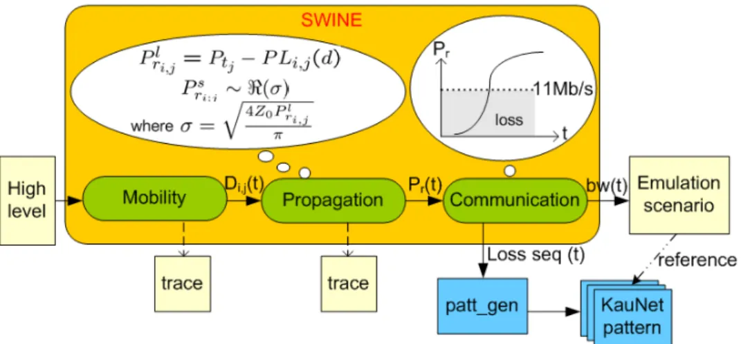
The Simulator for WIreless Network Emulation [23, 24], presented in Figure 3 is an object oriented Java simulator that produces line an emulation scenario based on a high-level description. Doing this off-line gives the possibility to use accurate and/or realistic models that cannot be used in real time. The emulation scenario will be used in the second stage by KauNet.

The emulation scenario and high-level description are both XML files that must be validated against schemas. In this section, the high level description file format and SWINE’s architecture are presented. 4.1.1 High Level Description file

The High Level Description (HLD) file describes the experiment to emulate including obstacles and nodes as well as models used to represent for instance the propagation conditions or the mobility. This file is written in XML due to its simplicity and to the validation possibilities that are available with this formalism. For this validation purpose, the RELAX-NG compact schema (RNC) formalism [25] defined by OASIS has been selected because it is easier to manipulate than regular XSD schemas due to a structure that is close to the Backus-Naur formalism.

As depicted in Figure 4, an emulation experiment starts with the definition of the kind of network that have to be emulated: an 802.11 Ad-Hoc network or a Managed network representing a 802.11 infrastructure network.

(8)

Figure 3: SWINE Architecture

Based on the network type, the world where the experimentation takes place is described. The World is composed of three main elements: concrete elements (such as obstacles, areas and nodes), the time information and the world dimensions. An obstacle is defined by its shape, its position and possibly its signal absorption capability. An Area allows the introduction of a constant PLR in a geographical area and then is defined by its position and its size. Finally, a Node, presented in Figure 5, is mainly composed of the IP information such as its IP address and its gateway but also of its transmission power, its antenna gain, the mobility model that will be used during the simulation to describe its movement and possibly an energy model. Based on the type of network, two kinds of nodes can be considered: mobile nodes and access points which can be viewed as static mobile nodes. This distinction is needed to simulate infrastructure networks. The IP information is provided for the real-time emulation step and is not used directly by SWINE.

The models section describes every model used for the computation of the traffic conditions in the wireless network. These models, such as the propagation model (determines the radio signal level received by a mobile node) or the MAC level model (determines the IP throughput available for the end user), are used by every node in the network. Models used to build cells in an infrastructure network or to find potential hidden terminals situations (see section 4.1.2), are also described in this section. In Figure 6, an example of Pathloss Exponent propagation model [21] description is presented. First, the end user must specify the exponent that will change according to the location of the wireless network and he must also give the reference distance value d0 and possibly the frequency used by the wireless network and the pathloss value at d0.

4.1.2 SWINE’s Architecture

The main difference between SWINE and classical network simulators such as NS-2, Opnet or GloMoSim is that SWINE has been designed for an emulation purpose. SWINE does not evaluate a protocol nor an application but it provides the conditions that the traffic will encounter in the target network. Most of classical network simulators use a layered architecture and simulated packets that go through this layered architecture to provide results. In an emulation approach no traffic model is provided in order to evaluate protocols and applications. This specificity has been kept in SWINE’s design. Therefore, SWINE computes the best conditions that a node might encountered on a communication link, i.e. when it is the only emitting node.

SWINE is a discrete event simulator split in three main steps: Mobility, Propagation and Communi-cation, each step hosting a number of models with an open architecture that allows the easy addition of new and/or more realistic models.

The Mobility step computes all positions of all nodes at every time step of an experiment, using models ranging from the classical random waypoint mobility model to group mobility models such as the Pursue model. All these models can take into account obstacles of the world. Although they are not integrated in SWINE, more complex models such as those which are using social information databases [19] could also be used even though they are time-consuming since there is no time constraint in the off-line preliminary simulation.

(9)

start = Experiment

Experiment = element experiment { element type_of_network {

attribute id {"Ad-Hoc" | "Managed"} }?,

World,

element models { NetModel+ } }

World = element world { element time {

element duration {duration_unit? & real} & element step {duration_unit? & real} } &

element origin {distance_unit? & tuple3d} & element dimensions {distance_unit? & tuple3d} & element obstacles {Obstacle*} &

element areas {Area+}? &

element nodes {Mobile+ & AccessPoint*} } (a) RNC schema <experiment type="Ad-Hoc"> <world> <time> <duration unit="s">179.5</duration> <step unit="s">0.5</step> </time> <origin unit="m"> <x>-2</x> <y>0</y> <z>-2</z> </origin> <dimensions unit="m"> <x>44</x> <y>0</y> <z>44</z> </dimensions> <obstacles> ... </obstacles> <nodes> ... </nodes> </world> <models> ... </models> </experiment>

(b) Associated XML example file

(10)

Mobile = element mobile { attribute id {xsd:ID} &

element models {MobilityModel&EnergyModel?} & element gain {power_unit? & real} &

element tx_power {power_unit? & real} & element ip_address {text} &

element ip_mask {text} & element gateway {text} & element member_of {text} & element mapped_on {text} } (a) RNC schema <mobile id="M1"> <models> ... </models> <gain unit="dB">0</gain> <tx_power unit="dB">-13</tx_power> <ip_address>192.168.106.1</ip_address> <ip_mask>255.255.255.0</ip_mask> <gateway>192.168.106.100</gateway>

<member_of>Emulated WiFi Network</member_of> <mapped_on>wnine1</mapped_on>

</mobile>

Figure 5: An excerpt of the HLD file for nodes

PathLossExponentModel = element stage { attribute id {text} &

attribute class {"swine.models.propagation.PathlossExponentModel"} & element exponent {real} &

element d0 {distance_unit? & real} & element frequency {frequency_unit? & real}? & element pathloss_d0 {power_unit? & real}? }

(a) RNC schema

Figure 6: An excerpt of the HLD file for Pathloss Exponent

The Propagation step uses the positions provided by the mobility step to compute the power of the radio signal received by each node from every other node at every time step of the experiment. Classical propagation models are implemented, including Rayleigh and Rice fading as well as Pathloss Exponent models. Three levels of propagation have been investigated to be as close to reality as possible: large scale effects that are mainly based on the distance between the sender and the receiver; medium scale effects resulting of the signal attenuation caused by obstacles between the sender and the receiver and finally small scale effects which are caused by the multiple paths that the radio signal takes to reach its destination. By combining these three kinds of effects, it is possible to model propagation in a somewhat realistic way. However, the obtained realism cannot be better than the realism of the combined models. As in the mobility step, more complex and time-consuming models such as ray tracing models [26] could be integrated to enhance the realism of the emulation.

The Communication step uses the propagation information to compute the QoS parameters on every link at every time step of the experiment. These QoS parameters form an emulation scenario that can be played by KauNet (see section 4.3.1). The Communication step computes the maximum available bandwidth on a link with a time step of typically 100 ms, as well as KauNet loss patterns with a granularity of 1 ms. Based on the IP information, the Communication step is also in charge of partially dealing with traffic based effects such as hidden or exposed terminals, as further discussed in section 4.2. In future work, the communication step is planned to be extended to more accurately take into account the ad-hoc routing by introducing some delays (caused by route error, route discovery and control messages) on each link according to the routing protocol used.

(11)

On a technical standpoint, SWINE relies on two kinds of objects: domain objects and model objects. Domain objects represent the physical elements of the emulated network (wireless nodes, access points, obstacles. . . ) as well as the wireless links. Model objects represent the equations used to compute the network conditions using domain objects. These two kinds of objects are initialized with the provided high level description file and are then used by the simulation core to fill a link matrix.

The Link Matrix, presented in the UML class diagram in Figure 7, is the key structure in SWINE. In this matrix, the wireless conditions are stored for every unidirectional communications between two nodes at every time step of the experiment. These conditions are composed of the IP Level conditions such as the IP available throughput, delays and losses but also the propagation informations such as the received signal strength on the receiver side, the signal to noise ratio (SNR), the fading, shadowing and path loss effects. These conditions can also take into account any communication conditions such as a potential hidden terminal on the specified communication link.

Figure 7: An excerpt of class diagram focusing on the link matrix.

To fill this link matrix, several models have been implemented. Figure 8 depicts the model hierarchy that has been used to provide conditions to emulate on the emulation platform. From a generic Model class, four kinds of models have been described. The Mobility model, Propagation model and the Com-munication model correspond to the three main steps previously presented and work respectively at the node level, the link level and the link matrix level.

Figure 8: An excerpt of the class diagram focusing on models.

In addition to these three main models a fourth one is provided allowing for example the simultaneous computation of link level informations and of informations that are related to the whole matrix. Hidden terminals [27] are a good example of such a use. In a hidden terminal situation it is necessary to have a look at the full matrix to find the potential three nodes where a hidden terminal can occurs. For example,

(12)

in Figure 9, the node M 2 is in the transmission range of nodes M 1 and M 3. Nodes M 1 and M 3 are out of range of each other, they cannot sense each other’s transmissions. They are said to be mutually hidden. In this case, M 3 can start sending its packets to M 2 while M 2 is still receiving packets from M 1, which may lead to severe interferences and therefore in losses at the IP level on links M 1 → M 2 and M 3 → M 2. Both communication links have then to be updated in the communication matrix so that the hidden terminals situation is reproduced during the emulation stage. This traffic-based behavior emulation is detailed in Section 4.2.

Figure 9: Hidden and exposed terminals situation.

4.1.3 Adding new Models

As previously presented, SWINE is an open architecture that mainly relies on model objects. To insert new models in an easy way, the Java class loader is used, allowing the end user to focus on his own model and not on the simulator itself. Inheriting from a predefined model object class, it is possible to write a new model which will then be usable without any recompilation of the simulator core. As there is a validation of the HLD file provided by the end user before simulation, it is also necessary to extend the provided HLD schema so that the new model can be used.

4.2 Emulation of traffic based behaviors

In wireless networks, instantaneous network traffic has a direct impact on the QoS at the IP level which is far more important than in wired networks. For instance, in Ethernet networks the bandwidth is shared without side effects among nodes which means that if two competing nodes try to send their packets at 10Mb/s and 2Mb/s on a 10Mb/s Ethernet link the first node will only get around 8Mb/s. IEEE 802.11 wireless networks do not behave on the same way. In the 802.11b infrastructure mode, [28] has shown that the maximum available IP data throughput for one node depends on the slowest emitting node. For instance, if a node with a theoretical transmission rate of 11Mb/s (which corresponds to a maximum IP data throughput of 7.74Mb/s) wants to emit at its maximum rate while another node belonging to the same cell emits with a 2Mb/s rate (i.e an IP data throughput of 1.4Mb/s), it will be slowed down until it observes an IP data throughput smaller than 1.4Mb/s. This specificity is directly caused by the CSMA/CA MAC protocol used in 802.11 networks. Other specificities of wireless network are the potential hidden terminals situations previously presented, and exposed terminals. As presented in Figure 9, exposed terminals situation occurs when node M 1 starts a communication with node M 2 while there is a communication between M 3 and M 4. As node M 3 communicates with M 4 and is in range of M 2’s communication, its communication will cause interferences on M 2 leading to packet losses at the IP level.

Due to the architecture of W-NINE, the emulation process of these wireless network behaviors is split in two stages. The SWINE simulation stage computes the different network traffic possibilities and their impact on wireless communications. SWINE looks for every potential traffic occurrences and generates a specific choice in the emulation scenario for each occurrence. According to the 3-steps architecture, the complete network topology and available communication links among nodes at each time step are known after the mobility and the propagation steps. During the communication step, SWINE computes the IP

(13)

parameters that will be reproduced at the emulation stage. First, SWINE’s communication step uses the power received computed by the propagation step to determine the corresponding available IP maximum throughput. Second, SWINE investigates the topology to search all potential traffic-based problems. For example in Ad-Hoc networks, it looks for every group of at least two nodes that can be hidden from each other. If no potential hidden terminal situation occurs, an emulation scenario with a single choice at each time step is produced. But, if there are potential hidden terminals, SWINE produces an emulation scenario with several choices at each time step. The first choice represents the regular situation when no interference occurs, and the other choices represent situations when at least two hidden nodes try to send packets simultaneously to the same node. These other choices are computed according to the user-specified hidden terminals model in the high-level description file (e.g. a 100% packet loss rate). All of these choices provide a multi-branch scenario framework.

During the emulation stage, it is then necessary to observe in real time the network traffic on NINE and to react according to the precomputed choice of the emulation scenario which corresponds to the observed traffic behavior. This mechanism of observation/reaction during an emulation is detailed in Section 4.3.2.

4.3 NINE: Nine is a Network Emulator

NINE is a fully centralized network emulation platform composed of two dedicated networks: the admin-istration network and the experimentation network. This distinction between networks ensures that the administration traffic does not interact with the experimentation traffic and therefore does not impact the experimentation results. On the administration network, the emulation manager is in charge of the configuration of the whole platform whereas the end user nodes are on the experimentation network. The router emulator is on both networks with one Ethernet network interface on the administration network and several Ethernet network interfaces on the experimentation network. The router emulator is the platform core which means that all packets exchanged during an emulation go through it. This central node hosts the KauNet [22] traffic shaper, responsible of the wireless conditions emulation during an experimentation according to emulation manager instructions.

KauNet addresses fine-grained aspects of dynamicity, repeatability and accuracy while the emulation manager addresses the dynamicity issue on a larger time scale as well as a part of repeatability with regards to the emulation scenario. Those different aspects will be discussed later on.

Throughout the remainder of this Section, all components of NINE are presented: KauNet, the traffic observers and the emulation manager.

4.3.1 KauNet

KauNet [22] is an extension of Dummynet, developed by the Karlstad University, that provides the ability to accurately place both packet losses and bit-errors at specific locations in a data transfer to examine transport layer protocol implementations and also application layer effects. These loss positions are gathered in specific pattern files that cover only a small period of the experimentation time. Each pattern can be further reused thus ensuring repeatability for the covered period. The losses and errors can be placed either as a function of the amount of packet transferred (data-driven mode) or as a function of time passing (time-driven mode). These two modes are depicted on Figure 10.

When performing evaluation of implementation correctness it is important to be able to have a large degree of repeatability to recreate experimental runs that produce anomalous effects, so that these can be studied in greater detail and then hopefully corrected. As mentioned earlier, the placement of packet losses can have a large impact on the behavior of both transport layer protocols and also application behavior. While the basic protocol mechanisms can be studied by injecting losses in a controlled way using a simulator, this does not help to verify the behavior of actual implementations. KauNet was developed to provide a tight control over the accurate placement of losses during a live experiment involving real implementations and real traffic. More technical details can be found in [22].

4.3.2 Traffic observers

The traffic observer (TO) module has been developed to observe in real time the network traffic crossing the NINE experimentation network. The TO is a C++ module hosted on the router-emulator, using a CORBA connection to interact with the emulation manager during the emulation stage. A traffic observer takes no decision, its purpose is to inform the emulation manager when a specific traffic condition occurs

(14)

(a) Data driven mode

(b) Time driven mode Figure 10: KauNet loss insertion

on a communication link. Note that if several traffic conditions have to be investigated (e.g. several hidden terminals situations), several TOs are needed.

At the beginning of the experiment, TOs are configured by the emulation manager to observe specific nodes. Then, using feedback mechanisms, a TO sends information relative to the observed traffic to the emulation manager which selects the corresponding precomputed choice of the multi-branch emulation scenario at the current time step. For example, if a TO has a couple of nodes under observation in order to determine if they are hidden from each other at time t, it observes the traffic emitted by both nodes and informs the emulation manager when both traffic flows reach the router-emulator during the same time step. The size of this time step and the sets of nodes that must be observed are set by the emulation manager at the beginning of the experiment.

The decision process is centralized in the emulation manager because it is the only node of the ad-ministration network that has a complete view of the experiment and of different scenarios. For an administration purpose, this centralized solution is far simpler than distributing the decision process between the emulation manager and TOs. With this centralized solution, KauNet receives update com-mands only from the emulation manager whereas in a distributed solution a priority scheme between the emulation manager and traffic observers should be set up. The overall deployment process is presented in Figure 11.

(15)

A limitation of this solution is that the detection of a situation by traffic observers and the reaction of the emulation manager are not simultaneous. The emulation manager sends KauNet update commands according to the time granularity of the precomputed emulation scenario. That means that in the worst case, KauNet reacts a full time step after the traffic observers’ detection.

4.3.3 Emulation Manager

The emulation manager is a stand-alone Java application in charge of the emulator configuration and of playing the precomputed emulation scenario. The scenario is a natural way to repeat an experiment as often as needed. During an experiment, the emulation manager periodically sends update commands to the emulator in order to make the emulated conditions evolve dynamically.

During NINE configuration, the emulation manager builds every communication link that might be used during the experiment. Communication links are represented by Dummynet pipes in the emulator. According to the precomputed multi-branch emulation scenario, the update commands are periodically sent during an experiment by the emulation manager through the administration network to KauNet. These update commands lead to the evolution of communication links’ characteristics in terms of band-width, delays and losses over the whole experiment duration. Between two update commands, KauNet is in charge of reproducing the simulated wireless conditions, on a finer time scale which improves accuracy and dynamicity.

5 Use Cases

In this section, we highlight with two examples the effectiveness of the methodology and discuss about potential enhancements. First, a simple example presents the KauNet loss pattern generation with SWINE; in this example we compare the emulation result with SWINE simulation results and with the measurements made during a similar real experiment. A second example presents the use of traffic observers to deal in real time with traffic-based behaviors during emulation.

5.1 A Simple Indoor Wireless Communications Experiment

5.1.1 Description of the experiment

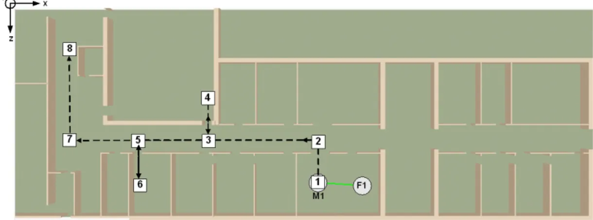
Figure 12: A dynamic experiment.

In the experiment illustrated by Figure 12, a mobile user receives a multicast UDP data flow while going through different areas of our offices in Toulouse. At the beginning of the experiment, the user starts close to a stationary sender (F1). Then, he follows the path 1 → 2 → 3 → 4 → 3 → 5 → 6 → 5 → 7 → 8 with a speed of 1 m/s. At t = 0 the user starts its movement from his office at position (1), then he enters the corridor (2) and turns to the lecture room (3) which he reaches at t = 21.3 (4); he leaves the lecture room and reaches the secretary’s office (6) at t = 35.8; finally he leaves the secretary’s office to go to the exit (8).

While the user is moving, the sender generates a multicast UDP flow with 1472-byte long packets in CBR (constant bit rate) mode. The CBR throughput is 4.19 Mb/s which is the theoretical maximum

(16)

throughput for a physical transmission rate of 5.5 Mb/s in multicast mode. This 4.19 Mb/s throughput was used so that packet losses can only result from the emulation of wireless losses and not from buffer overflow on the emulation node. Since multicast is used, the link layer will not perform retransmissions. 5.1.2 Live Test Measures

A live test measurement campaign has been performed in our labs, trying to reproduce as close as possible the previous parameters, i.e. the mobile trajectory and CBR traffic. Results are depicted on Figure 13 with a granularity of 500ms. 0 20 40 60 80 100 0 5 10 15 20 25 30 35 40 45 50 55 60 0 5 10 15 20 25 30 35 40 21.3 35.8 PLR (%) Distance (m) Time (s) Waypoint passing time (s)

Measured PLR on F1->M1 F1->M1 distance

Figure 13: Live test PLR measure.

It can be observed that the PLR increases as the distance increases. This curve will be used as a basis of comparison to evaluate the emulation results provided by W-NINE.

5.1.3 Modeling packet losses on a Wireless Link

A key point in wireless networks emulation is the modeling of the environment. We use a propagation model to compute the evolution of the PLR over time. A number of propagation models that match many different environments and radio technologies [21] have been developed. We use a combination of a pathloss exponent model and a Rayleigh fading model to provide a reasonably realistic model for an indoor environment (i.e. such a model accounts for both large-scale and small-scale variations of the radio signal). The following experiment shows that a combination of mobility and propagation models can be used to provide more realism when emulating a mobile wireless LAN. Moderately complex models are used here, but much more complex ones could be used to further enhance realism without compromising real-time constraints, since computations based on these models are entirely done off-line before emulation time.

The radio signal propagation conditions are described by a combination of pathloss exponent, shadow-ing and Rayleigh fadshadow-ing models. The parameters of the pathloss exponent model are n = 3.11, d0= 1 m and P L(d0) = 37.28 dB. The shadowing model is configured with standard deviation σ = 4.25dB. Those parameters were estimated using linear regression on the measures of received signal strength (RSS) presented in Section 5.1.2.

5.1.4 Simulation results

During the simulation stage, SWINE computes the positions of M 1 as well as the propagation infor-mations. These propagation informations are used to generate small-sized 100 ms-long KauNet packet loss patterns with a 1 ms granularity. As the experiment is 60 s long, 600 KauNet packet loss patterns

(17)

0 20 40 60 80 100 0 5 10 15 20 25 30 35 40 45 50 55 60 0 5 10 15 20 25 30 35 40 21.3 35.8 PLR (%) Distance (m) Time (s) Waypoint passing time (s)

SWINE Simulated PLR F1->M1 Distance

Figure 14: Simulated losses with SWINE.

have been generated. At emulation time, the emulation manager updates the pattern to be played every 100 ms. All patterns are used in a data driven way so that the same packet is lost from one run to another.

Figure 14 shows the evolution of the PLR during the experiment. The PLR curve is averaged with a 500 ms interval to improve readability. It can be observed that the losses increase as the distance increase. The small variations that can be observed on the PLR curve are due to the fading model effects.

The results are obviously very different between simulation (and therefore emulation) and real mea-surements. We nevertheless consider that these differences should not be considered as a problem: they simply show that the models used during the simulation stage were not realistic enough. The platform proposed here allows to reproduce with a good fidelity the output of the simulation stage. Realistic emulation therefore depends on the availability of realistic propagation and mobility models as well as MAC and PHY layer models. This topic is extensively discussed in [?].

In the example developed in this section, the propagation model does not take into account the building materials, nor even the number of walls between the sender and the receiver. With such a model, the variations of the simulated signal strength are pessimistic when there are no walls and optimistic otherwise. The litterature proposes more sophisticated models, like the Motley-Keenan model or the COST 231 Multi-Wall Model which will be integrated to the SWINE simulator in future work. On another level, the mobility model used at simulation time supposes a constant speed. The real trajectory of the walking operator during the live tests was not captured, because we did not have accurate indoors positioning tools, which also introduces differences in the results.

5.1.5 Emulation results

During the emulation stage, the MGEN [29] traffic generator is used to send the desired CBR traffic (4.19 Mb/s) and to collect the packets received by the user. The TRPR tool is then used to generate the PLR curve based on MGEN traces with a 500 ms granularity.

As presented in Figure 15, losses increase with the distance as expected. The PLR observed during emulation is quite similar to the one observed during simulation, but shows stronger variations. These variations are due to the packetization by MGEN, which cannot guarantee that the exact same number of packets is sent during each 500 ms slot. In these conditions, we consider that the measured PLR is consistent with the simulated one. The performance of KauNet on its own is further examined in Section 6.

(18)

0 20 40 60 80 100 0 5 10 15 20 25 30 35 40 45 50 55 60 0 5 10 15 20 25 30 35 40 21.3 35.8 PLR (%) Distance (m) Time (s) Waypoint passing time (s)

Measured PLR on F1->M1 F1->M1 distance

Figure 15: Measured losses on NINE.

5.2 Example of traffic-based emulation

In this use case, we will highlight the usefulness of traffic observers to detect a hidden terminals situ-ation and present the selection process that is made by the emulsitu-ation manager in order to apply the corresponding emulation command.

5.2.1 A classical hidden terminals situation

In this example, a mobile node M 1 and two stationary nodes F 1 and F 2 are used. As shown in Figure 16, M 1 goes through the corridor starting from position 1, located close to F 1 and stops at position 3 located at the end of the corridors with a speed of 1.5 m/s. The chosen mobility model is simple in order to make the emulation results more readable. F 2 is located between waypoints 2 and 3.

Figure 16: Example of hidden terminal experiment.

In this topology, nodes F 1 and F 2 are not within range of each other and they are not aware of a potential transmission from the other: this is a typical case where a hidden terminals situation can occur. The propagation of the signal has also to be considered in order to have a reasonably realistic experiment. To deal with propagation a Rayleigh fading model and a Pathloss Exponent model have been used. The parameters of the pathloss exponent model are n = 5.68, d0 = 1 m and P L(d0) = 19.97 dB. They are slightly different from the previous experiment because there is no shadowing model explicitly used in

(19)

this experiment. As in the previous experiment, a multicast UDP flow with 1472-byte long packets in CBR (constant bit rate) mode is used.

The hidden terminals model used during simulation to generate the different choices in the emulation scenario is an ON/OFF model. With this model, when two concurrent signals are received at the same time by the same node, all packets are lost for a time slot duration (100 ms).

5.2.2 Simulation results

The simulation stage generates several choices in the emulation scenario for every potential hidden ter-minals situation. The generated scenario, presented in Figure 17, details these different choices. The emulation manager is aware that several emulation commands might be sent at a specific moment for a specific communication link and therefore that it has to check for traffic information in order to choose the correct one. A TO called F 1 − M 1 − F 2 is then configured to observe the traffic transmitted by nodes F 1 and F 2 in order to detect their communication to M 1.

<link_update hidden="0" hidden_id="F1-M1-F2"> <on_link id="F1 to M1" /> <bandwidth unit="b/s">6870000.0</bandwidth> <plr unit="percent">0.0</plr> <delay>0</delay> <queue_size>8</queue_size> </link_update>

<link_update hidden="1" hidden_id="F1-M1-F2">

<on_link id="F1 to M1" /> <bandwidth unit="b/s">6870000.0</bandwidth> <plr unit="percent">100.0</plr> <delay>0</delay> <queue_size>8</queue_size> </link_update> ... </date>

Figure 17: Excerpt of the emulation scenario: two choices for hidden/not hidden traffic conditions. As presented in section 4.2, SWINE checks the wireless network topology at every time step of the experiment in order to find a topology with potential hidden terminals and generates two choices when an occurrence of hidden terminals is possible: at t = 8400 ms if the TO detects only one sender, the hidden terminals situation does not happen and so the first choice is applied (PLR=0%); if the TO detects several senders at the same time then the second choice is applied and all packets are lost (PLR=100%). More precisely, this last choice means that if nodes F 1 and F 2 simultaneously send packets to the same node M 1, all of these packets are lost.

Figure 18 (a) and (b) present the simulation results in term of IP throughput for communications F 1 → M 1 and F 2 → M 1 when only one sender is active. For F 1 → M 1, the maximum IP throughput gradually decreases until the communication is lost at t = 26.2 s. The communication F 2 → M 1 is possible only after t = 6.6 s and the observed IP throughput increases progressively as the node M 1 is coming closer to F 2.

Figure 18 (c) and (d) present the other possible conditions when both senders are active at the same time. We can see that the node M 1 no longer receives new packets between t = 15 s and t = 20 s. More generally, both communications are highly degraded with regards to the previous possible conditions. 5.2.3 Emulation results

To highlight the emulation results, the communications from the senders are started at different moments. Communication F 1 → M 1 starts at the beginning of the experiment and stops at t = 20 s. The other communication F 2 → M 1 begins at t = 5 s and stops at the end of the experiment. With this pattern, the hidden terminals situations can be encountered only after t = 5 s and so the first choice (no hidden terminals) of the scenario is applied at each time step before this time. After 5 s, the TO running on the emulator detects concurrent traffics from F 1 and F 2 on the experimentation network. It informs the emulation manager of the detected hidden terminal situation. The emulation manager then applies the 100% PLR choice at each time step. At t = 20 s, as transmission F 1 → M 1 stops, there are no more hidden terminals so the first choice of the scenario is applied to the transmission F 2 → M 1 at each time step.

(20)

0 1000 2000 3000 4000 5000 6000 7000 0 5 10 15 20 25 30 35 40 Throughput (Kb/s) Time (s) F1 -> M1 communication

(a) F1 to M1 throughput without hidden terminals

(b) F2 to M1 throughput without hidden terminals

(c) F1 to M1 throughput with hidden terminals

(d) F2 to M1 throughput with hidden terminals Figure 18: Two simulated possibilities of a hidden terminal scenario.

As presented in Figure 19, the obtained results are consistent with our expectations. Until t = 5 s, the F 1 → M 1 communication has no perturbation and the measured throughput is the same as the simulated one. After t = 5 s, the decrease of the IP throughput is considerably larger than for the simulation without hidden terminal. The hidden terminals situation has been detected by the TO and the emulation manager has applied the 100 % loss choice between t = 5 s and t = 20 s. After t = 20 s, the IP throughput variations are smaller and are consistent with the simulation of the communication F 2 → M 1 without hidden terminals. The TO has detected that the communication F 1 → M 1 is over and that the node F 2 is the only remaining sender. With this detection, the emulation manager has switched from a hidden terminals situation to the regular one where there is no interference.

6 Performance Evaluation

In this Section, we measure how accurately KauNet loses packets and we evaluate its performance from the CPU usage and memory footprint standpoints.

6.1 Setup

The evaluation of accuracy, CPU usage and memory footprint were performed using the same setup. A sender, a receiver and a KauNet 1.0.0 box were connected to a gigabit Ethernet switch. The three machines used were simple IBM R50e laptops with 768 MB memory, 1.4 GHz processor and a gigabit Ethernet interface. The sender and receiver run the Linux Ubuntu 8.04 OS, while the KauNet box runs a FreeBSD 7 OS compiled with KauNet support. The unique gigabit Ethernet interface of the KauNet box is configured with two virtual interfaces, one connected to the sender and the other one to the receiver.

(21)

(a) F1 to M1 measured throughput

0 1000 2000 3000 4000 5000 6000 7000 0 5 10 15 20 25 30 35 40 Throughput (Kb/s) Time (s) F2 -> M1 communication (b) F2 to M1 measured throughput Figure 19: Emulation results with a hidden terminal occurrence.

6.2 Accuracy of Packet Losses in Time-Driven Mode

To measure how accurately KauNet loses packets in the time-driven mode, we have generated a number of loss patterns and used the iperf [?] traffic generator to measure how many packets were effectively lost by KauNet. The loss patterns were manually generated with different packet loss rates: 1, 5, 10, 25, 50, 75 and 99 %, and with different durations: 100, 500 and 5000 ms. For each of these 24 packet loss patterns, iperf was used to transmit different constant bitrate (CBR) traffics from the sender to the receiver through the KauNet box, loaded with the pattern under test in time-driven mode. The tested bitrates were 100 kbps, 1 Mbps and 10 Mbps. For each bitrate, different packet sizes were used: 64, 512, 1024 and 1472-byte long UDP PDUs. Once the bitrate and the packet size were fixed, the sending time is computed so that a significant number of packets goes through KauNet. This significant number is set with a rule of thumb stating that 100 packets are needed to test 100 % of the 1-ms timeslots for packet loss or no loss, and that this must be done several times (here 30 times) to gain statistical significance. Hence the sending time is set so that at least 3000 packets are sent and there is traffic during the whole longest 5-second pattern.

To sum up, there are 24 patterns to test, each with 12 different iperf CBR setups. For each pattern generated with PLRg, iperf provides the observed packet loss rate PLRo and we measure the absolute error accuracy Eabs = PLR_g_{− PLR}_o. A negative error indicates that there were more losses than expected.

Figure 20 displays all the absolute accuracy error Eabs results. Each subplot has fixed iperf traffic conditions and contains three curves, one for each pattern duration; each curve shows the absolute error Eabs observed as a function of the corresponding PLRg.

The results are very good since in more than 90 % of the cases the absolute error is less than 5 %. The only case where the relative error gets very high is for the 10 Mbps traffic made of tiny 64-byte packets: in that case, instead of e.g. a 1 % PLR we observe a 43 % PLR, i.e. 43 times more or a 4300 % relative error. Under these traffic conditions however, even without any KauNet pattern loaded, iperf observes an erroneous 6 % PLR. This is due to the hardware used, which is not powerful enough to correctly manage the 13 packets seen during each millisecond. Future works includes running the same tests on a more powerful KauNet box.

To get a more precise idea of the performance of KauNet we also measured the relative accuracy error Erel = (PLR_g_{− PLR}_o)/PLR_g. Figure 21 displays all the corresponding results.

These results are good too: in most cases, the curves are close to 0, which means a negligible relative error. For small values of PLRg, relative errors of 5 % or less are often observed: these error are still acceptable. For instance a 2 % relative error on a 5 % PLR gives a 5.1 % observed PLR. These small differences are due to the fact that a packet may not exactly fall into the appropriate loss timeslot. More importantly, larger errors of typically 40 % are often observed for PLRg = 1 %. This is currently under investigation.

(22)

Figure 20: Absolute packet loss accuracy error.

6.3 CPU Usage and Memory Footprint

Running all the above tests takes approximatively 6 hours, taking into account systematic resynchroni-sation of the 3 machines, pattern loading and processes starts/stops. During these 6 hours, we measured the CPU and memory usage on the KauNet box using the vmstat system command. The results are illustrated by Fig. 22. Most of the time, the CPU load is lower than 5 %. Periodic peaks observed cor-respond to independent periodic tasks that we did not remove. The final CPU load peak corcor-responds to the experiments where iperf generates a lot of packets and corresponds to the anomalies described above. Here again, turning to a more powerful KauNet machine can improve the results.

Fig. 22 also shows that the amount of free memory is rather stable and that the repeated loading of patterns during the execution of the tests does not cause any large fluctuations in the amount of allocated memory.

7 Conclusion

In this paper we have presented an emulation platform called W-NINE that improves accuracy, dynamicity and repeatability of the emulated network conditions of a given experiment in order to increase the realism of the experiment. For this purpose, W-NINE is split in two stages. First is the simulation stage based on SWINE, a wireless discrete event simulator which does not need a traffic model to provide results contrary to classical simulators like NS-2. The main purpose of SWINE is not to provide results directly usable by the experimenter but to generate an emulation scenario describing the evolution of conditions (expressed in terms of bandwidth, delays and losses) in the network to emulate. After the simulation stage is the emulation stage relying on NINE, a fully centralized emulation platform composed of three elements: the emulation manager in charge of the management of the experiment; the KauNet traffic shaper in charge of reproducing the emulated conditions according to emulation commands sent by the emulation manager; and finally traffic observers that check the traffic going through the central node in order to provide feedback to the emulation manager when needed. This traffic observation has been made in order to detect any traffic-related conditions such as hidden terminals for ad-hoc networks.

The usability of W-NINE has then been highlighted with two simple case studies: accurate reproduc-tion of simulated condireproduc-tions over time (case study #1), and traffic-based handling of hidden terminals situations (case study #2). The W-NINE approach allows the designer to test real protocols, applica-tions and traffic in a real time environment without sacrificing model accuracy. This provides a unique opportunity to test ”black-box” applications and/or protocols under both realistic conditions and limit conditions. Such black-box implementations are at least hard or even impossible (e.g. for copyright reasons) to model using classical simulation platforms.

(23)

Figure 21: Relative packet loss accuracy error.

For this purpose, we work on a new emulator based on finite state machines. With this solution, the medium access protocol can be modeled in a more accurate way.

References

[1] P. Hurtig, J. Garcia, A. Brunstrom, Loss recovery in short TCP/SCTP flows, Karlstad University Studies 2006:71, Karlstad University (December 2006).

[2] L. Rizzo, Dummynet: A Simple Approach to the Evaluation of Network Protocols, ACM Computer Communication Review 27 (1) (1997) 31–41.

[3] D. Raychaudhuri, I. Seskar, M. Ott, S. Ganu, K. Ramachandran, H. Kremo, R. Siracusa, H. Liu, M. Singh, Overview of the ORBIT Radio Grid Testbed for Evaluation of Next-Generation Wire-less Network Protocols, in: Proceedings of the IEEE WireWire-less Communications and Networking Conference (WCNC 2005), IEEE, New Orleans, LA, USA, 2005, pp. 1664–1669.

[4] S. Ganu, H. Kremo, R. E. Howard, I. Seskar, Addressing Repeatability in Wireless Experiments using ORBIT Testbed, in: Proceedings of the First International Conference on Testbeds and Research Infrastructures for the DEvelopment of NeTworks and COMmunities (Tridentcom 2005), IEEE, Trento, Italy, 2005, pp. 153–160.

[5] J. Flynn, H. Tewari, D. O’Mahony, JEmu: A Real Time Emulation System for Mobile Ad Hoc Networks, in: Proceedings of the First Joint IEI/IEE Symposium on Telecommunications Systems Research, Dublin, Ireland, 2001.

[6] D. B. Johnson, D. A. Maltz, J. Broch, The dynamic source routing protocol (dsr) for mobile ad hoc networks for ipv4, Internet Request for Comments RFC 4728, IETF (2007).

[7] P. Zheng, L. Ni, EMWin: Emulating a Mobile Wireless Network using a Wired Network, in: Pro-ceedings of the 5th ACM international workshop on Wireless mobile multimedia (WoWMoM 2002), ACM, Atlanta, GA, USA, 2002, pp. 64–71.

[8] M. Carson, D. Santay, NIST Net: A Linux-based Network Emulation Tool, ACM SIGCOMM Com-puter Commununications Review 33 (3) (2003) 111–126.

[9] M. Kojo, A. Gurtov, J. Manner, P. Sarolahti, T. Alanko, K. Raatikainen, Seawind: a Wireless Network Emulator, in: Proceedings of the 11th GI/ITG Conference on Measuring, Modelling and Evaluation of Computer and Communication Systems (MMB 2001), VDE Verlag, Aachen, Germany, 2001, pp. 151–166.

(24)

0 20 40 60 80 100 0 5000 10000 15000 20000 25000 0 100000 200000 300000 400000

CPU load (%) _{Pages (Kbytes)}

Time (s) vmstat output

CPU load Free memory

Figure 22: CPU and memory usage.

[10] B. White, J. Lepreau, L. Stoller, R. Ricci, S. Guruprasad, M. Newbold, M. Hibler, C. Barb, A. Joglekar, An Integrated Experimental Environment for Distributed Systems and Networks, in: Proceedings of 5th Symposium on Operating Systems Design and Implementation (OSDI’02), ACM Press, Boston, MA, USA, 2002, pp. 255–270.

[11] B. Noble, M. Satyanarayanan, G. Nguyen, R. Katz, Trace-Based Mobile Network Emulation, ACM SIGCOMM Computer Communication Review 27 (4) (1997) 51–61.

[12] P. Mahadevan, A. Rodriguez, D. Becker, A. Vahdat, MobiNet: A Scalable Emulation Infrastructure for Ad-Hoc and Wireless, Tech. rep., UCSD (June 2004).

[13] A. Vahdat, K. Yocum, K. Walsh, P. Mahadevan, D. Kostic, J. Chase, D. Becker, Scalability and Accuracy in a Large-Scale Network Emulator, in: Proceedings of 5th Symposium on Operating Systems Design and Implementation (OSDI’02), ACM, Boston, MA, USA, 2002, pp. 271–284. [14] C. E. Perkins, E. M. Belding-Royer, S. Das, Ad Hoc On Demand Distance Vector (AODV) Routing,

Internet Request for Comments RFC 3561, IETF (2002).

[15] T. Clausen, P. Jacquet, Optimized Link State Routing Protocol (OLSR), Internet Request for Com-ments RFC 3626, IETF (2003).

[16] Q. Ke, D. Maltz, D. Johnson, Emulation of Multi-Hop Wireless Ad Hoc Networks, in: The 7th International Workshop on Mobile Multimedia Communications (MoMuC 2000), Tokyo, Japan, 2000.

[17] S. Y. Wang, Y. B. Lin, NCTUns Network Simulation and Emulation for Wireless Resource Manage-ment, Wireless Communications and Mobile Computing 5 (8) (2005) 899–916.

[18] D. Mahrenholz, S. Ivanov, Real-Time Network Emulation with ns-2, in: Proceedings of The 8-th IEEE International Symposium on Distributed Simulation and Real Time Applications (DS-RT’04), Budapest, Hungary, 2004, pp. 29–36.