This is an author-deposited version published in:
http://oatao.univ-toulouse.fr/
Eprints ID: 5309
To cite this version:
Bataillé, Boris and Moschetta, Jean-Marc and
Poinsot, Damien and Bérard, Caroline and Piquereau, Alain Development
of a VTOL mini UAV for multi-tasking missions. (2009) The Aeronautical
Journal, 113 (1140). pp. 87-98. ISSN 0001-9240
O
pen
A
rchive
T
oulouse
A
rchive
O
uverte (
OATAO
)
OATAO is an open access repository that collects the work of Toulouse researchers and
makes it freely available over the web where possible.
Any correspondence concerning this service should be sent to the repository
administrator:
[email protected]
NOMENCLATURE
AoA, α aerodynamic angle-of-attack
αs slipstream angle-of-attack
αw wing effective angle-of-attack
Ki induced drag coefficient
Kp potential lift coefficient
Kv vortical lift coefficient
P,q,r pitch, roll and yaw rate
u,v,w aircraft velocity, body frame
x,y,z aircraft position, earth frame Q0,Q1,Q2,Q3 quaternion quadruplet
φ,ϑ,ψ pitch, yaw and roll
A, B state-space model operators
λ A matrix eigen value
c control vector δx thrust control δm elevator control δl aileron control δm rudder control
1.0 INTRODUCTION
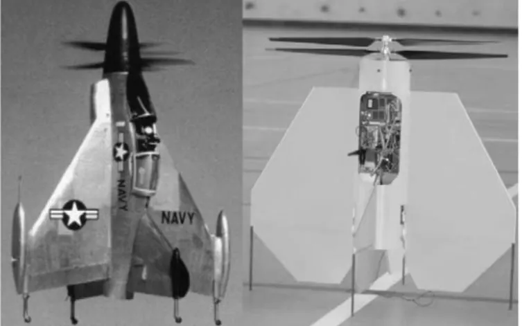
Vertigo is a VTOL mini-UAV prototype developed at ISAE in order to demonstrate a fixed wing MAV capacity to achieve autonomous transition between hover and fast forward flight. It was designed and built at the Aircraft Design Department of ISAE based on a successful early prototype which could perform transition and stable flight in manual mode. The source of inspiration for this
ABSTRACT
Recent developments in the field of Mini-UAVs lead to successful designs in both hovering rotorcraft and fixed wing aircraft. However, a polyvalent MAV capable of stable hovering and fast forward flight is still expected. A promising candidate for such versatile missions consists of a tilt-body tail-sitter configuration. That concept is studied in this paper both from the flight mechanics and control points of view. Developments are based on an existing prototype called Vertigo. It consists of a tail sitter fixed-wing mini-UAV equipped with a contra-rotating pair of propellers in tractor configu-ration.
A wind-tunnel campaign was carried out to extract experimental results from the Vertigo aerodynamic characteristics. A 6-component sting balance was fitted in the powered model enabling excursion in angles of attack and sideslip angles up to 90°. Thus, a detailed understanding of the transition mechanism could be obtained. An analytical model including propwash effects was derived from experimental results.
The analytical model was used to compute stability modes for specific flight conditions. This allowed an appropriate design of the autopilot capable of stabilisation and control over the whole flight envelope. A gain sequencing technique was chosen to ensure stability while minimising control loop execution time. A MATLAB-based flight simulator including an analytical model for the propeller slipstream has been developed in order to test the validity of airborne control loops.
Simulation results are presented in the paper including hover flight, forward flight and transitions. Flight tests lead to successful inbound and outbound transitions of the Vertigo.
.
Development of a VTOL mini UAV for
multi-tasking missions
B. Bataillé J.-M. Moschetta
[email protected] [email protected]
ISAE France
D. Poinsot C. Bérard A. Piquereau
[email protected] [email protected] [email protected]
ONERA DCSD and ISAE France
disk and the wing dimensions. However, it will lead to aerodynamic coefficients 22% bigger than if they were obtained by using the actual wing area which is equal to 0·24m². Although lateral charac-teristics were studied and are relevant for stability analysis, mainly longitudinal results will be presented in the following as they are believed to be the most important in regard to transition.
2.1 Unpowered tests
Preliminary tests consisted of an unpowered configuration. This was achieved by removing propellers from the propulsion unit. Tests were run for several speeds: 5, 10, 15 and 20m.s–1.
2.1.1 Lift
As expected, lift at zero degree angle-of-attack is zero. The wing lift coefficient reaches its maximum value of 1·1 for 23° AoA and from then gradually decreases until 90° where the lift is zero (Fig. 4). A progressive separation starts at 15° where the lift slope begins to decrease. A sharp stall occurs at 23° AoA where the lift slope sign becomes negative. Yet, it should be noticed that the lift coefficient remains greater than 0.8 up to 55° AoA. In the low angle-of-attack portion of the diagram, the lift slope shows noticeable non-linearity typical of small aspect-ratio wings and especially delta wings. This non-linearity attributed to vortical structures can be taken into account using Polhamus formulation of the lift coefficient:
CL= KPSin α Cos
2α + K
vCos α Sin
2α . . . (1)
where Kp depends on the aspect ratio, sweep angle and leading
aircraft is the Convair XFY-1 Pogo prototype (Fig. 1). The airframe consists of two flat plate wings of which polygonal planform approximates the inverse Zimmermann wing and two vertical fins that are symmetrically placed on either side of fuselage. Two-bladed contra-rotating propellers are mounted in tractor configu-ration.
It is fitted with two large flaps on each wing to ensure enough control efficiency in hover. Although each propeller is powered by its own electric motor, the choice has been made to apply the same throttle to both motors. The wingspan is 650mm and the propeller diameter 500mm (Fig. 2). All the hardware is fitted inside the cylin-drical shaped fuselage. The prototype mass is m = 1·6kg fully equipped and its centre of gravity lies 145mm behind the leading edge. More details about the system architecture can be found in Ref 1.
2.0 AERODYNAMIC AND PROPULSION
ANALYSIS
In order to analyse flight in the transition regime and obtain an accurate aerodynamic model, a full scale model of Vertigo was tested in an open loop low speed wind tunnel. It was fitted on a 6-component sting balance and placed in the centre of the 3m x 2m elliptical test section (Fig. 3). The piloted arm linked to the sting balance enabled to explore angle-of-attack and sideslip angle up to 90° so as to obtain longitudinal and lateral aerodynamic parameters. In the following, the choice has been made to use l = 0·5m as a reference length and a reference area corresponding to the 500mm-diameter propeller disk as it is both representative of the propeller
Figure 1. Pogo (left) and Vertigo (right) prototypes. Figure 2. Vertigo detailed geometry.
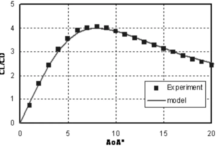
Figure 5. experimental data and model comparison for lift. Figure 6. induced drag model and experimental data comparison.
Figure 7. Lift-to-drag ratio experimental values and model comparison. Figure 8. Pitching moment coefficient at the centre of gravity from – 10° to 90° AoA.
Figure 9. Lamar model and experimental data of pitching moment coefficient at leading edge.
edge shape of the wing. It represents the potential lift contribution. Coefficient Kvis a constant factor usually equal to π which
repre-sents the vortex lift contribution. With Kp = 2·6 and Kv = 1·25,
Equation (1) is in good agreement with the experimental data up to 15°, confirming the existence of vortical structures on the leeward side of the wing. The value of Kv greater than π is only
due to the reference area choice as explained earlier. Polhamus formulation is compared with experimental data (Fig. 5) for moderate angles of attack. Good agreement is found between both until early separation at 15° AoA.
2.1.2 Drag
The lift to drag curve presents a very clean parabolic shape until stall. The minimum drag coefficient is reached at 0° AoA and its value is CD0 = 0·054. This rather high value can be attributed to
the base drag and the nose drag of the cylindrical fuselage. After stall, drag increases until a maximum value of 1,5. It is common practice to express drag as the sum of the minimum drag and the induced drag as:
CD= CDo+ Ki · CL
2 . . . (2)
with CLbeing described as above in Equation (1) and the induced
drag coefficient whose value Ki= 0·29 was found to best fit the
experimental results until separation (Fig. 6).
Computing the lift-to-drag ratio using Equations (1) and (2) leads to a reasonable accuracy compared to experimental values. An error smaller than 2% is made over the non stalled AoA range from 0° to 20° (Fig. 7). A maximum ratio of 4 is found at 8° AoA.
2.1.3 Pitching moment
The pitching moment coefficient at the expected centre of gravity CG, located 145mm behind the wing leading edge, has been measured over the range –10° to 90° angle-of-attack (Fig. 8). Three parts can be pointed out on this curve: the first part that goes from –5° to +5° indicates a linear behaviour for low angles of attack where the aerodynamic centre stands ahead of the CG. This suggests that the centre of gravity should be slightly shifted upstream in order to remove instability at small incidence. The second part starts at 15° when the slope becomes negative, due to the onset of separation on the leeward side of the wing. One can notice that the pitching moment vanishes with a stable slope around 15°, that is 8° before the wing stall angle (23°). This suggests that the wing stall is dominated by the vortical lift that shifts the centre of lift further downstream. The third part begins right after the stall angle with a pitching moment slope which tends to decrease and to become constant up to 90° angle-of-attack.
It is obvious that a linear model would be unable to accurately represent this behaviour over a large enough range of incidence. Lamar's nonlinear equation for the pitching moment at the leading edge can be used to take into account this non-linearity:
–(Cm)LE= xpKpSin α Cos α + xeKv·Sin
2α
. . . (3) where xpis the adimensioned distance from the leading edge along
the chord wise direction at which the potential linear lift is assumed to be acting. xe is the location at which vortex lift is
assumed to act. Linear lift is assumed to act at 25% of chord (which seems correct judging by pitching coefficient at CG for small incidence), therefore xp = 0·25. A value of xe = 0·4 was
found to best fit experimental points (Fig. 9) which is in agreement with results found by T.J. Mueller et al² for this kind of wing planform. Kpand Kv are the coefficients already introduced
in Equation (1).
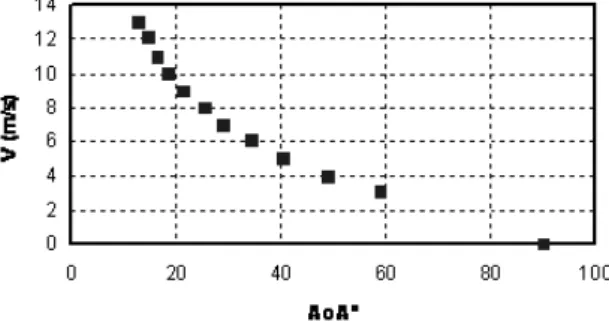
Figure 11. Speed (ms–1) vs aircraft AoA° over transition.
Figure 12. Input Power(W) vs aircraft AoA° over transition.
Figure 14. Pitching moments at CG vs aircraft AoA° over transition.
Figure 15. Velocity triangle at the propeller disk. Figure 13. Vertical forces vs aircraft AoA° over transition.
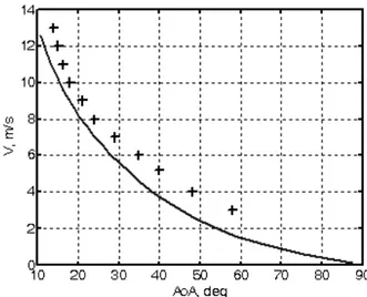
regimes can be distinguished: the first part that goes from 13° to 20° corresponds to cruise flight with speeds from 13ms–1to 9ms–1. The
second part corresponds to transition and lies approximately between 20° and 50°. The last part starts from 50° until 90° and corresponds to hover flight and slow translation where speed is lower than 4ms–1
. The relatively small maximum speed for such a mini UAV is mainly due to the propeller small fixed pitch that was set to improve hover flight performance.
3.2 Power
Electrical input power was measured in powered tests (Fig. 12). Voltage was held constant at 11·1V for both motors. A minimum input power of about 95W is found for a 10ms–1speed at 19°. Power
slowly increases towards hover flight until a maximum power of 170W. Power increases sharply toward fast flight with a local maximum of 130W at 13ms–1.
3.3 Forces
Although not plotted on Fig. 13, the aircraft horizontal force was found to be oscillating around zero (± 0·02daN) along the transition test confirming equilibrium on the horizontal axis. Vertical aircraft force is approximately equal to 1·6daN which corresponds to the Vertigo weight. It can be seen that the propellers vertical force contribution rises in a regular manner during transition and repre-sents half of the aircraft force at 40° AoA. In hover flight, propeller thrust is higher than aircraft thrust as the resulting vertical force generated by the airframe is a parasite drag due to the propeller slipstream over the wings. Assuming that there is little influence of the wing on the propellers, the wing vertical force can be deduced by subtraction between aircraft and propeller vertical forces. Yet, the resulting force is much larger than the force that would be computed from the model developed in the first part using the free stream dynamic pressure and angle-of-attack. Such a large force can be explained by a strongly modified flow passing through the propeller disk and impacting the wing. This strong influence of the propeller on the wing aerodynamic needs to be taken into account to predict transition and a simplified method to do this will be presented in the next subsection.
3.4 Pitching moments
The resulting aircraft pitching moment at CG is positive all along transition until hover flight where it becomes negligible. It is the opposite of what could be expected by considering the pitching moment value of the wing alone for this incidence range. Nevertheless, it should be noted that the propeller pitching moment is even greater and thus confirms that the wing may indeed produce a pitch-down moment during the transition. The propeller pitch-up moment is in fact due to a parasite force acting at the centre of the propellers and normal to the thrust line. This ‘side’ force due to a propeller with angle-of-attack will be discussed at the end of the next subsection. It will be shown in the flight dynamics section that a moderate positive throw of elevons can balance this pitch-up moment.
3.5 Conclusion
The Vertigo transition was simulated in the wind tunnel. It showed that steady states could exist for speeds from 0 to 13ms–1. However
no assumption relevant to stability of these steady states can be worked on at this point. The deduced wing vertical force highlighted a strong influence of the propeller flow on the wing aerodynamic. Furthermore, a parasite propeller ‘side’ force was identified to have an important effect on the pitching moment of the aircraft. These two phenomena appear to be of great importance in regard to transition and hence need to be investigated.
2.1.4 Flaps efficiency
The pitching moment coefficient derivative with respect to elevons
Cmdmwas investigated. Several elevons deflection angles dm from –30°
to 30° were tested for the full range of incidence (Fig. 10).
The flap efficiency was found to be rather constant over a large range of incidence even beyond stall. Yet, flap efficiency starts to decrease after 40° AoA and especially for positive flap deflection. A linear slope Cmdm= –0·32 was found to be a good approximation of
flap efficiency in the range of dm between –30° and 30°. A similar investigation was lead for the lift coefficient derivative with respect to elevons CLdm. Again, results showed a constant flap efficiency in
generating additional lift over a large range of incidence. A linear slope CLdm= 1·1 was found to best describe elevons effect on lift.
2.1.5 Conclusion
The longitudinal aerodynamic properties of the unpowered Vertigo were presented for a range of incidence from –10° to 90°. Strong nonlinearities specific of low-aspect ratio wings were observed. These nonlinearities can be attributed to progressive separation and creation of vortical structures on the leeward side of the wing. A nonlinear model based on Polhamus and Lamar equations of lift and pitching moment coefficients was developed to fit experimental results accurately up to 20° AoA which is the limit before stall. Although it has not been presented here, lateral properties were also investigated with sideslip angle exploration from –10° to 90°. The resulting model is very similar to the longitudinal one as the vertical fins act in the same manner as the wing when in sideslip. Due to the symmetry of the aircraft, some aerodynamic coefficients such as roll torque due to sideslip coefficient were indeed found to be negligible.
3.0 POWERED MODEL TESTS
In order to study the behaviour of the Vertigo in transition flight, specific wind-tunnel tests were conducted in conditions representative of level flights. A minimum speed of 3ms–1
could be set in the wind tunnel without too many fluctuations and no steady state could be reached at 14ms–1and beyond, because of power limitation. Therefore
equilibrium states starting from hover (0ms–1) up to 13ms–1 were
simulated in the wind tunnel with a speed interval of 1m/s, except for wind speeds of 1 and 2ms–1, for which the free stream flow would
become unsteady. The following data acquisition procedure was applied:
1. A given wind speed chosen in the range 0 to 14ms–1was set in
the wind-tunnel.
2. Throttle and angle-of-attack were iteratively set so as to obtain equilibrium values of vertical and horizontal forces corre-sponding to a steady flight: no drag force and a lift force of 1·6kg.
3. At that particular combination of free stream speed, throttle and angle-of-attack, aerodynamic forces and moments were measured.
As the flaps could not be set in real time, it was chosen to set them at 0° for the whole test and to measure the resulting pitching moment. Once these tests were done, a second series of tests at equilibrium conditions were done with the wings removed. Assuming that there is little influence from the wing onto the propellers, it was then possible to separately quantify the propellers contribution and the airframe contribution over transition. The main results are plotted in Figs 11 to 14.
3.1 Speed
As mentioned earlier, steady states were found for every speed from 0 to 13ms–1
Because it is more convenient to obtain equations valid also for hover flight, the induced velocity which would be induced statically for the same thrust is used as the reference:
Therefore Equation (6) can be written in dimensionless form:
Solving this equation leads to the induced speed for any given (T,V,α). However this polynomial equation admits ‘obvious’ roots only for the specific cases of α = 0° , α = 90°:
If α = 0° then
If α = 90° then
For the other incidence values, Equation (8) can be solved numeri-cally. It is then straightforward to obtain the total accelerated slipstream velocity value and the associated slipstream angle-of-attack.
From Fig. 16, slipstream resulting velocity VR can be written:
and the slipstream angle-of-attack:
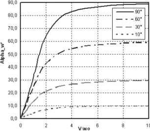
As the wing is aligned with the thrust line, the effective wing angle-of-attack αw is simply equal to:
αw= α – αs
The evolution of αw as a function of speed is plotted for several aircraft incidence values in Fig. 17.
Although this model is very simplified, computation of wing forces using above VRand αw gives results close to the observed
experi-mental forces. A model taking into account span wise and chord wise velocity and angle variation should yet be developed so as to describe more accurately propeller and wing interaction. It would be necessary for aerodynamic design and analysis but the presented model is repre-sentative and simple enough to be used for simulation purpose.
4.2 Propeller parasite forces and moments
A single propeller with no incidence produces a single thrust force and an associated torque on the roll axis. In the case of the Vertigo propulsion system, the contra-rotating propellers produce thrust and a very low torque that is negligible. A propeller in incidence (or a rotor in forward flight) will produce two additional efforts.
a yawing moment known as the p-factor. This moment is due to the difference in loading between the advancing blade and the retiring blade relative to the tangential component of the speed to the propeller.
4.0 PROPELLER IN INCIDENCE
Most propeller theories are developed for the ideal condition in which the incoming speed is aligned with the thrust line of the propeller. Yet, most aircraft encounter flight conditions such as take off or low speed where the propeller disk is at incidence. It is especially the case for tilt-body aircraft whose propellers incidence may reach 90° during transition. This incidence will have effects on the flow behind the propellers and on the forces and moments produced by the propellers.
4.1 Propeller flow
In order to take into account the free stream angle-of-attack and dynamic pressure modifications through the propellers, the choice is made to consider the propellers acting as an actuator disk. This way, the momentum theory can be applied and corrections can be made to account for the effect of incidence following McCormick(3).
At the plane of the disk, a velocity w is induced and thrust can be written:
T = 2ρAV′w . . . (4)
where ρAV′ is the mass flow rate through the disk and 2w the
ultimate change in velocity of the flow. V' can be expressed as:
V' =
[
(V Cos α + w)2+ (V Sin α)2]
½ . . . (5)Equation (5) developed in (4) gives:
Figure 16. Velocity triangle of fully accelerated slipstream.
Figure 17. Effective wing angle-of-attack as a function of speed for a constant thrust.
. . . (6)
. . . (7)
. . . (8) α
compute longitudinal equilibrium using a MATLAB-based algorithm. In this case the first value defined by operator is the aerodynamic speed V. The efficiency of the solver algorithm to converge toward the solution is very fine: the relative error is always smaller than one by a million.
The aerodynamic equilibrium speed during transition is plotted in Fig. 20. The computational results are in good agreement with the wind-tunnel measurements (Fig. 11 and discrete points in Fig. 20). Since a level flight is assumed during transition, the angle-of-attack α also represents the aircraft’s pitch angle.
a drag force that was called earlier ‘side force’ in the powered tests section. This force is located inside the plane of the propeller and is opposed to the tangential speed component. It is due to the difference in drag between the advancing blade and the retiring blade.
In the case of contra rotating propellers, the p-factor is negligible as the yawing moment produced by each propeller will balance one another. On the contrary, drag forces will add to each other. Detailed analysis of these efforts were lead by Herbert S. Ribner(4)in the case
of propellers in yaw. However, the developed formulas are only valid for small values of yaw. A simpler analysis made by Glauert(5)
leads to a quite simple formulation of the drag force that will be noted Np:
with J the advance ratio of the propeller, Cpits power coefficient.
Still, this equation is only valid for small angles-of-attack. Another equation based this time on helicopter airscrew in forward flight is also proposed by Glauert(5):
with B the number of blades, c the average chord, ρ the air density, Ω the rotation speed, R the propeller radius, CDthe blade profile drag
coefficient, θ the blade pitch angle and μ the non dimension induced velocity. Because of a lack of experimental data about the Vertigo propeller such as Cp(J) characteristics or accurate drag data, these
formula cannot be used in this study. They would lead to too small normal force value. An empirical formula matching experimental values of Npwill be used in the model instead.
4.3 Conclusion
Aerodynamics and propulsion analysis was lead on the Vertigo model. Non linear behaviour of the wing was observed and an adapted model was developed. Powered tests revealed a strong influence of propeller flow on the wing. Moreover, a propeller drag force due to incidence was found to be responsible for a pitch-up moment in transition. A simple model of propeller flow was presented and some analysis of the propeller drag force was found in literature. The developed models will be used in the next part for stability and control purpose.
5.0 FLIGHT DYNAMICS
Based on the previous analysis of aerodynamic and propulsion forces and moments, a longitudinal model for the tail-sitter Vertigo has been derived. The flight dynamics model includes the propwash effect and the propeller-wing interaction which proved to be essential to adequately describe transition. With the present model a family of trajectories have been simulated and analysed and the evolution of the dynamic behaviour of the Vertigo during transition is presented in a pole-map diagram. The trajectory simulation will be used for the design of control laws at several flight points in the speed range of 0 to 13ms–1. Then, elements around the stability
between discrete points will be getting onto.
In Fig. 18 definition of the different forces and velocities are presented following McCormick's approach(3) for the definition of
the induced velocity at high angle-of-attack. In the present model, the velocity VR resulting from the combination of the free stream
velocity and the induced velocity impinges the wing with an effective angle-of-attack αwwhich defines the aerodynamic frame of
reference. A system of 10 equations presented in Fig 19 is used to
Figure 18. Forces and Velocities definition for equilibrium.
Figure 19. System to solve the longitudinal equilibrium.
Figure 20. Equilibrium speed during transition (cross: wind-tunnel data, solid line: computed).
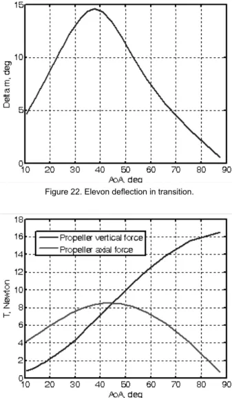
wing effective angle-of-attack over the transition phase. This remains within the domain of validity of the aerodynamic model. Another important result is obtained from the evolution of the elevons deflections necessary to guarantee the longitudinal equilibrium around the pitch axis (Fig. 22). First, the maximum value of elevons deflection never exceeds the maximum deflection angle of 30°; second, one can notice a rapid inversion of the slope over the transition. So far, only equilibrium states have been considered. In the following section, a modal analysis is applied in order to draw conclusions on flight stability during transition.
6.0 CONTROL LAWS DESIGN
6.1 Introduction
For a classical aircraft in forward flight, longitudinal and lateral decoupling and control design are proved and used to simplify the processes. There are five lateral state variables [v,r,p,φ,ψ]; these signals can be used to drive the two lateral controls δlaileron and
rudder δn. There are five longitudinal state variables [u,w,θ,q,h] these
signals can be used to drive the two longitudinal controls elevon δm
and thrust δx.
Figure 21 illustrates the effective wing angle-of-attack during transition. A maximum value of αw≈ 20° is observed for α = 32°
which indicates that the wing never stalls during transition since the wing stall angle is 23° (Fig. 4).
In the Fig. 22, elevons deflection values in transition are shown. They correspond to the evolution of the longitudinal moment during the transition. The rapid variation of the moment is due to the evolution of the propeller normal force Npand the nonlinear Cm(CG).
The Np force effect is observed here with the creation of a major
positive moment. An important result is about the maximum value of the elevons deflection of about 14° which is relatively small compared to the aircraft’s saturation value of 30°.
Figure 23 represents the total slipstream velocity VRas seen by the
wing during transition. It can be observed that a minimum value of the relative speed VRis reached for a free stream velocity of V =
4.5ms–1
which corresponds to an angle-of-attack α = 34°. Fig. 23 illustrates the importance of the slipstream contribution on the actual relative velocity as seen by the wing.
Figure 24 shows, in comparison with results from the wind-tunnel analysis (Fig. 13), that the vertical contribution of the propeller force gradually increase during transition while the horizontal component reaches a maximum value at about 40° angle-of-attack
Figures 21 to 24 illustrate the complex behaviour of the different contributions during a balanced transition. One of the most important results concerns the relatively low maximum value of the
Figure 21. Wing effective angle-of-attack AoAwin transition. Figure 22. Elevon deflection in transition.
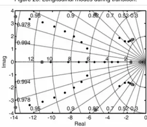
The large blue cycle plot is for equilibrium at 0·1ms–1 and the
large red cycle is for equilibrium at 13ms–1
. The evolution is shown by different points. The evolution’s rate is observed by the gap between two points. One can see here under the eigenvalues of the matrix for 0·1 and 13ms–1.
Between this two values of λ, a smoothly evolution can be
observed, displayed in the Fig. 25. The most important result of this analysis is the constant natural instabilities. The principal reason of that is the position of the centre of gravity in the Vertigo.
To conclude this part, a general longitudinal state space analysis was made with the roots values observation of the dynamic matrix. The principal result is the important variation of the natural dynamic comportment during the transition.
Conventionally the aeronautics community uses the body-refer-enced Euler angles (φ,θ,ψ) to relate the inertial and body reference frames of an aircraft. This representation works well for attitude estimation and controls, if pitch and roll angles are relatively small. From investigation it can be seen that the described set of Euler angles contains a singularity in the kinematics equations when φ approaches positive or negative π/2 known as gimbals’ lock (ψ and φ are not unique).
These equations are integrated over time for attitude estimation, resulting in a divide by zero in the described conditions. Moreover, elevator control based upon error in θ and rudder control based upon error in ψ degrades as φ and θ become larger than π/4. Hence, it is clear that a tail-sitter, which is intended to fly both vertically and horizontally, is incompatible with the conventional attitude represen-tation.
In the Vertigo autopilot the state observation and estimation is made by several sensors’ fusions. Sensors are GPS, IMU, Static Pressure and Ultrasonic for the ground detection. The large flight envelope and equilibrium possibilities of this aircraft impose the use of quaternion theory for space orientation calculation. So, 13 states are used for the control: body frame velocities [u,v,w], rate gyros [p,q,r], earth frame position [x,y,z] and space orientation [LQ0,Q1,Q2,Q3,Q4].
First, for Vertigo aircraft and its transition objectives, a point about state dynamic coupling has to be discussed. Augmented classical equations are used for the modeling as it is done in Boiffier(6)
. A modification is brought to the velocity as it can be seen in Figs 18 and 19 which is used to compute aerodynamic forces and moments. Therefore classical longitudinal-lateral decoupling can be applied. However the use of quaternion for the space orientation creates a coupling between equations. In this paper, only a longitu-dinal analysis has been led.
7.0 STATE DYNAMIC VARIATION
ANALYSIS
The equilibrium analysis showed that a continuum of equilibrium points existed and now a study of the longitudinal dynamic comportment can be led.
The classical state space representation is defined below:
X = AX + Bc . . . (13)
Here X is the state vector, c is the control vector A and B and are constant system matrices. The state vector for the longitudinal system is:
X =
[
Δu Δw Δϑ q Δz]
. . . (14)The longitudinal control vector is:
cT= [δ
x δm] . . . (15)
Although relatively small departures from the steady state are thereby restricted, these responses are nevertheless extremely useful and informative. And in this part a particularly focus of the eigen-values of the matrix is presented, because they give information about stability and natural dynamic comportment (rapidity, damping).
To understand the dynamic comportment in transition we computed a family of state space model:
X = AiX + Bic . . . (16)
With Aiand Bisystem matrices for the equilibrium velocity V = i. In
the Fig. 25 evolution of the pole in a pole-zero maps is observed, with beginning to 0·1ms–1
and finishing at 13m/s with a 0·2ms–1
step value.
.
.
Figure 25. Longitudinal modes during transition.
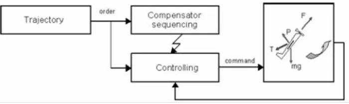
The d) and e) process part, calculated on line and during the flight, are used to control the system in the entire flight envelope and are detailed in Fig. 27. An order arrives from trajectory algorithm in term of V airspeed velocity to follow. The interpo-lation sequencing algorithm is used to compute the good value of GS gain and ES equilibrium with lookup table and linear interpo-lation. For the equilibrium a computation is made for determining the good value of each state order for example in longitudinal the state is represented by Equation (16) and for the u body velocity the difference δu = ESδu– uobsis calculated in each time with ESδu
from trajectory table interpolation. Second source of ES sequencing is for the control order generation, with the summation part after DC = [δx δm], to ensure the good value of throttle and
elevator to respect the trajectory order.
The general autopilot structure is shown in Fig. 28, and tries to explain the control strategy. An open loop trajectory is defined off line to minimise one or many criterion (for instance to minimise the altitude variation during transition, minimise structural constraint (minimise acceleration) or minimise the total time of transition.
It is interesting to determine the degree of stability of the gain-scheduling control strategy. Fig. 29 shows a trajectory order in transition, black points are discrete point of K(i) feedback control point determination from ground velocity desired value V = i. The objective is to determine the hardiness of a feedback design to a parametric variation (here velocity). To determine the robustness of a feedback design to a parametric variation (here velocity), the μ – analysis, G. Balas(9)
, can be used. Of course, to use this technique, an LFT modelisation(12)must be obtained.
9.0 SIMULATION AND FLIGHT TEST
Some simulation results from a Matlab-based simulator are presented in this section. This simulator includes all the equations and comportment of the Vertigo aircraft, with in line propeller flow computation, non linearity, noise and actuators limitations.
8.0 FEEDBACK CONTROL DESIGN
Lots of feedback control designs are made for this kind of system, for example Osborne(7)uses model reference adaptive controller and
Knoebel(8)uses adaptive quaternion control, for their VTOL aircrafts,
both from non linear control design.
Here, gain sequencing technique based on multi-linear system is presented. Below, process to compute gain scheduling is described: a) Analytical linearisation [A(x), B(x), C(x), D(x)]
b) Flight envelope cutting [A(i), B(i), C(i), D(i)] c) In each point, linear Gain computation
[
K(i)]
d) Equilibrium calculus
[
ES]
e) Gain sequencing
[
GS]
The analytical linearisation described for longitudinal motion in the precedent state space analysis, is computed with a Matlab-based algorithm using maple software. The result is a complete analytical state space system valid for the entire flight envelope, with first order derivative approximation.
The second of this gain-scheduling process is the choice of discrete points of linearisation from ground velocity desired value
V = i. For longitudinal equilibrium the system shown in Fig. 19 is
used, and it permits to determine initial condition for all the state and replace analytical equation by numerical values to create a family of state space model [A(i), B(i), C(i), D(i)].
In each V = i point, K(i) is calculated, to stabilise the system, with this control law: c = –Kx, to compute the K(i) feedback gain family an linear quadratic algorithm has been used with the same function
cost to minimise and same value for Q and R
matrices. The result of the closed loop eigenvalues evolution (roots of the ACLmatrix with ACL(i) = A(i) – B(i)K(i)) during transition is
shown in Fig. 25. It’s interesting to observe the evolution of these roots, with V = 1 in blue circle, V = 13 in red circle and other in black point. One can notice that the damping of the closed loop remains acceptable for the whole speeds considered.
Figure 27. Sequencing. Figure 28. General autopilot structure.
This simulator is linked to an embeddable control code in order to test control law before real flight test. Two mixed control laws are used here for this simulation. The first is gain sequencing feedback control, presented in precedent section, and the other is feedback control loop especially designed to realise and hold the hover flight. This second control loop is discussed in Refs 1 and 10. During transition from 13 to 3ms–1longitudinal gain scheduling method is active and from 3ms–1to
hover flight a hierarchical axis by axis control loop is used, better to hold earth frame position than classical coupling state method. At 3ms–1
a commutation method is applied.
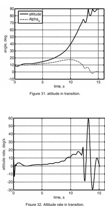
Figure 30 shows velocities in transition with a linear non optimised open loop trajectory order. Figure 31 shows attitude in transition, first in continuous curve we observe a smooth modification of the pitch from ≈10° to ≈70° and after one short oscillation phase corresponding to commutation between longitudinal control low and hold over flight. Dashed curve corresponds to the effective wing angle-of-attack αw, its
comportment follows equilibrium calculus in term of maximum value always inferior to 20°. αwbegins at the same value than the pitch in
level flight, and finishes close to zero, corresponding to hover flight in second 15.
Figure 32 shows the attitude rate in transition in constant augmen-tation with limited value from 0 to 13s, and after two important oscilla-tions due to the commutation between control laws. A work about method of commutation can be led to minimise amplitude; however this oscillation was quickly damped by control low.
Figure 33 shows the aircraft altitude value during transition, a total variation of six meters can be observed, in this simulation the altitude was not hold to a specifically value a work can be made about trajectory. But this ‘natural’ trajectory is interesting because Stone(11)in
his work about optimisation of transition finds this kind of trajectory. Concerning real flights, numerous campaigns was led with the aircraft, in different configuration and background, indoor for attitude and altitude automatic hover-flight test, indoor for primary test of transition with gain-scheduling (two different gain during transition) but under manual control for velocity and position, outdoor for attitude stabilised flight under manual control. Campaign to test the full autonomous transition control configuration presented here in simulation should be lead in spring and summer 2008.
10.0 CONCLUSION
A complete study about the Vertigo VTOL tail-sitter mini-UAV has been carried out. Aerodynamic and propulsion effects have been measured in a low-speed wind-tunnel and a full longitudinal flight model valid up to the stall angle has been developed for the simulation of transition. In particular, a simple but realistic propwash model has been adapted and used to describe the transition mechanism. The equilibrium analysis proved the feasibility of performing transition with the Vertigo prototype with the introduction of the effective wing angle-of-attack αw. The flight model has been used to design control laws and
analyse stability issues. Finally a control design based on a gain-sequencing technique and commutation was used with the assumption of a good knowledge of the dynamic behaviour during transition. Simulation of transition under automatic control has been proposed in view of preparing future flight tests experiments
ACKNOWLEDGMENTS
The authors would like to thank the S4 wind-tunnel technical staff for their support and expertise all along the wind-tunnel campaign. The authors wish to thank the technical staff of the Department of Aerodynamics and Propulsion. They would also like to acknowledge dedication to the Vertigo project of Dominique Bernard from CAS (ISAE Aerospace Center). The present work has been partly funded by the French Armament Procurement Agency (DGA) under grant 06.60.033.00.470.75.01.
Figure 31. attitude in transition.
Figure 32. Attitude rate in transition.
CONTACT
Boris Bataillé, PhD candidate, Department of Aerodynamics, Energetics and Propulsion (DAEP), Institut Supérieur de L’ Aéronautique et de L’Espace (ISAE). BP54032, FR-31055 Toulouse Cedex 4, France, [email protected]
Damien Poinsot, PhD candidate, Department of Flight Dynamics and Systems Control, ONERA-DCSD BP 74025 and Department of Mathematics, Computer Science and Control Theory, ISAE BP54032, FR-31055 Toulouse Cedex 4, France, [email protected].
Jean-marc Moschetta, Professor, Department of Aerodynamics, Energetics and Propulsion (DAEP), Institut Supérieur de l'Aéronautique et de l'Espace (ISAE). BP54032, FR-31055 Toulouse Cedex, France, [email protected]
Caroline Bérard, Professor, Department of Flight Dynamics and
Systems Control, ONERA-DCSD BP 74025 and Department
of Mathematics, Computer Science and Control Theory, ISAE BP54032, FR-31055 Toulouse Cedex 4, France, [email protected]
Alain Piquereau, Research Engineer, Department of Flight Dynamics and Systems Control, ONERA-DCSD BP 74025 FR-31055 Toulouse Cedex 4, France, [email protected]
REFERENCES
1. BATAILLÉ, B., POINSOT, D., THIPYOPAS, C. and MOSCHETTA, J.M. Fixed-wing micro air vehicles with hovering capabilities, NATO RTO meeting, AVT-146, Symposium on Platform Innovations and system integration for unmanned air, land and sea vehicles, Florence, Italy, 14-17 May 2007. 2. MUELLER, T.J., KELLOGG, J.C., IFJU, P.G. and SHKARAYEV, S.V.
Introduction to the design of fixed-wing micro air vehicles, AIAA Education Series, AIAA, 2, 2006.
3. MCCORMICK, B.W. Jr., Aerodynamics of V/STOL Flight, Dover Publications, Inc, NY, USA, 1999.
4. RIBNER, H.S. Propellers in yaw, NACA Rept 820 1943.
5. DURAND, W.F. Aerodynamic Theory, IV, Julius Springer, Berlin, Germany, 1934.
6. BOIFFIER, J.-L. The Dynamic of Flight: The Equations. Wiley, ISBN 0471942375
7. OSBORNE, S.R. Transitions Between Hover and Level Flight for a TailSitter UAV. Master of Science, Department of Mechanical Engineering. Brigham Young University, December 2007.
8. NATHAN, B. Knoebel. Adaptive quaternion control of a miniature tailsitter UAV. Master of science, Department of Mechanical Engineering. Brigham Young University. December 2007.
9. BALAS, G., DOYLE, J.C., GLOVER, K., PACKARD, A. and SMITH, R. Analysis
and Synthesis, MUSYN, and The Mathworks, Inc., 1991.
10. POINSOT, D., BÉRARD, C., KRASHANITSA, R., and SHKARAYEV, S. Investigation of flight dynamics and automatic controls for hovering micro air vehicles. In submission in AIAA Guidance, Navigation and Control Conference 2008, Hawaii, USA.
11. STONE, R.H. and CLARKE, G. Optimization of transition manoeuvres for a tail-sitter unmanned air vehicle. Preprint report.
12. MAGNI, J.F. Extension of the linear fractional representation toolbox (LFRT). In Proceedings of the IEEE International Symposium on Computer aided control system design, Taipei, Taiwan, pp 261–266, September 2004.