Annex 60 : subtask 2.2

(1)

1

U

NIVERSITÉ DE

L

IÈGE

FACULTÉ DES SCIENCES APPLIQUÉES

DÉPARTEMENT D’AÉROSPATIALE ET MÉCANIQUE

LABORATOIRE DE THERMODYNAMIQUE

Preliminary report

Kevin SARTOR

July 2015

(2)

2 Université de Liège

Campus du Sart Tilman, B49 Quartier Polytech 1,

Allée de la découverte,17 B-4000 Liège

Belgique

Contact: Kevin Sartor

(3)

3

Table of content

1 INTRODUCTION ... 4

2 MODELING METHODS ... 5

2.1. Modelica implementation (finite volume method) ... 5

2.2. Modelica alternative implementation ... 7

2.3. Comparison of modeling approaches ... 8

2.4. Matlab implementation (plug flow) ... 10

3 PERSPECTIVES ... 13

(4)

4

1 Introduction

One subtask of the Annex 60 (Task 2.2) consists in the modeling of district composed by thermal and electric networks. In this contribution, several modeling techniques are investigated to assess the behavior of the thermal part of the district heating network. These modeling techniques are compared to find the best modeling approach.

A district heating network (DHN) is composed by several pipes to connect power plant(s) to end-users (residential buildings, industries, etc.). The length of the pipes in the network can vary from a few meters up to several kilometers for the largest DHN. For such pipes, the fluid velocity is generally reduced (0.5 – 5 m/s) to limit the pressure losses [1]. Therefore, the energy supplied by a power plant could take minutes to hours to reach the farthest end-users.

The modeling of heat transport in DHN is useful:

- To design correctly the DHN itself (pipe diameter, operating temperatures, etc. ) in order to ensure comfort in buildings and minimize the investment costs;

- To investigate control strategies of DHN and the related power plants to reduce energy consumption, emissions and costs;

- To reduce the investment costs related to the control strategies by avoiding the use of sensors (mass flow rate, temperature,…).

In order to reduce the energy losses and/or to perform a useful control of the DHN, two main phenomena should be considered:

- Heat losses: the larger the operating pipe temperature, the more heat losses. Therefore, as much as possible, the pipe temperature should be decreased to reduce heat losses while ensuring thermal comfort in the farthest buildings;

- Pumps consumption: in first approximation, the electric pump consumption is related to the mass flow rate by a quadratic law.

These two aspects are related. Indeed, if the supplied pipe temperature of the DHN is reduced, the mass flow rates have to be increased because of the lower limit on the return pipe temperature to ensure buildings comfort.

(5)

Annex 60: subtask 2.2 Modeling heat transport in district heating networks

5

2 Modeling methods

Models available in the Modelica or external libraries are first studied to determine the advantages and the disadvantages of using them for the modeling of the heat transport in district heating networks.

2.1. Modelica implementation (finite volume method)

In the Modelica library, a reference pipe is modeled by a one dimensional finite-volume approach (referenced 1D FVM). The pipe is discretized along its longitudinal axis in a finite number of cells of equal volume V, as depicted for the one-dimensional problem in Figure 1.

Figure 1. Discretization of the pipe in cells and representation of the variables [2].

In Figure 1, stands for the enthalpy; ρ for the fluid density; for the mass flow rate; for the heat flux and Δx for the spatial discretization. Two types of variables are present: cell variables and node variables (at cells interface). The latter ones are indicated by subscript “su” (supply) and “ex” (exhaust), and correspond to the inlet and outlet nodes of the cell. The variables with a “*” superscript are related to the adjacent cells. To compute the node values, a discretization scheme is implemented in the cell component. In the one-dimensional finite volume approach investigated in this study, the upwind scheme is used: [2]. To consider flow reversal, a conditional statement is added in function of the flow rates at the inlet nodes:

, (1)

where when the fluid flows in the nominal direction (from left to right in Figure 1).

In each cell, conservations laws are applied, namely the mass (2), momentum (3) and energy (4) balances [3], as given hereunder for the one-dimensional incompressible flow problem:

, (2)

, (3)

, (4)

where u stands for the velocity, p for the pressure, τ for the shear stress per unit length of the flow channel, g the net acceleration and e=h+u²/2.

(6)

6 2.1.1 Numerical diffusion

The upwind scheme, previously described, is often used because it is robust and avoids numerical oscillations and divergence if a stability criterion is satisfied. This criterion is called the CFL (Courant – Friedrichs – Lewy) condition and is defined for one dimension spatial discretization by

, (5)

where , the time step in s and , the spatial discretization in m. Notice that if CFL condition is equal to 1, the exact solution of the studied problem is found by the one-dimensional finite volume method. In this case, the entering flux covers the entire cell during the time step and the lumped properties at the nodal point correspond to the properties at the interface that are obtained by the upwind scheme. If CFL value is lower than 1, the upwind scheme can induce some numerical diffusion [4]-[5] because of the fact that the entering flux does not cover the entire cell.

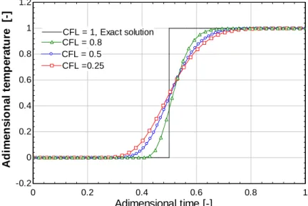
Figure 2 illustrates the numerical diffusion of the upwind scheme: in the case of a temperature step applied at the inlet of a pipe at initial time, it can be noticed that the adimensional temperature response at the pipe outlet is function of the CFL value. When CFL is lower than 1, the numerical diffusion appears: the adimensional temperature increases before the exact solution but reaches the final temperature after the exact solution. The lower the CFL value, the earlier the temperature begins to increase and the later the temperature reaches the final value.

0 0.2 0.4 0.6 0.8 1 -0.2 0 0.2 0.4 0.6 0.8 1 1.2 Adimensional time [-] A d im e n s io n a l te m p e ra tu re [-] CFL = 1, Exact solution CFL = 1, Exact solution CFL = 0.5 CFL = 0.5 CFL =0.25 CFL =0.25 CFL = 0.8 CFL = 0.8

Figure 2. The numerical diffusion due to CFL conditions for a step input for several CFL conditions.

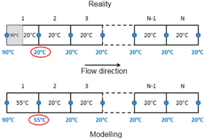
To illustrate this discussion, here is a numerical example where a fluid at a temperature of 90°C enters a pipe at a temperature of 20°C. This pipe is divided in N cells. In this example, the cell size is 1 meter and the fluid velocity is equal 0.5 m/s. In reality (superior part of Figure 5), the fluid covers only one half of the cell; therefore the outlet temperature of the cell 1 is still at 20 °C (red circle in Figure 3). However, the upwind scheme leads to a lumped temperature of the cell and the outlet temperature of the cell 1 is 55°C.

(7)

7

Figure 3 - Numerical example of the upwind scheme behaviour.

Notice that for a fixed fluid velocity, the time step is directly linked to the spatial discretization to ensure convergence. For a fixed CFL value, here 0.5, Figure 4 shows the influence of the spatial and time discretization due to the numerical diffusion. As expected, the solution is closer to the exact solution for higher spatial and time discretization but it involves a larger computational time which could be not compatible with predictive control especially for larger networks.

0 0.2 0.4 0.6 0.8 1 -0.2 0 0.2 0.4 0.6 0.8 1 1.2 Adimensional time [-] A d im e n s io n a l te m p e ra tu re

[-] Exact solution (CFL=1)Exact solution (CFL=1)

CFL = 0.5, ∆x = 10m ∆t = 5s CFL = 0.5, ∆x = 10m ∆t = 5s CFL = 0.5, ∆x = 1m ∆t = 0.5s CFL = 0.5, ∆x = 1m ∆t = 0.5s

Figure 4. The numerical diffusion due to CFL conditions equal to 0.5 for varied spatial/time steps.

Various numerical alternatives to reduce the numerical diffusion of the upwind scheme are available in the literature, such as second or higher order upwind schemes [5]–[8]. However, their use has not been investigated because they can introduce oscillations or convergence issue once implemented, especially when the level of spatial discretization is high, i.e. there is a large number of variables.

2.2. Modelica alternative implementation

In the considered case, the energy, mass and momentum balance are simplified: - It is assumed that that the section of the pipe is constant;

(8)

8 - Elevation between the inlet and the outlet pipe ( ) is not considered;

- The fluid is supposed to be incompressible (ρ is independent on the pressure); - The pressure is assumed constant inside the cell.

Equations 2 to 4 become:

(6)

, (7)

, (8)

2.3. Comparison of modeling approaches

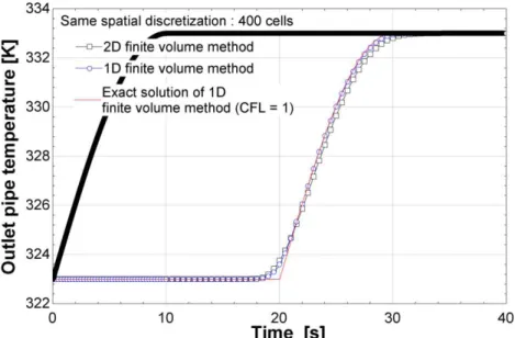
While no measurements data are available for the model validation, it was decided to consider a bi-dimensional FVM method (referenced 2D FMV) as the reference case to study the capabilities of the FVM approach. This method, available on OPENFOAM considers the radial velocity profile (the turbulence phenomenon) inside the pipe, so the pipe is discretized according to its longitudinal and radial axis. A refined discretization is used to be certain to capture the correct behavior.

A 20 meters long pipe is first considered to investigate the transport of the heat inside a pipe. This pipe has a diameter of 0.35 m1_{. The inlet temperature of the flow travelling the pipe is increased}

from 323 to 333 K in 10 seconds.

A previous study [9] showed that the 1D FVM implemented in Modelica is sufficient to model the transport of heat inside the pipe. After analysis, the 2D FVM does not bring substantial details compared to 1D FVM implemented in Modelica. The trends of the outlet pipe temperature of the 1D FVM (blue circles) and 2D FVM (black squares) are shown in Figure 5 for a cell size of 0.05 m (lower cell sizes lead to the same results). The inlet pipe temperature is depicted in straight black line. These trends are similar for the two cases. The computational time of the 2D FVM is about one hour2_{for simulating only 40 seconds. As discussed before, the pipes of real DHN are longer than 20}

meters larger; therefore it seems currently impossible to consider such refined cell discretization for a whole network with reasonable computational time. An alternative is to perform a rougher spatial discretization, i.e. increase the cell size to reduce the variables numbers and thus the model complexity. On the other hand, when the variable number increases (i.e. little cell size for long pipe), the system becomes too complex to be solved by Modelica. Indeed when a pipe of 1 km is discretized with cell size of 0.05 m, Modelica cannot initialize the simulation (for different time integrator scheme).

1_{The pipe diameter is the one of the ULg DHN with a annual heat demand of about 60MWh.} 2_{On a conventional computer with a I7 Core (2014)}

(9)

9

Figure 5 - Comparison results between 2D FVM and 1D FVM.

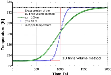
In Figure 5, the so-called exact solution of the 1D FVM (in red) corresponds to the analytical solution of the problem. Due to time and spatial discretization, problems related to numerical diffusion can occur (as discussed before). If the number of cells is reduced, some errors appear due to this numerical diffusion. In Figure 6, the cell size is increased to 1 m (blue) instead of 5 cm (green), an increase of the outlet temperature occurs sooner than it occurs in the reality. In this studied reference test case, the time difference is only five seconds but this case corresponds to a short pipe of 20 m. If a longer pipe (1 km) is considered (as shown in Figure 7), the temperature increase appears sooner compared to the exact solution of the 1D FVM.

(10)

10 0 500 1000 1500 2000 322 324 326 328 330 332 334 Time [s] T e m p e ra tu re [K ]

1D finite volume method

∆x = 100 m

∆x = 10 m

Exact solution of the 1D finite volume method Exact solution of the 1D finite volume method

Inlet pipe temperature Inlet pipe temperature

Figure 7 - Influence of spatial discretization on the results of heat transport in a 1 km pipe.

This numerical diffusion can be considered as an issue especially when the temperature variation at the pipe inlet is quick. On the contrary, if the pipe inlet temperature variation is slow, the numerical diffusion effect is reduced.

Case studies

To help the discussion, two case studies can be investigated: the Annex 60 Task 2.2 and the district heating network of the University of Liège (ULg).

In the case of the ULg DHN, the temperature variations are limited to some degrees per hour. To allow the convergence of the Modelica software and reduce the computational time, it was decided to check the resulting error obtained by the 1D FVM when a cell size of 100 m is considered. For a conventional inlet temperature profile occurring in the ULg DHN, the mean absolute square error obtained on the outlet temperature compared to the exact solution of the 1D FVM case is around 0.5K. As a result, the 1D FVM with a rough spatial discretization could be used for the modeling of the ULg DHN.

On the contrary, if the DHN uses some control strategies such as quick temperature variations or there is a night set back followed by a morning boost to ensure the comfort of buildings, this modeling method is not suitable because it induces a wrong estimation of the heat transport delay. The modeling of the district neighborhood investigated in Annex 60 cannot be solved by this approach due to the numerous pipes leading to a too complex system to solve. Even if the simplified balance equations are considered, the system still presents high number of variables. In consequence, the initialization process for Modelica remains challenging like in the previous method.

2.4. Matlab implementation (plug flow)

This alternative approach is different and based on the Lagrangian approach, i.e. the fluid particles are followed almong their direction (Figure 8).

(11)

11

Figure 8 - Lagrangian approach.

To further simplify the problem, the density of a fluid particle is considered constant during its travel along the pipe, so the mass variation inside the particle is considered equal to 0. This assumption is correct since the temperature variation between the inlet and the outlet of an insulated pipe of DHN is generally low3_{leading to a low variation of density. For each cell, an energy balance is performed}

in order to take into account the heat losses. For the sake of simplicity, it is assumed that there are no pressure losses for the considered particle. The equation system becomes:

(9) (10) While it is required to determine the pressure losses in the network in order to assess the electricity consumption of the pumps, it is proposed to lump at the end of the pipe an equivalent pressure loss as a function of the mass flow rate by means of the Darcy-Weisbach correlation.

Results of the plug flow modeling are given in Figure 9. The exact solution of the 1D FVM (dashed red line) can be obtained by simulation.

Contrary to the Modelica approach, the computation for a same spatial discretization is about 1000 times faster, allowing for a very good estimation of the heat transport delays without numerical diffusion.

3_{For example, a pipe of 35 cm diameter and 1 km length are insulated by 14 cm of mineral wool in the ULG DHN. This} leads to a temperature variation lower than 1K when the fluid velocity is superior to 0.5 m/s.

(12)

12

Figure 9 - Results of plug flow modeling.

A similar approach is implemented in Modelica under the name “spatialDistribution” but no resulting models has not been developed yet. An Annex 60 team is currently trying to implement a model to consider the heat losses with this function.

On the other hand, previous works carried out by the authors focused on the implementation of the Matlab solution in Modelica but the results have not been judged satisfactorily. One potential explanation is that the problem is linked to the time step interval and the precision used to solve the problem. When the time step (in case of resolution algorithm as Euler) is reduced and the precision is increased, the results are the same as the plug flow method available on Matlab but lead to a higher computational time. However if the time step is increased to speed up the calculations, some numerical issues appear: the tracked positions are sometimes miscalculated due to wrong approximations leading to wrong results (Figure 10).

(13)

13

Figure 10 -Results of the plug flow method implemented on Modelica

3 Perspectives

Despite the ability of the plug flow method to assess the behavior of the heat transport in heating networks, a new model is currently under development in Modelica language considering a very simple method. It assesses the transport delay of one fluid particle in function of its fluid velocity profile. The first results are promising and will be presented at the next Annex 60 meeting under the reference: “Alternative method to model the heat transport under Modelica platform”.

4 References

[1] K. Sartor, S. Quoilin, and P. Dewallef, “Simulation and optimization of a CHP biomass plant and district heating network,” Appl. Energy, vol. 130, pp. 474–483, 2014.

[2] S. Quoilin, I. Bell, A. Desideri, P. Dewallef, and V. Lemort, “Methods to Increase the Robustness of Finite-Volume Flow Models in Thermodynamic Systems,” energies, vol. 7, pp. 1621–1640, 2014. [3] J. C. Tannehill, D. A. Anderson, and R. H. Pletcher, Computational Fluid Mechanics and Heat Transfer.

1997, p. 791.

[4] Y. H. Zurigat and A. J. Ghajar, “COMPARATIVE STUDY OF WEIGHTED UPWIND AND SECOND ORDER UPWIND DIFFERENCE SCHEMES,” Numer. Heat Transf. Part B Fundam., vol. 18, pp. 61–80, 1990. [5] C. Lai and G. . Bodvarsson, “A second-order Upwind Differencing Method for Convection-Diffusions

equations,” Earth Sci. Div. Annu. Rep., pp. 93–97, 1986.

[6] M. K. Patel, N. C. Markatos, and C. M., “Method of reducing false-diffusion errors in convection – diffusion problems,” Cent. Numer. Process Anal., 1985.

[7] A. I. Tolstykh and M. V. Lipavskii, “On Performance of Methods with Third- and Fifth-Order Compact Upwind Differencing,” J. Comput. Phys., vol. 140, pp. 205–232, 1998.

[8] V. D. Stevanovic and Z. L. Jovanovic, “A hybrid method for the numerical prediction of enthalpy transport in fluid flow,” International Communications in Heat and Mass Transfer, vol. 27. pp. 23–34, 2000.

[9] K. Sartor, D. Thomas, and P. Dewallef, “A comparative study for simulation of heat transport in large district heating network,” Prooceedings ECOS 2015, pp. 1–12, 2015.