Two New HATNet Hot Jupiters around A Stars and the First Glimpse at the Occurrence Rate of Hot Jupiters from TESS

Two new HATNet hot Jupiters around A stars,

and the first glimpse at the occurrence rate of hot Jupiters from TESS∗

G. Zhou,1, 2 C.X. Huang,3 G. ´A. Bakos,4, 5, 6J.D. Hartman,4 David W. Latham,1 S.N. Quinn,1 K.A. Collins,1 J.N. Winn,4 I. Wong,7, 8 G. Kov´acs,9 Z. Csubry,4 W. Bhatti,4 K. Penev,10 A. Bieryla,1 G.A. Esquerdo,1 P. Berlind,1 M.L. Calkins,1 M. de Val-Borro,11R. W. Noyes,1 J. L´az´ar,12 I. Papp,12P. S´ari,12 T. Kov´acs,9

Lars A. Buchhave,13T. Szklenar,12 B. B´eky,14M.C. Johnson,15 W.D. Cochran,16A.Y. Kniazev,17, 18 K.G. Stassun,19, 20 B.J. Fulton,21 A. Shporer,3 N. Espinoza,22, 23, 24 D. Bayliss,25M. Everett,26S. B. Howell,27

C. Hellier,28 D.R. Anderson,28, 25 A. Collier Cameron,29 R.G. West,25 D.J.A. Brown,25 N. Schanche,29 K. Barkaoui,30, 31 F. Pozuelos,32 M. Gillon,30 E. Jehin,32 Z. Benkhaldoun,31 A. Daassou,31G. Ricker,3 R. Vanderspek,3 S. Seager,3, 7, 33J.M. Jenkins,34 Jack J. Lissauer,34 J.D. Armstrong,35 K. I. Collins,19 T. Gan,36

R. Hart,37 K. Horne,38 J. F. Kielkopf,39 L.D. Nielsen,40T. Nishiumi,41 N. Narita,42, 43, 44, 45, 46 E. Palle,46, 47 H.M. Relles,1 R. Sefako,48 T.G. Tan,49 M. Davies,34Robert F. Goeke,3N. Guerrero,3 K. Haworth,3 and

S. Villanueva3, 50

1_{Center for Astrophysics | Harvard & Smithsonian, 60 Garden St., Cambridge, MA 02138, USA.} 2_{Hubble Fellow}

3_{Department of Physics, and Kavli Institute for Astrophysics and Space Research, Massachusetts Institute of Technology, Cambridge, MA} 02139, USA.

4_{Department of Astrophysical Sciences, Princeton University, NJ 08544, USA.} 5_{Packard Fellow}

6_{MTA Distinguished Guest Fellow, Konkoly Observatory, Hungary}

7_{Department of Earth, Atmospheric and Planetary Sciences, Massachusetts Institute of Technology, Cambridge, MA 02139, USA} 8_{51 Pegasi b Fellow}

9_{Konkoly Observatory of the Hungarian Academy of Sciences, Budapest, 1121 Konkoly Thege ut. 15-17, Hungary} 10_{Physics Department, University of Texas at Dallas, 800 W Campbell Rd. MS WT15, Richardson, TX 75080, USA}

11_{Astrochemistry Laboratory, Goddard Space Flight Center, NASA, 8800 Greenbelt Rd, Greenbelt, MD 20771, USA} 12_{Hungarian Astronomical Association, 1451 Budapest, Hungary}

13_{DTU Space, National Space Institute, Technical University of Denmark, Elektrovej 328, DK-2800 Kgs. Lyngby, Denmark} 14_{Google Inc.}

15_{Department of Astronomy, The Ohio State University, 140 West 18th Ave., Columbus, OH 43210, USA} 16_{McDonald Observatory, University of Texas at Austin, 2515 Speedway, Stop C1400, Austin, TX 78712, USA}

17_{South African Astronomical Observatory, PO Box 9, 7935 Observatory, Cape Town, South Africa} 18_{Southern African Large Telescope Foundation, PO Box 9, 7935 Observatory, Cape Town, South Africa} 19_{Department of Physics and Astronomy, Vanderbilt University, 6301 Stevenson Center, Nashville, TN 37235, USA}

20_{Department of Physics, Fisk University, 1000 17th Avenue North, Nashville, TN 37208, USA} 21_{Caltech/IPAC-NExScI, 1200 East California Boulevard, Pasadena, CA 91125, USA}

22_{Max-Planck-Institut f¨ur Astronomie, K¨onigstuhl 17, 69117 Heidelberg, Germany}

23_{Instituto de Astrof´ısica, Facultad de F´ısica, Pontificia Universidad Cat´olica de Chile, Av. Vicu˜na Mackenna 4860, 782-0436 Macul,} Santiago, Chile

24_{Millennium Institute of Astrophysics (MAS), Av. Vicu˜na Mackenna 4860, 782-0436 Macul, Santiago, Chile} 25_{Department of Physics, University of Warwick, Gibbet Hill Road, Coventry CV4 7AL, UK}

26_{National Optical Astronomy Observatory, Tucson, AZ, USA} 27_{NASA Ames Research Center, Moffett Field, CA 94035} 28_{Astrophysics Group, Keele University, Staffordshire, ST5 5BG, UK}

29_{SUPA, School of Physics and Astronomy, University of St. Andrews, North Haugh, Fife, KY16 9SS, UK} 30_{Astrobiology Research Unit, University of Li´ege, Belgium}

31_{Oukaimeden Observatory, High Energy Physics and Astrophysics Laboratory, Cadi Ayyad University, Marrakech, Morocco}

Corresponding author: George Zhou george.zhou@cfa.harvard.edu

∗ _{Based on observations obtained with the Hungarian-made}

Au-tomated Telescope Network. Based in part on observations obtained with the Tillinghast Reflector 1.5 m telescope and the 1.2 m telescope, both operated by the Smithsonian Astrophysical Observatory at the Fred Lawrence Whipple Observatory in Arizona. This work makes use of the Smithsonian Institution High Performance Cluster (SI/HPC). Based in part on observations made with the Southern African Large Telescope (SALT)

32_{Space Sciences, Technologies and Astrophysics Research (STAR) Institute, University of Li´ege, Belgium} 33_{Department of Aeronautics and Astronautics, MIT, 77 Massachusetts Avenue, Cambridge, MA 02139, USA}

34_{NASA Ames Research Center, Moffett Field, CA 94035, USA}

35_{Institute for Astronomy, University of Hawaii, 34 Ohia Ku St., Pukalani, Maui, HI 96768, USA} 36_{Physics Department and Tsinghua Centre for Astrophysics, Tsinghua University, Beijing 100084, China}

37_{Centre for Astrophysics, University of Southern Queensland, Toowoomba, QLD, 4350, Australia} 38_{SUPA Physics and Astronomy, University of St Andrews, North Haugh, St Andrews KY16 9SS, UK}

39_{Department of Physics and Astronomy, University of Louisville, Louisville, KY 40292, USA} 40_{Observatoire de Gen´eve, Universit´e de Gen´eve, 51 Chemin des Maillettes, 1290 Sauverny, Switzerland}

41_{Kyoto Sangyo University, Motoyama, Kamigamo, Kita-Ku, Kyoto-City, 603-8555, Japan} 42_{Department of Astronomy, The University of Tokyo, 7-3-1 Hongo, Bunkyo-ku, Tokyo 113-0033, Japan}

43_{Astrobiology Center, 2-21-1 Osawa, Mitaka, Tokyo 181-8588, Japan} 44_{JST, PRESTO, 7-3-1 Hongo, Bunkyo-ku, Tokyo 113-0033, Japan}

45_{National Astronomical Observatory of Japan, 2-21-1 Osawa, Mitaka, Tokyo 181-8588, Japan} 46_{Instituto de Astrof´ısica de Canarias (IAC), 38205 La Laguna, Tenerife, Spain}

47_{Departamento de Astrof´ısica, Universidad de La Laguna (ULL), 38206, La Laguna, Tenerife, Spain} 48_{South African Astronomical Observatory, P.O. Box 9, Observatory, Cape Town 7935, South Africa}

49_{Perth Exoplanet Survey Telescope, Perth, Western Australia} 50_{Pappalardo Fellow}

(Received July 30, 2019)

Submitted to AJ

ABSTRACT

Wide field surveys for transiting planets are well suited to searching diverse stellar populations, enabling a better understanding of the link between the properties of planets and their parent stars. We report the discovery of HAT-P-69 b (TOI 625.01) and HAT-P-70 b (TOI 624.01), two new hot Jupiters around A stars from the HATNet survey which have also been observed by the Transiting Exoplanet Survey Satellite (TESS ). HAT-P-69 b has a mass of 3.58+0.58_−0.58MJup and a radius of 1.676+0.051_−0.033RJup, and resides in a prograde 4.79-day orbit. HAT-P-70 b has a radius of 1.87+0.15_−0.10RJup and a mass constraint of < 6.78 (3σ) MJup, and resides in a retrograde 2.74-day orbit. We use the confirmation of these planets around relatively massive stars as an opportunity to explore the occurrence rate of hot Jupiters as a function of stellar mass. We define a sample of 47,126 main-sequence stars brighter than Tmag= 10 that yields 31 giant planet candidates, including 18 confirmed planets, 3 candidates, and 10 false positives. We find a net hot Jupiter occurrence rate of 0.41 ± 0.10 % within this sample, consistent with the rate measured by Kepler for FGK stars. When divided into stellar mass bins, we find the occurrence rate to be 0.71 ± 0.31 % for G stars, 0.43 ± 0.15 % for F stars, and 0.26 ± 0.11 % for A stars. Thus, at this point, we cannot discern any statistically significant trend in the occurrence of hot Jupiters with stellar mass.

Keywords: planetary systems — stars: individual (HAT-P-69,HAT-P-70, TIC379929661, TIC399870368) techniques: spectroscopic, photometric

1. INTRODUCTION

Radial velocity and transit surveys have been respon-sible for the discovery of about 400 close-in giant planets with periods less than 10 days1_{. These “hot Jupiters”} are the best characterized exoplanets, and are testbeds for nearly all the techniques to measure the densities, composition, atmospheres, orbital, and dynamical

prop-1_{NASA Exoplanet Archive, 2019 April}

erties of exoplanetary systems. Hot Jupiters are also extreme examples of planetary migration, thought to have formed beyond the ice line, and migrated to their present-day locations via interactions with the proto-planetary gas disk, or via dynamical interactions with nearby planets or stars followed by tidal migration (as recently reviewed by Dawson & Johnson 2018).

About three-quarters of the known hot Jupiters have emerged from ground-based, wide-field transit surveys. These surveys have been successful not only in detecting

a large number of planets, but also in searching a wide range of stellar types, thanks to their wide-field sky cov-erage. Transiting Jovian planets have been confirmed around stars ranging from M dwarfs (HATS-6Hartman et al. 2015; NGTS-1Bayliss et al. 2018; HATS-71Bakos et al. 2018) to A stars (e.g. WASP-33Collier Cameron et al. 2010; KELT-9Gaudi et al. 2017).

The properties of planets are thought to be depen-dent on the properties of the host stars. In particular, more massive stars may host more massive protoplane-tary disks (e.g. Natta et al. 2006). Radial velocity sur-veys of intermediate-mass subgiants (“retired A stars”) reported that giant planets are more abundant around more massive stars, but tend to have wider and more cir-cular orbits than their lower-mass main-sequence coun-terparts (Johnson et al. 2010;Jones et al. 2014;Reffert et al. 2015; Ghezzi et al. 2018). Data from the Kepler primary mission allowed for the determination of occur-rence rates for planets as small as 1 R⊕ around FGK stars (e.g.Howard et al. 2012;Fressin et al. 2013;Dong & Zhu 2013; Petigura et al. 2013; Burke et al. 2015;

Petigura et al. 2018). In particular, occurrence rates from Kepler indicate that small planets with orbital pe-riods less than a year are more common around less massive stars (Dressing & Charbonneau 2013;Mulders et al. 2015).

Despite this progress, many questions remain unan-swered. Planets around main-sequence A stars are still poorly explored. A stars have radii as large as 4 R on the main sequence, causing the transit depth of a Jovian planet to be 16 times smaller than it would be for a solar-type star. As such, ground-based transit surveys have poor completeness in this regime. The Kepler mission could have performed a sensitive search for giant planets around A stars, but in fact very little data from main-sequence A stars were obtained, because the mission was geared toward the detection of smaller planets for which FGK stars are more favorable. For these reasons, there has been no robust determination of the frequency of giant planets around main-sequence A stars.

There has also been tension between the occurrence rates of hot Jupiters measured by Kepler (0.43 ± 0.05% fromFressin et al. 2013, 0.57+0.14_−0.12% fromPetigura et al. 2018, 0.43+0.07_−0.06 from Masuda & Winn 2017) and those from radial velocity surveys (1.5 ± 0.6% from Cum-ming et al. 2008, 1.2 ± 0.4% from Wright et al. 2012). These differences have been attributed to metallicity (e.g. Wright et al. 2012), stellar age, or multiplicity (Wang et al. 2015, although see alsoBouma et al. 2018). Surveying different populations with a diverse set of host stars may help resolve these tensions.

The launch of the Transiting Exoplanet Survey Satel-lite (TESS,Ricker et al. 2016) heralds a new era of ex-oplanet characterization. In particular, the 30-minute cadence Full Frame Images (FFI) are providing us with an opportunity to search a wide range of stellar types. Unlike Kepler, with TESS there is no need to pre-select the target stars to be within a certain range of masses or sizes. Based on observations of 7 sky sectors be-tween late 2018-07 and 2019-02, TESS has delivered space-based photometry for 126,950 stars brighter than Tmag = 10. The promise of near-complete sensitivity from space-based photometry to hot Jupiters across the main-sequence, and the availability of follow-up results from the tremendous efforts of the TESS follow-up pro-gram motivates another look into the occurrence rates of hot Jupiters.

In this paper, we describe the confirmation of two planets discovered by the HATNet survey around A stars, members of a relatively unexplored planet de-mographic. TESS data for these objects became avail-able during our confirmation process, and were indepen-dently identified as planet candidates based on FFI pho-tometry. The follow-up observations, modeling of the systems, and derived system parameters are described in Sections2and3. In Section4, we describe our estimates of the occurrence rates of hot Jupiters around main se-quence A, F, and G stars. The estimate makes use of a magnitude-limited sample of main-sequence stars (Tmag< 10) surveyed by TESS during its first seven sec-tors, planets catalogued in the TESS Objects of Interest (TOI) list, existing planets from literature recovered by TESS, and false-positive rates estimated via vetting ob-servations of the TESS follow-up program.

2. OBSERVATIONS

HAT-P-69 and HAT-P-70 were identified as transit-ing planet candidates by the HATNet survey (Bakos et al. 2004). HAT-P-69 was observed by HATNet be-tween 2010-11 and 2011-06, resulting in approximately 24,000 photometric data points. Subsequently, it re-ceived photometric and spectroscopic follow-up obser-vations over 2011-2019 that confirmed its planetary na-ture. It was then observed during Sector 7 of the TESS mission, flagged as a transiting planet candidate by the MIT quicklook pipeline (Huang et al., in preparation), and assigned TESS Object of Interest (TOI) number 625. These highly precise space-based photometric ob-servations are subsequently incorporated in the analy-ses below. HAT-P-69 was also independently identified as a planet candidate (1SWASPJ084201.35+034238.0) by the WASP survey (Pollacco et al. 2006), and was the subject of extensive photometric follow-up via the

WASP survey team. These observations are described in Section2.1, and included in the global analyses.

HAT-P-70 was identified as a planet candidate based on nearly 10,000 HATNet observations span-ning the interval from 2009-09 to 2010-03. Subse-quent ground-based photometric follow-up observations were attempted during the 2016-2017 time frame, but these observations failed to recover the transit event due to the accumulation of uncertainty in the tran-sit ephemerides. HAT-P-70 was also independently identified as a hot Jupiter candidate by the MNIT quicklook pipeline, and given the designation TOI-624. The revised ephemeris from TESS allowed us to successfully perform photometric and spectroscopic follow-up observations that confirmed the planetary na-ture of the system. HAT-P-70 was also identified by the WASP survey independently as a planet candidate (1SWASPJ045812.56+095952.7), receiving substantial ground-based photometric follow-up prior to the TESS observations.

2.1. Photometry

2.1.1. Candidate identification by HATNet

The HATNet survey (Bakos et al. 2004) is one of the longest running wide-field photometric surveys for tran-siting planets. It employs a network of small robotic telescopes at the Fred Lawrence Whipple Observatory (FLWO) in Arizona, and at Mauna Kea Observatory in Hawaii. Each survey field is 8◦× 8◦_{, and observations} are obtained with the Sloan r0 filter. Observations are reduced following the process laid out by Bakos et al.

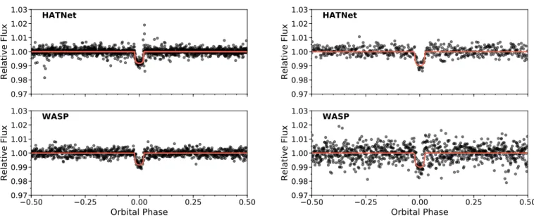
(2010). Light curves were extracted via aperture pho-tometry. Systematic effects were mitigated using Exter-nal Parameter Decorrelation (EPD,Bakos et al. 2007), and the Trend Filtering Algorithm (TFA,Kov´acs et al. 2005). Periodic transit signals were identified via the Box-fitting Least Squares analysis (BLS, Kov´acs et al. 2002). The HATNet observations are summarized in Table 1, and the discovery light curves are shown in Figure1.

2.1.2. TESS observations

HAT-P-69 and HAT-P-70 were observed by TESS during Year 1 of its primary mission. HAT-P-69 is present in the Camera 1 FFIs obtained during the Sector 7 campaign, between 2019-01-07 and 2019-02-02. HAT-P-70 is present on the Camera 1 FFIs in Sector 5, be-tween 2018-11-15 and 2018-12-11. TESS FFIs provide approximately 27 days of nearly continuous monitoring for all stars within its field of view.

We extracted the FFI light curves of the two systems with the lightkurve package (Barentsen et al. 2019) us-ing the public FFI images on MAST archive produced

from the Science Processing Operations Center (SPOC) pipeline (Jenkins et al. 2016). The raw aperture pho-tometry light curves are diluted due to the presence of nearby bright stars. In particular, HAT-P-70 is located within 3300(1.6 pixels) of a fainter star with a magnitude difference of ∆Tmag= 0.75. We extracted 10 × 10 pixel subrasters surrounding each star, and defined photomet-ric apertures to include all pixels with fluxes higher than 68% of the fluxes of nearby pixels. For HAT-P-70, this aperture includes both the target star and the nearby neighbor. For HAT-P-69, the photometric aperture does not contain any other stars within 6 magnitudes of the target star. Nearby pixels of apparently blank sky were used to estimate the background flux surrounding the target star. Figure 2 shows each star as observed by TESS, along with the photometric aperture. An R band image of the star field from the Digitized Sky Survey 2 (McLean et al. 2000) is also shown for reference. The extracted light curve of HAT-P-70 was then deblended, based on the magnitudes of nearby stars from version 6 of the TESS Input Catalog (Stassun et al. 2018).

Figures 3and4 present the TESS light curves of the target stars. The TESS light curves of HAT-P-69 and HAT-P-70 show no large systematic variation, nor signs of pulsations or additional eclipsing companions. The TESS transit signals agree in depth with the depths that are measured from ground-based observations.

Phase modulation and secondary eclipses —Hot Jupiters on circular orbits are expected to be tidally locked (e.g.

Mazeh 2008), with a fixed dayside atmosphere facing the star at all times. As a result, there can be large temperature differences between the dayside and non-illuminated nightside. During secondary eclipse, when the planet passes behind the star, the total flux from the dayside is occulted. In addition, as the planet orbits the host star, the flux from the planet’s sky-projected hemi-sphere changes periodically, producing an atmospheric brightness modulation.

To search for these signals in the TESS data, we fit a simple phase curve model to the full light curve (tran-sits, secondary eclipses, and out-of-eclipse flux modu-lation), following the methods described in detail in

Shporer et al. (2019). Given the geometry of the sys-tem, the extrema of the atmospheric brightness modu-lation occur during conjunction, i.e., a cosine of the or-bital phase. The out-of-eclipse flux is therefore given by F (t) = 1 + B1cos(φ), where φ = 2π(t − Tc) is the orbital phase, and B1 is the semi-amplitude of the phase curve signal. We include secondary eclipse signals halfway be-tween transits, with a depth parametrized by fp, i.e., the relative brightness of the planet’s dayside hemisphere.

HAT-P-69 HAT-P-70

0.97

0.98

0.99

1.00

1.01

1.02

1.03

Relative Flux

HATNet

0.50

0.25

0.00

0.25

0.50

Orbital Phase

0.97

0.98

0.99

1.00

1.01

1.02

1.03

Relative Flux

WASP

0.97

0.98

0.99

1.00

1.01

1.02

1.03

Relative Flux

HATNet

0.50

0.25

0.00

0.25

0.50

Orbital Phase

0.97

0.98

0.99

1.00

1.01

1.02

1.03

Relative Flux

WASP

Figure 1. Discovery light curves of HAT-P-69 (left) and HAT-P-70 (right). The light curves have been averaged in phase with bins of width 0.002. The top panels show the HATNet light curves, and the bottom panels show the WASP light curves.

HAT-P-69 HAT-P-70

Figure 2. Fields surrounding each of the planet-hosting stars. Top 40× 40

Digitized Sky Survey R cutouts of HAT-P-69 and HAT-P-70. Bottom TESS Full Frame Image cutouts of HAT-P-69 and HAT-P-70. The DSS and TESS cutouts are plotted at the same scale and orientation. The photo-metric apertures used to extract the TESS light curves are marked.

Since we are interested in temporal signals in the out-of-eclipse light curve, we do not use the detrended time series and instead multiply the phase curve model by generalized polynomials in time to capture all non-astrophysical time-dependent signals in the raw light

curve, which are likely attributable to instrumental sys-tematics. The raw light curves shown in Figures 3 and 4 display clear long-term temporal trends, as well as dis-continuities in flux that occur during momentum dumps. Given these discontinuities, we split each light curve into small segments separated by momentum dumps and fit a separate polynomial systematics model to each seg-ment. The orders of the polynomials used in the final fit are determined by first fitting each segment individu-ally and minimizing the Bayesian Information Criterion (BIC), defined as BIC = χ2+ k ln(n), where k is the number of fitted parameters, and n is the number of data points. After optimizing the polynomial orders, we carry out a joint fit of the full light curve.

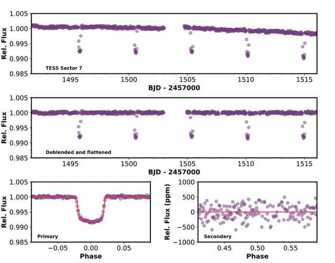
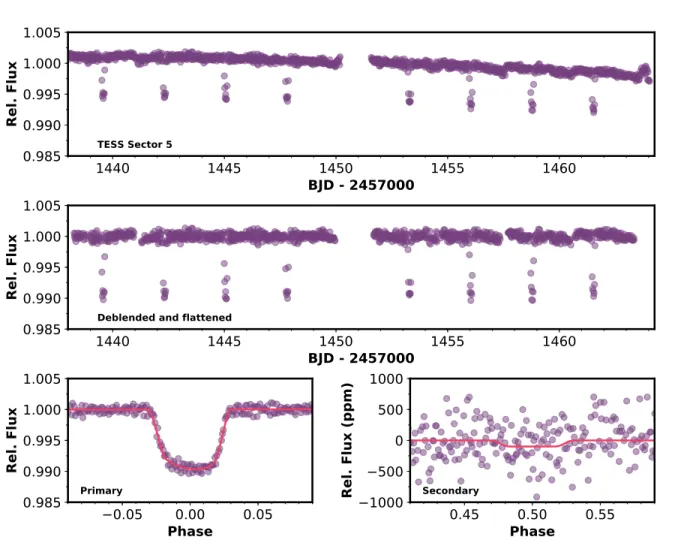
For HAT-P-70, we find that the non-astrophysical sys-tematics in the segments are well-described by poly-nomials of second to third order. In the joint fit, we report a marginal 2.4σ secondary eclipse detection of 159 ± 65 ppm, while the atmospheric brightness modu-lation amplitude is consistent with zero. Figure4shows the systematics-corrected and phase-folded light curve in the vicinity of the secondary eclipse, along with the best-fit model.

To evaluate the statistical significance of this HAT-P-70 b secondary eclipse detection, we compare the BIC of a joint fit that includes only transits and secondary eclipses (fixing B1to zero) with the BIC of a fit that as-sumes a flat out-of-transit light curve (fixing B1 and fp to zero). The difference in BIC is less than 0.1, indicat-ing that the secondary eclipse detection is not formally

1495

1500

1505

1510

1515

BJD - 2457000

0.985

0.990

0.995

1.000

1.005

Rel. Flux

TESS Sector 7

1495

1500

1505

1510

1515

BJD - 2457000

0.985

0.990

0.995

1.000

1.005

Rel. Flux

Deblended and flattened

0.05

0.00

0.05

Phase

0.985

0.990

0.995

1.000

1.005

Rel. Flux

Primary

0.45

0.50

0.55

Phase

1000

500

0

500

1000

Rel. Flux (ppm)

Secondary

Figure 3. TESS light curve of HAT-P-69. Top Raw TESS light curve. Center Detrended light curve. Lower left Detrended light curve phase folded to the transit ephemeris, showing the transit and associated best fit model (plotted in red). Lower right Detrended light curve in the region of the secondary eclipse, assuming circular orbit.

statistically robust. From an analogous analysis of the HAT-P-69 phase curve, we do not detect any significant secondary eclipse depth or phase curve signal.

2.1.3. Independent identification by WASP

HAT-P-69 and HAT-P-70 were both independently identified as planet candidates by the WASP sur-vey (Schanche et al. 2019). The northern facility (SuperWASP-North) and the southern facility (WASP-South) both consist of arrays of eight 200 mm f/1.8 Canon telephoto lenses on a common mount. Each camera is coupled with 2K × 2K detectors, yielding a field of view of 7.8 × 7.8◦ per camera (Pollacco et al. 2006). HAT-P-69 was observed by both WASP-South and SuperWASP-North, producing 25,200 photometric points spanning from 2009-01-14 to 2012-04-23. HAT-P-70 was observed by SuperWASP-North, producing 19,200 observations spanning 2008 October 13 to 2011 February 04. These long baseline observations are

plot-ted in Figure1, and were included in the global modeling (Section3.2) to help refine the transit ephemeris.

2.1.4. Ground-based follow-up observations

A series of facilities provided follow-up photometry of HAT-P-69 and HAT-P-70 to confirm the transit sig-nal, improve the determination of the the planet ra-dius, and increase the precision of the transit ephemeris. A number of transit observations were obtained with the FLWO 1.2 m telescope and KeplerCam, a 4 K × 4K CCD camera operated with 2 × 2 binning, giving a plate scale of 0.00672 pixel−1. Photometry were extracted as per Bakos et al. (2010). Follow-up photometry were also obtained using the Las Cumbres Observatory (LCO,

Brown et al. 2013) network. These observations included transits obtained via the 0.8 m LCO telescope located at the Byrne Observatory at Sedgwick, California, us-ing the SBIG STX-16803 4K × 4K camera with a field of view of 160× 160_{. Observations were also obtained}

1440

1445

1450

1455

1460

BJD - 2457000

0.985

0.990

0.995

1.000

1.005

Rel. Flux

TESS Sector 5

1440

1445

1450

1455

1460

BJD - 2457000

0.985

0.990

0.995

1.000

1.005

Rel. Flux

Deblended and flattened

0.05

0.00

0.05

Phase

0.985

0.990

0.995

1.000

1.005

Rel. Flux

Primary

0.45

0.50

0.55

Phase

1000

500

0

500

1000

Rel. Flux (ppm)

Secondary

Figure 4. TESS light curve of HAT-P-70. Panel contents as per described in Figure3. The tentative detection of a secondary eclipse, with a depth of 159 ± 65 ppm is shown in the lower right panel. The best fit model is shown in red.

using the 1 m LCO telescope at Siding Spring Observa-tory, Australia, using the Sinistro Fairchild CCD, with a field of view of 270× 270 _{over the 4K × 4K detector.} Additional photometric follow-up were obtained using the TRAPPIST (TRAnsiting Planets and PlanetesImals Small Telescope) North facility (Jehin et al. 2011;Gillon et al. 2013;Barkaoui et al. 2019) at Oukaimeden Obser-vatory in Morocco. TRAPPIST-North is a 0.6 m robotic photometer employing a 2K × 2K CCD with a field of view of 19.08 × 19.08 at a plate scale of 0.006 per pixel.

The dates, cadences, and filters used in these observa-tions are summarized in Table 1. The light curves are made available in Tables2and3, and shown in Figures5

and6.

2.2. Spectroscopy

We carried out a series of spectroscopic follow-up ob-servations to confirm the nature of the transiting can-didates, constrain the masses, and measure the orbital

obliquities of the companions. The observations are listed in Table4, and summarized below.

The Tillinghast Reflector Echelle Spectrograph (TRES,

F˝ur´esz 2008) on the 1.5 m telescope at FLWO, Arizona, was used to obtain dozens of spectra for each system. TRES is a fiber fed echelle spectrograph, with a spectral resolution of R = 44000 over the wavelength region of 3850 − 9100 ˚A. The observing strategy and data reduc-tion process are described by Buchhave et al. (2012). Each spectrum is measured from the combination of three consecutive observations for optimal cosmic ray rejection, and the wavelength solution is provided by bracketing ThAr hollow cathode lamp exposures. A series of TRES spectra were obtained at phase quadra-tures to most efficiently constrain the mass of the plan-ets. For HAT-P-69, relative radial velocities were ob-tained using a multi-order analysis (Quinn et al. 2012) of the TRES spectra. For HAT-P-70, we modeled the stellar line profiles derived from a least-squares deconvo-lution (LSD,Donati et al. 1997) to derive the absolute

Table 1. Summary of photometric observations

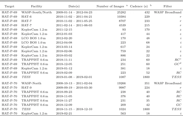
Target Facility Date(s) Number of Images a _{Cadence (s)} b _Filter

HAT-P-69 WASP-South/North 2009-01-14 – 2012-04-23 25282 432 WASP Broadband

HAT-P-69 HAT-6 2010-11-02 – 2011-04-21 10384 229 r

HAT-P-69 HAT-7 2010-11-02 – 2011-05-25 8707 233 r

HAT-P-69 HAT-7 2011-02-14 – 2011-06-03 4539 215 r

HAT-P-69 KeplerCam 1.2 m 2011-12-15 93 170 z

HAT-P-69 KeplerCam 1.2 m 2012-01-03 417 44 z

HAT-P-69 LCO BOS 1.0 m 2012-02-20 170 48 i

HAT-P-69 LCO BOS 1.0 m 2012-04-08 223 68 i

HAT-P-69 KeplerCam 1.2 m 2013-03-14 617 24 i HAT-P-69 KeplerCam 1.2 m 2018-02-06 759 22 z HAT-P-69 KeplerCam 1.2 m 2018-03-02 886 22 z HAT-P-69 TRAPPIST 0.6 m 2018-11-11 234 60 RCc HAT-P-69 TRAPPIST 0.6 m 2018-12-05 251 60 GCd HAT-P-69 KeplerCam 1.2 m 2019-01-12 381 18 i HAT-P-69 TRAPPIST 0.6 m 2019-02-09 223 52 RC

HAT-P-69 TESS 2019-01-08 – 2019-02-01 1087 1800 T ESS

HAT-P-70 WASP-North 2008-10-13 – 2011-02-04 19266 351 WASP Broadband

HAT-P-70 HAT-9 2009-09-19 – 2010-03-30 9987 224 r

HAT-P-70 TRAPPIST 0.6 m 2018-09-23 238 40 RC

HAT-P-70 TRAPPIST 0.6 m 2018-11-05 376 40 RC

HAT-P-70 TRAPPIST 0.6 m 2018-11-27 231 35 RC

HAT-P-70 TRAPPIST 0.6 m 2018-12-09 209 42 GC

HAT-P-70 TESS 2018-11-15 – 2018-12-10 1024 1800 T ESS

HAT-P-70 KeplerCam 1.2 m 2019-02-21 563 18 i

a Outlying exposures have been discarded.

b Median time difference between points in the light curve. Uniform sampling was not possible due to visibility, weather, pauses.

c RC: Red continuum filter centered at 7128 ˚A with width of 58 ˚A d GC: Green continuum filter centered at 5260 ˚A with width of 65 ˚A

Table 2. Differential photometry of HAT-P-69

BJD Mag (Raw) a _{Mag (EPD) Mag (TFA) σ Mag Instrument Filter}

2455502.9688207 9.12413 10.01248 10.00835 0.00161 HATNet r’

2455502.9733846 9.11519 10.0089 10.00331 0.0016 HATNet r’

2455502.9776452 9.11541 10.01343 10.00835 0.0016 HATNet r’

2455502.9819047 9.12139 10.01393 10.01161 0.0016 HATNet r’

2455502.9862569 9.10128 10.00651 9.99933 0.00159 HATNet r’

a This table is available in a machine-readable ascii file. A portion is shown here for guidance regarding its form and content.

Raw, EPD, and TFA magnitudes are presented for HATNet light curves. The detrending and potential blending may cause the HATNet transit to be shallower than the true transit in the EPD and TFA light curves. This is accounted for in the global modeling by the inclusion of a dilution factor. Follow-up light curves have been treated with EPD simultaneous to the transit fitting. Pre-EPD magnitudes are presented for the follow-up light curves.

Table 3. Differential photometry of HAT-P-70

BJD Mag (Raw) a Mag (EPD) Mag (TFA) σ Mag Instrument Filter

2455093.9914136 8.8238 9.69444 9.69370 0.00177 HATNet r’

2455093.9939800 8.83789 9.69611 9.70024 0.00179 HATNet r’

2455093.9966693 8.84903 9.67121 9.67967 0.0018 HATNet r’

2455093.9993076 8.80637 9.70271 9.69896 0.00177 HATNet r’

2455094.0019585 8.84992 9.69871 9.69148 0.00181 HATNet r’

a This table is available in a machine-readable form in the online journal. A portion is shown here for guidance regarding its form and content.

Raw, EPD, and TFA magnitudes are presented for HATNet light curves. The detrending and potential blending may cause the HATNet transit to be shallower than the true transit in the EPD and TFA light curves. This is accounted for in the global modeling by the inclusion of a dilution factor. Follow-up light curves have been treated with EPD simultaneous to the transit fitting. Pre-EPD magnitudes are presented for the follow-up light curves.

0.06 0.04 0.02 0.00 0.02 0.04 0.06

Orbital Phase

0.78

0.80

0.82

0.84

0.86

0.88

0.90

0.92

0.94

0.96

0.98

1.00

Relative Flux

2011 12 15

z

2012 01 03

z

2012 02 20

i

2012 04 08

i

2013 03 14

i

2018 02 06

z

2018 03 02

z

2018 11 11 RC

2018 12 05

GC

2019 01 12

i

2019 02 09 RC

Figure 5. Ground based follow-up light curves for HAT-P-69, vertically separated for clarity. The photometric band-pass and date of the observations are labeled. The facilities contributing to each light curve are presented in Table1.

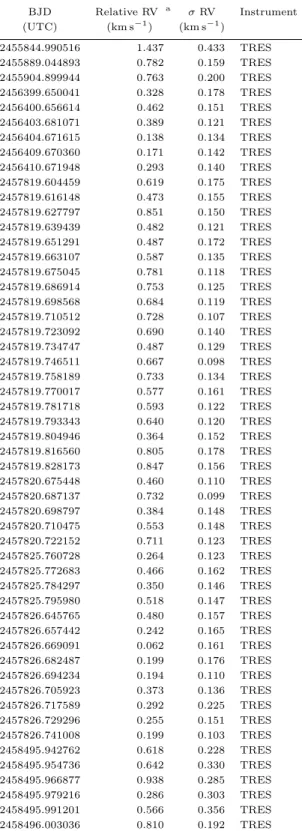
radial velocities of each spectrum. In our experience with rapidly rotating stars, the best radial velocities are obtained by modeling of the LSD-derived line profiles. The TRES velocities for HAT-P-69 and HAT-P-70 are listed in Tables5and6, and plotted in Figures7and8, respectively.

0.06 0.04 0.02 0.00 0.02 0.04 0.06

Orbital Phase

0.86

0.88

0.90

0.92

0.94

0.96

0.98

1.00

Relative Flux

2018 09 23 RC

2018 11 05 RC

2018 11 27 RC

2018 12 09

GC

2019 02 21

i

Figure 6. Ground based follow-up light curves for HAT-P-70, description as per Figure5.

Spectroscopic observations were also obtained with TRES throughout the transits of each planet. These ob-servations allow us to measure variations in the stellar line profile due to the partial obscuration of the pho-tosphere of the rapidly rotating star (Collier Cameron et al. 2010). By measuring the planetary “shadow” on the line profile of the star, we confirm that the photo-metric transit signal is indeed caused by a small body that is transiting the bright rapidly rotating target star, as opposed to being the diluted signal of a much fainter eclipsing binary that is spatially blended with the target star in the photometric aperture. The observing strat-egy and analysis largely follow the procedure laid out by

Zhou et al. (2016). We observed three partial transits of HAT-P-69 on 2017-03-08, 2017-03-13 and 2019-01-12, with the Doppler shadow of the planet clearly detected in each individual transit (Figure9). Two partial tran-sits of HAT-P-70 were obtained on 02-21 and

2019-03-04. Observations on 2019-02-21 were hampered by poor weather, but the subsequent transit on 2019-03-04 clearly revealed the planet shadow (Figure 10). These observations are used in the global analysis (Section3.2) to derive the projected spin-orbit angle of the systems.

One additional partial transit of HAT-P-69 b was obtained via the High Resolution Spectrograph (HRS

Crause et al. 2014) on the Southern African Large Tele-scope (SALT). HRS is a fiber fed echelle spectrograph, used in the medium resolution mode yielding a spec-tral resolution of R = 40000 over the wavelength region of 3700 − 5500 ˚A over the blue arm of the spectrograph. Observations from the red arm of the spectrograph were not used due to the fewer line-count over its spectral coverage. The observations were obtained covering the ingress of HAT-P-69 b on 2015-03-06, covering 11 spec-tra with integration times of 700 s each. The target star remained at an altitude of 47 − 53◦throughout the tran-sit observations. The spectra were extracted and cali-brated using the MIDAS pipeline (Kniazev et al. 2016,

2017). The spectral line profiles were extracted via a similar process as that described above. The average line profile is subtracted, leaving a significant detection of the planetary transit over ingress (Figure9).

In addition, a number of spectroscopic resources con-tributed to the initial spectroscopic vetting of the tar-gets. Observations of HAT-P-69 were obtained using the High Resolution Echelle Spectrometer (HIRES) on the 10 m Keck-I at Mauna Kea Observatory. Obser-vations were also obtained using the High Dispersion Spectrograph (HDS) on the 8.2 m Subaru telescope on Mauna Kea Observatory. In both cases observations were made using the Iodine cell, but did not yield high precision velocities due to the rapid rotation of the star. They were not included in the analysis. We also made use of the CHIRON instrument on the SMARTS 1.5 m telescope at Cerro Tololo Inter-American Observatory (CTIO), Chile (Tokovinin et al. 2013), obtaining 4 servations of HAT-P-70. Similarly, reconnaissance ob-servations were obtained with the SOPHIE echelle facil-ity on the 1.93 m Haute-Provence Observatory, France, as well as the CORALIE spectrograph on the 1.2 m Eu-ler telescope at the ESO La Silla Observatory, Chile. Given that the TRES observations vastly outnumber these reconnaissance observations, we incorporate only the TRES data in our global modeling.

3. ANALYSIS

3.1. Properties of the host star

Both HAT-P-69 and HAT-P-70 are classified as rapidly rotating A stars based on their 2MASS ( Skrut-skie et al. 2006) J − K colors and the reconnaissance

0.00

0.25

0.50

0.75

1.00

Orbital Phase

1000

750

500

250

0

250

500

750

1000

RV

(m

s

)

TRES

Figure 7. TRES radial velocities for HAT-P-69. The best fit orbit from the global model is plotted in red. The fitted radial velocity jitter has been added to the per-point uncertainties in quadrature.

0.00

0.25

0.50

0.75

1.00

Orbital Phase

3000

2000

1000

0

1000

2000

3000

RV

(m

s

)

TRES

Figure 8. TRES radial velocities for HAT-P-70, caption as per Figure7.

spectra from TRES. Rapidly rotating stars have spectral lines that are blended and unresolved, making standard spectral classifications more difficult. In addition, the gravity darkening effect causes the derived atmospheric parameters, such as effective temperature, to be depen-dent on our viewing angle. The same star would appear hotter when viewed pole-on, and cooler when viewed along the equator. We adopt the approach described in

Zhou et al.(2019) and match the spectral energy distri-bution of the star against a grid of synthetic magnitudes computed from the Geneva 2D rotational isochrones

Table 4. Summary of spectroscopic observations

Target Telescope/Instrument Date Range Number of Observations Resolution Observing Mode

HAT-P-69 FLWO 1.5 m TRES 2011-10-10 – 2017-03-14 45 44000 RV

HAT-P-69 SALT HRS 2015-03-06 11 40000 Transit

HAT-P-69 FLWO 1.5 m TRES 2017-03-08 18 44000 Transit

HAT-P-69 FLWO 1.5 m TRES 2017-03-13 17 44000 Transit

HAT-P-69 FLWO 1.5 m TRES 2019-01-12 22 44000 Transit

HAT-P-70 FLWO 1.5 m TRES 2013-02-01 – 2019-02-20 43 44000 RV

HAT-P-70 FLWO 1.5 m TRES 2019-02-21 19 44000 Transit

HAT-P-70 FLWO 1.5 m TRES 2019-03-04 19 44000 Transit

HAT-P-69

Orbital Phase

Model

Ingress

Egress

vs

ini

vs

ini

Velocity(kms

₎

Residuals

Orbital Phase

Model

Ingress

Egress

vs

ini

vs

ini

Velocity(kms

₎

Residuals

Figure 9. The Doppler transits of HAT-P-69 b. Each Doppler map (top panel) shows the intensity of the line profile as a function of both velocity (relative to the line center) and orbital phase. The ingress and egress phases are marked with horizontal lines. The top segment shows the data from all the observed transits, averaged into phase bins of size 0.003. The middle panel shows the best-fitting model, and the lower panel shows the residuals. A diagrammatic representation of the transit geometry of each system is shown at the top of the figure, with the relative sizes of the star and planet plotted to scale. The gravity darkening effect is exaggerated to allow it to be easily seen. The left panel shows the Doppler transit signal for HAT-P-69 b, combined from 3 partial TRES transit observations. The right panels shows the partial transit of HAT-P-69 b via SALT-HRS. Phases at which no data was obtained are colored in plain orange.

Table 5. Relative radial velocities of HAT-P-69 BJD Relative RV a _{σ RV Instrument} (UTC) (km s−1_{) (km s}−1₎ 2455844.990516 1.437 0.433 TRES 2455889.044893 0.782 0.159 TRES 2455904.899944 0.763 0.200 TRES 2456399.650041 0.328 0.178 TRES 2456400.656614 0.462 0.151 TRES 2456403.681071 0.389 0.121 TRES 2456404.671615 0.138 0.134 TRES 2456409.670360 0.171 0.142 TRES 2456410.671948 0.293 0.140 TRES 2457819.604459 0.619 0.175 TRES 2457819.616148 0.473 0.155 TRES 2457819.627797 0.851 0.150 TRES 2457819.639439 0.482 0.121 TRES 2457819.651291 0.487 0.172 TRES 2457819.663107 0.587 0.135 TRES 2457819.675045 0.781 0.118 TRES 2457819.686914 0.753 0.125 TRES 2457819.698568 0.684 0.119 TRES 2457819.710512 0.728 0.107 TRES 2457819.723092 0.690 0.140 TRES 2457819.734747 0.487 0.129 TRES 2457819.746511 0.667 0.098 TRES 2457819.758189 0.733 0.134 TRES 2457819.770017 0.577 0.161 TRES 2457819.781718 0.593 0.122 TRES 2457819.793343 0.640 0.120 TRES 2457819.804946 0.364 0.152 TRES 2457819.816560 0.805 0.178 TRES 2457819.828173 0.847 0.156 TRES 2457820.675448 0.460 0.110 TRES 2457820.687137 0.732 0.099 TRES 2457820.698797 0.384 0.148 TRES 2457820.710475 0.553 0.148 TRES 2457820.722152 0.711 0.123 TRES 2457825.760728 0.264 0.123 TRES 2457825.772683 0.466 0.162 TRES 2457825.784297 0.350 0.146 TRES 2457825.795980 0.518 0.147 TRES 2457826.645765 0.480 0.157 TRES 2457826.657442 0.242 0.165 TRES 2457826.669091 0.062 0.161 TRES 2457826.682487 0.199 0.176 TRES 2457826.694234 0.194 0.110 TRES 2457826.705923 0.373 0.136 TRES 2457826.717589 0.292 0.225 TRES 2457826.729296 0.255 0.151 TRES 2457826.741008 0.199 0.103 TRES 2458495.942762 0.618 0.228 TRES 2458495.954736 0.642 0.330 TRES 2458495.966877 0.938 0.285 TRES 2458495.979216 0.286 0.303 TRES 2458495.991201 0.566 0.356 TRES 2458496.003036 0.810 0.192 TRES

a Relative radial velocities from a multi-order cross correla-tion. Internal errors excluding the component of astrophys-ical/instrumental jitter considered in Section 3. Velocities exclude those taken in transit.

Table 6. Relative radial velocities of HAT-P-70.

BJD RV a σ RV Instrument (UTC) (km s−1) (km s−1) 2456324.697671 24.350 0.642 TRES 2456342.685872 24.867 0.616 TRES 2457671.822407 25.153 0.708 TRES 2457671.830590 25.270 0.620 TRES 2457671.838751 26.999 0.532 TRES 2457671.846928 25.516 0.639 TRES 2457671.855187 25.525 0.727 TRES 2457671.863348 25.804 1.043 TRES 2457671.871531 25.827 0.599 TRES 2457671.880432 26.936 0.676 TRES 2457671.892204 24.786 1.114 TRES 2457671.900399 24.601 0.688 TRES 2457671.908554 24.334 0.934 TRES 2457671.917565 24.760 0.634 TRES 2457671.925743 25.362 0.773 TRES 2457671.933920 24.981 0.663 TRES 2457671.942121 25.324 0.659 TRES 2457671.950363 26.011 0.538 TRES 2457671.958645 25.100 0.825 TRES 2457671.966979 25.709 0.726 TRES 2457671.975226 24.904 0.592 TRES 2457671.983427 25.817 0.819 TRES 2457671.991639 24.845 0.677 TRES 2457672.000309 25.261 0.536 TRES 2457672.008573 24.851 0.584 TRES 2457672.016844 25.661 0.839 TRES 2457672.025149 25.769 0.434 TRES 2458527.601110 25.803 1.160 TRES 2458531.776169 25.321 1.741 TRES 2458532.755301 24.806 0.962 TRES 2458534.591655 24.475 0.630 TRES 2458534.599808 25.870 0.654 TRES 2458534.607915 25.156 1.032 TRES 2458534.616045 24.988 0.569 TRES 2458534.624158 25.590 0.992 TRES 2458534.632322 24.981 0.916 TRES 2458534.640470 26.307 1.199 TRES 2458534.648681 24.680 0.628 TRES 2458534.656811 25.248 1.155 TRES 2458534.664964 24.315 0.761 TRES 2458534.673094 25.971 0.920 TRES 2458534.681230 24.672 0.470 TRES 2458534.689354 24.547 0.848 TRES 2458535.714170 24.300 0.508 TRES 2458535.722375 23.870 0.994 TRES 2458535.730499 24.905 2.141 TRES 2458535.738629 23.029 3.309 TRES 2458546.689854 25.441 0.382 TRES 2458546.698076 26.287 0.618 TRES 2458546.706287 24.819 0.922 TRES 2458546.714516 26.252 0.741 TRES 2458546.722686 23.979 0.821 TRES 2458546.730914 25.292 1.133 TRES 2458546.739183 25.804 1.377 TRES a Absolute velocities from derived from the least-squares

deconvolution profiles. Internal errors excluding the component of astrophysical/instrumental jitter consid-ered in Section 3. Velocities exclude those taken in transit.

HAT-P-70

Orbital Phase

Model

Ingress

Egress

vs

ini

vs

ini

Velocity(kms

₎

Residuals

Figure 10. The Doppler transit HAT-P-70 b as measured via two partial TRES transits. The figure follows the format specified in Figure9.

(Ekstr¨om et al. 2012) for a range of inclination angles. This is performed as part of the global modeling de-scribed in Section 3.2, as the transit light curve also contributes to constraining the inclination angle of the system.

The spectral energy distributions (SED) for both stars are shown in Figures 11 and 12. We find that both stars are late A dwarfs. HAT-P-69 has a mass of 1.648+0.058_−0.026M, radius of 1.926+0.060−0.031R, and effective temperature of 7394+360₋₆₀₀K. HAT-P-70 has a mass of 1.890+0.010_−0.013M, radius of 1.858+0.119−0.091R, and effective temperature of 8450+540₋₆₉₀K.

We check this rotational-SED analysis with an inde-pendent fit of the SEDs to Kurucz atmosphere models of non-rotating stars (Kurucz 1992). We find HAT-P-69 to have Teff = 7650 ± 400 K, R? = 1.88 ± 0.19 R, and reddening of A(v) = 0.01 ± 0.01. While HAT-P-70 has Teff = 8400 ± 400 K, R? = 2.08 ± 0.20 R, with

reddening of A(v) = 0.30+0.01_−0.08. For both stars, the non-rotational SED analysis agrees well with that from the global modeling detailed above.

As a check on the determination of the stellar pa-rameters, we independently derived the effective tem-perature and metallicity of each star using the TRES spectra and the Stellar Parameter Classification (SPC) pipeline (Buchhave et al. 2010). We find HAT-P-69 to have Teff = 7557 ± 52 K, [m/H] = +0.05 ± 0.08 dex, while HAT-P-70 has atmospheric parameters of Teff = 8246 ± 93 K and [m/H] = −0.06 ± 0.09 dex. The spectroscopic stellar parameters agree to within 1σ with those measured from the SED, though the uncertain-ties are likely underestimated. The rapid rotation of the star causes difficulties in continuum normalization of the spectra, making accurate spectroscopic determination of the stellar parameters and associated uncertainties more difficult. We incorporate the metallicity measurements from spectra as Gaussian priors in the global modeling. For a more accurate understanding of stellar properties, we simulataneously fit the SED with the transit and rotational stellar isochrones in our global modeling, in-stead of relying on the spectra-derived values.

An accurate measurement of the projected stellar ro-tation rate is crucial for interpreting the Doppler tran-sit data, constraining the stellar gravity darkening ef-fect, and constraining the stellar oblateness. To mea-sure the projected rotation velocity, we model the LSD spectral line profiles using a kernel that incorporates the effects of stellar rotation and radial-tangential macro-turbulence via a numerical disk integration, and the models the instrument line broadening as a Gaussian convolution. We find HAT-P-69 to have v sin I? = 77.40 ± 0.60 km s−1 and a macroturbulent velocity of vmac = 5.6 ± 4.2 km s−1. For HAT-P-70, the results are v sin I? = 99.87 ± 0.65 km s−1 and vmac = 4.77 ± 0.86 km s−1.

3.2. Global modeling of system parameters We perform a global analysis of the systems to model the large suite of observations available for HAT-P-69 and HAT-P-70. This global model simultaneously incor-porates the photometric transit, radial velocities, stellar parameter constraints, the Doppler transits, and the ef-fect of photometric gravity darkening on the transit light curve and observed stellar properties.

Our modeling process largely follows that described by

Zhou et al. (2019). Rapid rotation distorts the shapes of stars; they become oblate along the equator, causing the poles to be hotter and brighter, while the equator becomes cooler and darker (von Zeipel 1924). This grav-ity darkening effect causes both the transit light curve

3000

10000

30000

Wavelength

(

Å

)

1.0

0.1

λF

(

λ

)

(N

or

m

ali

ze

d)

Figure 11. Spectral energy distribution of HAT-P-69 with the B, V , g0, r0, and i0 bands from APASS (Henden et al. 2016), G, BP, and RP from Gaia (Gaia Collaboration et al.

2018), and J , H, Ks from 2MASS (Skrutskie et al. 2006). The synthetic spectrum is generated using ATLAS9 models (Castelli & Kurucz 2004) whilst accounting for the effect of the viewing geometry and gravity darkening of the host star.

3000

10000

30000

Wavelength

(

Å

)

1.0

0.1

λF

(

λ

)

(N

or

m

ali

ze

d)

Figure 12. Spectral energy distribution of HAT-P-70, similar to Figure11. See caption for Figure11.

(Barnes 2009) and the observed spectral energy distri-bution of the star (Brandt & Huang 2015) to depend on the viewing direction. The photometric transit is mod-eled using the simuTrans package from Herman et al.

(2018), which accounts for both the gravity darkened non-uniform brightness distribution of the stellar disk, and the ellipsoidal nature of the rapidly rotating star. The stellar properties are inferred from the Geneva 2D rotational isochrones (Ekstr¨om et al. 2012), which in-corporates the effects of rotation on stellar evolution, and includes prescriptions for the oblateness of the stars based on their rotation rates. In the case of an oblique transiting geometry about gravity darkened stars, the

resulting light curve often exhibits asymmetry due to the latidude dependence of the surface brightness dis-tribution. This effect is detected for HAT-P-70 b, and explored in greater depth in Section3.4.

The limb darkening coefficients are interpolated from the values ofClaret & Bloemen(2011) andClaret(2017) for the Sloan and TESS bands. They are constrained by a Gaussian prior of width 0.02 during the global model-ing, representing the difference in the limb darkening coefficients should the stellar parameters be different by 1σ. To model the transit light curves, we adopt a gravity darkening coefficient β from interferometric ob-servations of Vega (β = 0.231 ± 0.028) (Monnier et al. 2012). Similar interferometric gravity darkening coeffi-cients have been measured for other rapidly rotating A stars (e.g. α Cep β = 0.216 ± 0.021 Zhao et al. 2009). To account for the uncertainty in the gravity darken-ing coefficient, it is modeled in the global fit as a free parameter constrained about the value and uncertainty of Vega reported in Monnier et al. (2012). The model fitting procedure also includes detrending of the ground-based follow-up light curves, via a linear combination of effects, including the pixel position of the target star, airmass, and background count values. We account for the 30 minute cadence of the TESS by super-sampling and integrating the model over the exposure time.

The stellar parameters are constrained by the spectral energy distribution of the stars over the Tycho-2 (Høg et al. 2000), APASS (Henden et al. 2016), and 2MASS (Skrutskie et al. 2006) photometric bands, as well as the parallax from Gaia data release 2 (Gaia Collaboration et al. 2018). Local reddening is constrained by the max-imum reddening value from the dust maps of Schlafly & Finkbeiner(2011), assuming Av = 3.1E(B − V ). To account for the uncertainties in our deblending of the TESS light curves, we also include a TESS light curve dilution parameter, closely constrained by a Gaussian prior, with width derived from the reported uncertain-ties in the TESS band magnitudes of the target and nearby stars from TIC v6.

The Doppler transit signal is simultaneously modeled with the light curve, and provides the best constraint on the projected spin-orbit angle λ for the orbital plane of the planets. We model variations of the stellar line profiles via a 2D integration of the rotating stellar sur-face being occulted by the transiting planet, incorpo-rating the effects of differential limb darkening, radial-tangential macroturbulence, and instrument broaden-ing.

To derive the best fit system parameters and their associated uncertainties, we perform a Markov Chain Monte Carlo analysis using the emcee package (

Foreman-Mackey et al. 2013). The resulting stellar and planetary parameters are shown in Tables7 and8, respectively.

3.3. Blending and astrophysical false positive scenarios Many astrophysical scenarios can mimic the tran-sit signal of a planetary system. False positive sce-narios such as M-dwarf companions with similar radii as substellar counterparts are ruled out by the mass constraints imposed by our radial velocity measure-ments. The possibility that the transit signals are due to fainter eclipsing binaries whose eclipses are diluted by the brighter target stars are more difficult to elim-inate. We adopt a number of observations, including diffraction-limited imaging, and analysis of the spectro-scopic transit, to eliminate this possibility.

To rule out spatially nearby companions, we ob-tained observations with the NN-explore Exoplanet Stel-lar Speckle Imager (NESSI, Scott et al. 2018) on the 3.5 m WIYN telescope at Kitt Peak National Observa-tory, Arizona, USA. Speckle imaging gives a resolution of &0.0400 in both the r-narrow and z-narrow bands for both HAT-P-69 and HAT-P-70, corresponding to spa-tial scales as close to the stars as 14 to 22 AU (at 562 nm and 832 nm respectively). The corresponding constraints from NESSI are plotted in Figure13. In ad-dition, we obtained J and Ks band infrared seeing lim-ited imaging HAT-P-69 with the WIYN High-Resolution Infrared Camera (WHIRC,Smee et al. 2011), also find-ing no visual companions to the target star.

Finally, the Doppler detection of the planetary tran-sit confirms that the trantran-sits indeed occur around the rapidly rotating bright A star hosts, not background stars (e.g.Collier Cameron et al. 2010). The depth of the spectroscopic shadow agrees with the depth observed in the photometric light curves, suggesting that the dilu-tion due to background sources is negligible.

3.4. Detection of an asymmetric gravity darkened transit for HAT-P-70

A transiting planet crossing a gravity darkened stel-lar disk may exhibit an asymmetric transit when the projected spin-orbit angle is misaligned with the stel-lar rotation axis. The effects specific to gravity dark-ening are only visible at the parts-per-thousand level, and as such they are difficult to detect with ground-based data. The only previous confirmed instance of asymmetric gravity darkening being observed for a plan-etary system is for Kepler-13. The asymmetric transit light curves of Kepler-13 were identified and modeled by

Szab´o et al. (2011), Barnes et al. (2011), and Herman et al. (2018). Subsequent ground-based Doppler tran-sit confirmation of the spin-orbit misalignment was per-formed byJohnson et al.(2014), and an eventual joint

light curve and spectroscopic transit model developed byMasuda(2015).

The TESS light curves of HAT-P-70 exhibit asym-metric transits similar to those seen for Kepler-13. The transit is shallower at ingress, and deeper near egress, in-dicating that the planet traverses a stellar surface that is darker near ingress, and brighter near egress. Our global model reproduces such a transit, with the pro-jected spin-orbit misaligned at 21.2+4.6_−3.6◦, and the stellar pole inclined to the line of sight by 58.2+1.6_−1.2◦ degrees. Figure14shows the TESS transit light curve, with the best fit standard and gravity-darkened transit models over-plotted. An asymmetry at the 500 ppm level can be seen in the residuals to the standard transit model, akin to that seen for Kepler-13.

We note that we make use of the bolometric gravity darkening coefficient β in our light curve modeling. Im-provements can be made via a more careful treatment for the band-dependence of the gravity darkening effect (e.g.Espinosa Lara & Rieutord 2011). We note though that running the global modeling whilst allowing β to be free re-produces the same projected obliquity λ value to within uncertainties, and as such the actual adopted gravity darkening coefficient is not critical to the mod-eling.

4. THE OCCURRENCE RATE OF HOT JUPITERS

FROM TESS

Although hot Jupiters were some of the earliest exo-planets to be discovered, they are not intrinsically com-mon. Radial velocity searches from the Keck, Lick, and Anglo Australia Telescope programs of 1,330 FGK stars revealed a hot Jupiter occurrence rate of 1.2 ± 0.2% (< 15 MJup, < 0.1 AU Marcy et al. 2005), revised to 1.20 ± 0.38% (> 0.1 MJup, P < 10 days) by Wright et al. (2012) using the California Planet Search sam-ple. Cumming et al.(2008) found an occurrence rate of 1.5±0.6% (> 0.3 MJup, < 0.1 AU) using the Keck planet search sample. Using the HARPS and CORALIE sam-ple,Mayor et al.(2011) found a hot Jupiter occurrence rate of 0.89 ± 0.36% (> 0.15 MJup, < 11 days).

These radial velocity occurrence rates are generally thought to be higher than those offered by the Kepler survey. Studies byHoward et al.(2012) andFressin et al.

(2013) of the early Kepler data found rates of 0.4 ± 0.1% and 0.43 ± 0.05% for hot Jupiters respectively. Recent analyses with improved stellar properties fromPetigura et al. (2018) found that 0.57+0.14_−0.12% of main sequence FGK stars (5.0 > log g > 3.9, 4200 < Teff < 6500 K) host hot Jupiters. The measured giant planet occur-rence rate from the CoRoT mission is higher than that from Kepler, finding 21 giant planets (Rp > 5 R⊕)

Table 7. Stellar parameters

Parameter HAT-P-69 HAT-P-70

Catalogue Information TIC . . . 379929661 399870368 Tycho-2 . . . 0215-01594-1 0688-01684-1 Gaia DR2 . . . 3080104185367102592 3291455819447952768 Gaia RA (2015.5) . . . 08:42:01.353 04:58:12.560 Gaia DEC (2015.5) . . . +03:42:38.038 +09:59:52.726 Gaia µα(mas yr−1) . . . −2.856 ± 0.074 −2.657 ± 0.096 Gaia µδ(mas yr−1) . . . 0.984 ± 0.051 −4.996 ± 0.065

Gaia DR2 Parallax (mas) . . 2.902 ± 0.043 2.996 ± 0.061 Stellar atmospheric propertiesa

Teff?(K) . . . 7394+360−600 8450 +540 −690 [Fe/H] . . . −0.069+0.058−0.075 −0.059 +0.075 −0.088 v sin I?(km s−1) . . . 77.44+0.55−0.57 99.85 +0.64 −0.61 vmacro(km s−1) . . . 5.76+0.24−0.24 5.870 +0.58 −0.52 Photometric properties TESS T (mag) . . . 9.612 ± 0.018 9.298 ± 0.019 Gaia G (mag) . . . 9.77216 ± 0.00035 9.45112 ± 0.00035 TYCHO B (mag) . . . 10.052 ± 0.061 9.621 ± 0.045 TYCHO V (mag) . . . 9.7740 ± 0.0050 9.4700 ± 0.0040 APASS g0(mag) . . . 9.796 ± 0.030 9.842 ± 0.351 APASS r0(mag) . . . 9.855 ± 0.041 9.506 ± 0.028 APASS i0(mag) . . . 9.976 ± 0.020 9.962 ± 0.061 2MASS J (mag) . . . 9.373 ± 0.024 9.068 ± 0.022 2MASS H (mag) . . . 9.293 ± 0.022 9.023 ± 0.029 2MASS Ks(mag) . . . 9.280 ± 0.023 8.963 ± 0.024 Stellar properties M?(M) . . . 1.648+0.058−0.026 1.890 +0.010 −0.013 R?(R) . . . 1.926+0.060−0.031 1.858 +0.119 −0.091 log g?(cgs) . . . 4.110+0.034−0.064 4.181 +0.055 −0.063 L?(L) . . . 10.0+1.8−0.9 16.7 +5.3 −4.6

Stellar oblateness Rpole/Req 0.9678+0.0012−0.0022 0.9574 +0.0063 −0.0057

Line of sight inclination I∗. . 58.2+1.6−1.2 58.8+7.5−4.8

E(B − V ) (mag)b_{. . . . 0.0167}+0.011 −0.015 < 0.034 (1σ) Age (Gyr) . . . 1.27+0.28 −0.44 0.60+0.38−0.20 Distance (pc) . . . 343.9+4.8 −4.3 329.0 ± 6.5

a Derived from the global modeling described in Section 3, co-constrained by spectroscopic stellar parameters and the Gaia DR2 parallax.

b Uniform prior for reddening up to the local maximum set bySchlafly & Finkbeiner (2011)

within 10 day period orbits, corresponding to an oc-currence rate of 0.98 ± 0.26 % (Deleuil et al. 2018).

The stars that host hot Jupiters are more metal rich than random stars of the same spectral class (Petigura et al. 2018; Santos et al. 2003; Valenti & Fischer 2005;

Buchhave et al. 2012). Differences between the metallic-ity distribution of the Kepler stellar sample and those of the radial velocity surveys have been raised as an explanation for the differenes in the hot Jupiter occur-rence rates (Wright et al. 2012), although Guo et al.

(2017) showed that there is minimal difference between the Kepler field star metallicity distribution and that of the California Planet Search sample. Wang et al.(2015) offered a correction for the Kepler sample based on an improved classification of the subgiant population. They suggested that multiplicity or a lower occurrence rate of hot Jupiters around sub giants may be the cause of the disagreement. Later,Bouma et al. (2018) showed that binarity is unlikely to be responsible for any disagree-ments between the Doppler and Kepler samples.

Table 8. Orbital and planetary parameters

Parameter HAT-P-69 b HAT-P-70 b

Light curve parameters

P (days) . . . 4.7869491+0.0000018_−0.0000021 2.74432452+0.00000079_{−0.00000068} Tc(BJD − TDB)a . . . 2458495.78861+0.00072−0.00073 2458439.57519 +0.00045 −0.00037 T14(days)a . . . 0.2136+0.0014−0.0014 0.1450 +0.0028 −0.0020 a/R? . . . 7.32+0.16−0.18 5.45 +0.29 −0.49 Rp/R? . . . 0.08703+0.00075−0.00080 0.09887 +0.00133 −0.00095 b ≡ a cos i/R? . . . 0.366+0.060−0.050 −0.629 +0.081 −0.054 i (deg) . . . 87.19+0.52_−0.72 96.50+1.42_−0.91 |λ| (deg) . . . 21.2+4.6_−3.6 113.1+5.1_−3.4

Limb-darkening and gravity darkening coefficientsb

a0_r(HAT) (linear term) . . . 0.1194 (fixed) 0.1550 (fixed) b0_r(HAT) (quadratic term) . . . 0.3974 (fixed) 0.3306 (fixed) aGC . . . 0.41+0.09−0.10 0.43 +0.10 −0.10 bGC . . . 0.25+0.09−0.11 0.25 +0.09 −0.11 aRc . . . 0.30+0.10−0.09 0.24 +0.10 −0.09 bRc . . . 0.21+0.10−0.11 0.19 +0.10 −0.10 a0_i . . . 0.117+0.018 −0.018 0.239+0.018−0.021 b0_i . . . 0.392+0.020 −0.019 0.338+0.021−0.020 a0_z . . . 0.069+0.018 −0.018 b0_z . . . 0.389+0.020 −0.020 aTESS . . . 0.238+0.021−0.019 0.149+0.018−0.021 bTESS . . . 0.286+0.015−0.019 0.313+0.019−0.022

β Gravity darkening coefficient . . . 0.239+0.026

−0.029 0.242+0.026−0.029 RV parameters K (m s−1) . . . 309+49₋₄₉ < 649 (3σ) e . . . 0 (fixed) 0 (fixed) RV jitter (m s−1) . . . 53+34₋₃₇ 320+180₋₁₈₀ Systemic RV (m s−1)c . . . 784 ± 24 25260 ± 110 Planetary parameters Mp(MJ) . . . 3.58+0.58−0.58 < 6.78 (3σ) Rp(RJ) . . . 1.676+0.051−0.033 1.87 +0.15 −0.10 ρp(g cm−3) . . . 1.02+0.18−0.16 < 1.54 (3σ) log gp(cgs) . . . 3.521+0.067−0.071 < 3.73 (3σ) a (AU) . . . 0.06555+0.00070_−0.00035 .04739+0.00031_−0.00106 Teq(K)d . . . 1930+80−230 2562 +43 −52

a Tc: Reference epoch of mid transit that minimizes the correlation with the orbital period. T14: total

transit duration, time between first to last contact;

b Values for a quadratic law given separately for each of the filters with which photometric observations were obtained. These values were adopted from the tabulations byClaret & Bloemen(2011) according to the spectroscopic an initial estimate of the stellar parameters. The limb darkening coefficients are constrained by strong Gaussian priors of width 0.02 about their initial values. The Gravity darkening coefficient β is also constrained by a Gaussian prior of width 0.028 in the fit.

c The systemic RV for the system as measured relative to the telluric lines d Teqcalculated assuming 0 albedo and full heat redistribution

HAT-P-69 HAT-P-70

NESSI Blue (562 nm)

1"

NESSI Red (832 nm)

1"

0.0

0.5

1.0

1.5

2.0

2.5

Separation (arcsec)

0

2

4

6

8

Ma

g

NESSI Blue (562 nm)

1"

NESSI Red (832 nm)

1"

0.0

0.5

1.0

1.5

2.0

2.5

Separation (arcsec)

0

2

4

6

8

Ma

g

Figure 13. Images and constraints on spatially separated stellar companions via speckle imaging for HAT-P-69 and HAT-P-70 from NESSI. Companions with separations & 0.0400are ruled out. The blue and orange lines mark the 5σ limit on the detection of companions via the blue and red NESSI cameras.

0.990 0.992 0.994 0.996 0.998 1.000 1.002

Relative Flux

Gravity Darkened Model

0.002 0.000 0.002

Residual

0.05 0.00 0.05

Orbital Phase

0.002 0.000 0.002

Residual

Figure 14. The TESS transit light curve of HAT-P-70. Note that the transit is asymmetric, being shallower near ingress, and deeper near egress. This is due to the planet traversing from the gravity darkened equator to brighter pole during the transit. The middle panel shows the light curve residual of a standard, symmetric transit model. There are systematic variations in the residuals due to the gravity dark-ening effect. The bottom panel shows the residuals when the best fit gravity darkening model is subtracted.

A radial velocity survey of intermediate-mass sub-giants has shown that higher mass stars tend to host more gas giant planets within a few AU (e.g. Johnson et al. 2010;Jones et al. 2014;Reffert et al. 2015;Ghezzi et al. 2018), though caveats regarding the accuracy of the mass measurements of these evolved stars should be noted (e.g. Lloyd 2013; Schlaufman & Winn 2013;

Stello et al. 2017). The giant planets around subgiants tend to be found in orbits beyond 0.1 AU; there appears to be a paucity of hot Jupiters around evolved stars. These studies suggest that hot Jupiters undergo tidal orbital decay when a star begins evolving into a sub-giant (Schlaufman & Winn 2013). The planets around these “retired A stars” tend to be in longer period, more circular orbits than those found around main sequence stars (Jones et al. 2014) — although recent discoveries have unveiled numerous hot Jupiters in close-in orbits about evolved stars (Grunblatt et al. 2018). These is-sues inspired us to look into the hot Jupiter occurrence rate around main-sequence A stars.

In this section, we aim to examine the hot Jupiter occurrence rate via the TESS stellar population, with two key differences to the previous works from Kepler.

• The TESS stellar population encompasses bright stars covering a quarter of the sky. This sample is a significantly closer (150 pc for a Solar-type main-sequence star) population than that from Kepler. The TESS sample is a closer match to the radial velocity sample of bright nearby stars, and should provide another test for any tension in the occur-rence rates derived by the two techniques.

• The TESS sample spans A, F, and G main se-quence stars. By comparing the planet distribu-tion around A and FG samples, we can determine if the paucity of close-in planets around “retired A stars” is due to post-main-sequence stellar evo-lution. More broadly, we can test whether the oc-currence rates of hot Jupiters changes with stellar mass.

4.1. Main-sequence sample

We restricted our study to main-sequence stars. We did not wish to consider evolved stars because of the problems with selection biases, shallower transit depths, and lack of substantial follow-up observations. We do note, though, that more than half of the TESS stars brighter than 10th magnitude are evolved. Eventually, this will be a rich hunting ground (e.g.Huber et al. 2019;

Rodriguez et al. 2019).

Figure 15 shows the colour-magnitude diagram (CMD) of the 120,000 stars brighter than Tmag = 10 that were observed by TESS. The BP − RP and G values are taken from a cross match against the Gaia DR2 catalogue (Gaia Collaboration et al. 2018). To define the main sequence, we make use of the colors and magnitudes from the MESA Isochrones and Stel-lar Tracks (MIST) (Dotter 2016). We draw an upper and a lower boundary in the BP − RP vs G diagram based on the Zero Age Main Sequence (ZAMS) and the Terminal Age Main Sequence (TAMS) points in the solar metallicity MIST evolution tracks. As perDotter

(2016), the ZAMS is defined by the criterion that the core hydrogen luminosity of the star is 99.9% that of the total core luminosity, while the TAMS is defined by the criterion that the core hydrogen fraction has fallen below 10−12. The ZAMS and TAMS boundaries are plotted in Figure15. Between these boundaries, we are left with 47,126 main sequence stars for this study.

The restriction to stars with Tmag < 10 allows us to make use of the TOI catalogue available to the TESS follow-up community, which is essentially complete for

0.5

0.0

0.5

1.0

1.5

2.0

B

P

R

P

(mag)

4

2

0

2

4

6

8

10

G

(m

ag

)

HAT-P-70

_HAT-P-69

0.4

M

1.0

M

2.0

M

3.0

M

Confirmed Planet

Candidate

Figure 15. The Gaia CMD for stars brighter than Tmag= 10 observed within the first seven sectors of the TESS mission. The Zero Age Main Sequence (lower) and Terminal Age Main Sequence (upper) boundaries are plotted to mark the main sequence. Evolution tracks from the MIST isochrones (Dotter 2016) spaced at 0.2 M intervals are plotted across the main sequence. Close in giant planets discovered or recovered by TESS are plotted, marked in solid stars for confirmed planets, and open circles for planet candidates. Planet candidates off the main sequence, or around cool stars, but in the TESS Objects of Interest are are plotted on this diagram for completeness, but not included in the analysis.

hot Jupiters. The planet candidates around fainter stars in the FFIs are not fully vetted. We also restrict atten-tion to the data from Sectors 1-7 because the candidates derived from later Sectors have not yet received sufficient follow-up observations at the time of writing.

To check our CMD-derived stellar parameters, and to estimate the metallicity of the population, we crossmatch our field stellar population against the TESS -HERMES DR1 spectroscopic parameters for stars in

the TESS southern continuous viewing zone (Sharma et al. 2018). Since the initial data release is restricted to stars within 10 < V < 13.1, we expect a very lim-ited number of matches. We find 491 stars to have stel-lar parameters from TESS -HERMES within our sam-ple, of which 301 have rotational broadening velocities v sin I?< 20 km s−1. Figure16shows a comparison be-tween our stellar effective temperature, surface gravity,