Towards Generic Image Classification using Tree-based Learning: an Extensive Empirical Study

Lyapunov exponents are useful in different domains of mathematics In smooth ergodic theory one is interested in the ergodic behavior of smooth maps The Lyapunov exponents can be used

In addition, even if p is not realized by a PRFA or is empirically estimated, our algorithm returns a PFA that realizes a proper distribution closed to the true distribution..

A chirped pulse millimeter wave (CP- mmW) setup was combined with the buffer gas cooling apparatus for combined laser and millimeter wave spectroscopy experiments

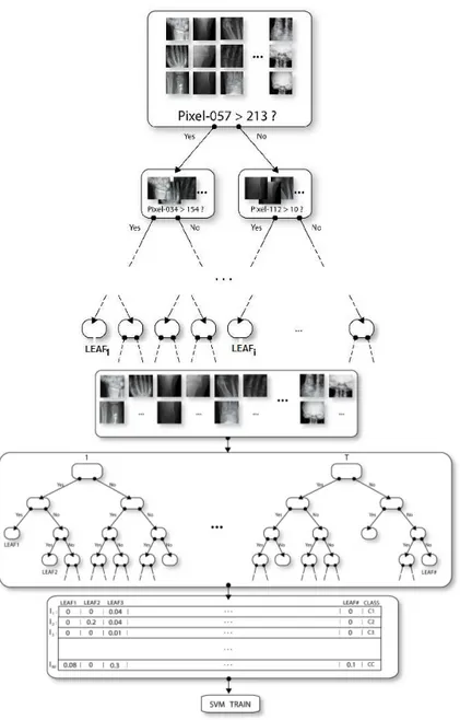
For instance, a test image that has been classified by the extra-trees with a probability of 0.9 means that a great number of subwindows have been assigned a high probability of

Use the Tfid- fVectorizer tool provided by scikit-learn to convert the text data into TF-IDF feature vector, using the logistic regression, support vector machine, naive

Figure 2 shows the performance on a random validation dataset (20 percent of training data) using ensemble of models trained with over-sampling, threshold moving and error

1) Taking into account the relationship between HSI channels by calculating the correlation, constructing a linear predictor of the next channel value from the

As vast research in sensors to detect physiological changes relation to emotion has been conducted in the field of autonomic response and the emotional state in a learning context

References

Ciresan, D.C., Meier, U., Schmidhuber, J., 2012. Multi-column deep neural networks for image classification, in: Computer Vision and Pattern Recognition, pp. 3642–3649.
Criminisi, A., Shotton, J. (Eds.), 2013. Decision Forests for Computer Vision and Medical Image Analysis. Ad-vances in Computer Vision and Pattern Recognition, Springer.
Delga, A., Goffin, F., Marée, R., Lambert, C., Delvenne, P., 2014. Evaluation of cellsolutions bestprep(r) au-tomated thin-layer liquid-based cytology papanicolaou slide preparation and bestcyte(r) cell sorter imaging system. Acta Cytologica 58, 469–77.
Dumont, M., Marée, R., Wehenkel, L., Geurts, P., 2009. Fast multi-class image annotation with random subwin-dows and multiple output randomized trees, in: Proc. VISAPP, pp. 196–203.
Everingham, M., Van Gool, L., Williams, C.K.I., Winn, J., Zisserman, A., 2010. The PASCAL Visual Ob-ject Classes (VOC) challenge. International Journal of Computer Vision 88, 303–338.
Gehler, P.V., Nowozin, S., 2009. On feature combina-tion for multiclass object classificacombina-tion, in: Proc. IEEE International Conference on Computer Vision (ICCV), pp. 221–228.
Geurts, P., Ernst, D., Wehenkel, L., 2006. Extremely ran-domized trees. Machine Learning 36, 3–42.
Huang, G.B., Ramesh, M., Berg, T., Learned-Miller, E., 2007. Labeled Faces in the Wild: A Database for Studying Face Recognition in Unconstrained Environ-ments. Technical Report 07-49. University of Mas-sachusetts, Amherst.
Jeanray, N., Marée, R., Pruvot, B., Stern, O., Geurts, P., Wehenkel, L., Muller, M., 2015. Phenotype classifica-tion of zebrafish embryos by supervised learning. PLos ONE 10, e0116989.
Kotseruba, T., Cumbaa, C., Jurisica, I., 2012. High-throughput protein crystallization on the world commu-nity grid and the gpu. Journal of Physics: Conference Series 341.
Le, Q.V., Ngiam, J., Chen, Z., Chia, D., Koh, P.W., Ng, A.Y., 2010. Tiled convolutional neural networks, in: Lafferty, J., Williams, C., Shawe-Taylor, J., Zemel, R., Culotta, A. (Eds.), Advances in Neural Information Processing Systems 23, pp. 1279–1287.
LeCun, Y., Bengio, Y., Hinton, G., 2015. Deep learning. Nature 521, 436–444.
Lintott, C.J., Schawinski, K., Slosar, A., Land, K., Bam-ford, S., Thomas, D., Raddick, M.J., Nichol, R.C., Sza-lay, A., Andreescu, D., Murray, P., Vandenberg, J., 2008. Galaxy Zoo: morphologies derived from visual inspection of galaxies from the Sloan Digital Sky Sur-vey. Monthly Notices of the Royal Astronomical Soci-ety 389, 1179–1189.
Marée, R., Geurts, P., Piater, J., Wehenkel, L., 2004. A generic approach for image classification based on decision tree ensembles and local sub-windows, in: Hong, K.S., Zhang, Z. (Eds.), Proceedings of the 6th Asian Conference on Computer Vision, pp. 860–865. Marée, R., Geurts, P., Piater, J., Wehenkel, L., 2005.
Ran-dom subwindows for robust image classification, in: Proc. IEEE CVPR, IEEE. pp. 34–40.
Marée, R., Geurts, P., Visimberga, G., Piater, J., We-henkel, L., 2003. An empirical comparison of ma-chine learning algorithms for generic image classifica-tion, in: Coenen, F., Preece, A., Macintosh, A. (Eds.), Proc. 23rd SGAI AI„ Springer. pp. 169–182.
Marée, R., Geurts, P., Wehenkel, L., 2007. Random sub-windows and extremely randomized trees for image classification in cell biology. BMC Cell Biology sup-plement on Workshop of Multiscale Biological Imag-ing, Data Mining and Informatics 8.
Marée, R., Geurts, P., Wehenkel, L., 2009. Content-based image retrieval by indexing random subwindows with randomized trees. IPSJ Transactions on Computer Vi-sion and Applications 1, 46–57.
(13)
Marée, R., Rollus, L., Stévens, B., Hoyoux, R., Louppe, G., Vandaele, R., Begon, J.M., Kainz, P., Geurts, P., Wehenkel, L., 2015. Collaborative analysis of multi-gigapixel imaging data using cytomine. Under revision
URL:http://www.cytomine.be/.
Moosmann, F., Nowak, E., Jurie, F., 2008. Randomized clustering forests for image classification. IEEE Trans-actions on PAMI 30, 1632–1646.
Oliva, A., Torralba, A., 2001. Modeling the shape of the scene: a holistic representation of the spatial envelope. International Journal of Computer Vision 42, 145–175. Orlov, N., Shamir, L., Macura, T., Johnston, J., Eckley, D.M., Goldberg, I., 2008. Wnd-charm: Multi-purpose image classification using compound transforms. Pat-tern Recognition Letters 29, 1684–1693.
Pinto, N., Dicarlo, J., Cox, D., 2008. Establishing good benchmarks and baselines for face recognition, in: ECCV 2008 Faces in ’Real-Life’ Images Workshop. Pinto, N., Doukhan, D., DiCarlo, J., Cox, D., 2009. A high-throughput screening approach to discovering good forms of biologically-inspired visual representa-tion. PLoS Computational Biology 5.
Quattoni, A., A.Torralba, 2009. Recognizing indoor scenes, in: IEEE Conference on Computer Vision and Pattern Recognition (CVPR), pp. 413–420.
Ranzato, M., Krizhevsky, A., Hinton, G.E., 2010. Fac-tored 3-way restricted boltzmann machines for model-ing natural images. Journal of Machine Learnmodel-ing Re-search - Proceedings Track 9, 621–628.
Shamir, L., 2008. Evaluation of face datasets as tools for assessing the performance of face recognition method. International Journal of Computer Vision 79, 225–230. Stern, O., Marée, R., Aceto, J., Jeanray, N., Muller, M., Wehenkel, L., Geurts, P., 2011. Automatic localization of interest points in zebrafish images with tree-based methods, in: Proc. 6th IAPR International Conference on Pattern Recognition in Bioinformatics, Springer-Verlag. pp. 179–190.
Xiao, J., Hays, J., Ehinger, K., Oliva, A., Torralba, A., 2010. Sun database: Large-scale scene recognition from abbey to zoo, in: Proc. IEEE Conference on Com-puter Vision and Pattern Recognition (CVPR2010), pp. 3485–3492.
Supplementary Material
Figure
Figure 1: Left: A single tree induced from a training set of random subwindows, using node tests with single pixel thresholding, for the ET-FL scheme
Figure 3: Results averaged over all 80 datasets for ET-FL variant: First column: Average of error rates for all datasets with subwindow size intervals (1st row), image representation (2nd), number of random tests (3rd), number of trees (4th), minimum node
Figure 2: Summary of the best error rate obtained for each dataset without optimizations, gathered from Supplementary Tables II to XII
Figure 5: Several datasets for which larger subwindow sizes yield lowest error rates.
Références
Documents relatifs