On the relation between the maximum entropy Principle and the principle of Least effort : The continuous case

HAL Id: hal-00606900

https://hal.archives-ouvertes.fr/hal-00606900

Submitted on 7 Jul 2011

HAL is a multi-disciplinary open access

archive for the deposit and dissemination of sci-entific research documents, whether they are pub-lished or not. The documents may come from teaching and research institutions in France or

L’archive ouverte pluridisciplinaire HAL, est destinée au dépôt et à la diffusion de documents scientifiques de niveau recherche, publiés ou non, émanant des établissements d’enseignement et de recherche français ou étrangers, des laboratoires

On the relation between the maximum entropy Principle

and the principle of Least effort : The continuous case

Abdelatif Agouzal, Thierry Lafouge

To cite this version:

Abdelatif Agouzal, Thierry Lafouge. On the relation between the maximum entropy Principle and the principle of Least effort : The continuous case. Journal of Informetrics, Elsevier, 2008, 2 (1), pp.75-88. �hal-00606900�

On the relation between the Maximum Entropy Principle and the Principle

of Least Effort: the continuous case

Abdelatif, AGOUZAL1; Thierry LAFOUGE2

1_{Université de Lyon, France; Université Lyon 1, Institut Camille Jordan, CNRS U.M.R. 5208,}

Villeurbanne, F-69622, France

2_{Université de Lyon, France; Université Lyon 1, ELICO, Villeurbanne, F-69622, France}

Abstract

The Maximum Entropy Principle (MEP) maximises the entropy provided that the effort remains constant. The Principle of Least Effort (PLE) minimises the effort provided that the entropy remains constant. The paper investigates the relation between these two principles. In some kinds of effort functions, called admissible, it is shown that these two principles are equivalent. The results are illustrated by the size-frequency statistical distribution met in infometry in Information Production Processes.

Keywords: Maximum Entropy Principle; Principle of Least Effort; Effort function; Inverse power function

Introduction

The article is divided into two parts. In the first, through the signal theory, we mathematically formulate the equivalence of the two principles, Maximum Entropy Principle with constant effort, and the Principle of Least Effort with constant entropy. Then we situate these problems within the processes of producing and using information in infometry. In the second part, we mathematically demonstrate equivalence by introducing the concept of admissible effort function. To conclude, we return to the information production processes to clarify the properties of the usual functions that model the information production processes.

1

Definitions and context

1.1 Information theory

In 1948 Shannon (Shanon, 1993) worked out a statistical theory on the transmission of electrical signals. This statistical theory of information stipulates that the more the states of a system are equiprobable, the more the process produces information. The theoretical bases used in this article come from this theory. Here, we uniquely consider density functions of probability

µ

defined from

[

1

,..

∞

[

with real positive values and verifying:

∫

∞

=

1

1

)

( dx

x

µ

We call effort function any continuous

f

function defined from

[

1

,..

∞

[

with real positive values. For each couple

(

µ

,

f

)

, we define two quantities,

H

1 average information content, called entropy and

F

average effort:

∫

∞

=

∫

∞

−

=

1 1

,

)

(

)

(

,

))

(

(

)

(

x

Ln

x

dx

F

f

x

x

dx

f

H

µ

µ

F

is necessarily positive. Let us now define two important optimization principles: Maximum Entropy Principle (MEP) and Principle of Least Effort (PLE).

Maximum Entropy Principle (MEP)

The MEP maximises the entropy provided that the effort remains constant. Principle of Least Effort (PLE)

The PLE minimises the effort provided that the entropy remains constant. Mathematical formulation of the two principles

With

H

,

F

positive, two real numbers, and

f

an effort function, we define the sets of functions:

∫

∞

=

=

−

∫

∞

≥

=

Α

1 1

)

(

(

)

(

,

1

)

(

,

0

)

(

H

µ

µ

x

dx

H

µ

x

Ln

µ

x

dx

∫

∞

=

=

∫

∞

≥

=

1 1

)

(

)

(

,

1

)

(

,

0

)

(

F

x

dx

F

x

f

x

dx

C

µ

µ

µ

With these notations, MEP and PLE are written:

∫

∞ ∈

−

⇔

1 ) (

(

(

x

)

Ln

(

(

x

))

dx

)

Max

MEP

F C

µ

µ

µ

∫

∞ ∈

⇔

1 ) (

(

(

x

)

f

(

x

)

dx

)

Min

LEP

_{µ A H}

µ

Our aim is to show, under certain conditions, that these two principles are equivalent. We will situate the problem within the sphere of infometry and recall results obtained in earlier work.

1.2 Informetrics and entropy aspects

1.2.1 Information Production Process and Inverse power law

Statistical regularities observed in producing or using information have been studied for a long time. In practice, the production function has similar characteristics in very diverse situations of production or use of information.

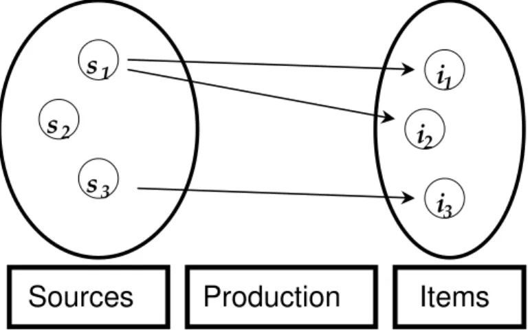
These models can be represented by the diagram of Fig.1, introduced into informetric systems by Leo Egghe (Egghe, 1990) and called “Information Production Process” (IPP). An

IPP is a triplet made up of a bibliographical source, a production function, and all the

elements (items) produced.

Figure 1: Schematic representation of an Information Production Process

- Authors (sources) write articles (items)

- Words in a text (sources) produce occurrences of words in the text (items) - Web pages (sources) contain links (items)

- Web sites (sources) are visited (items)

- Requests (sources) through a search engine are sent by users (items).

In all quoted examples, if we quantify the production of the items by the sources with a size frequency function, this one is decreasing with a long tail and a gap between a high number of sources producing few items and a small number of sources producing a lot. Their most current mathematical formulation is that of an inverse power function, usually called a lotkaian informetric distribution (Egghe, 2005), the corresponding density probability

ν

_λ is:

[

∞

[

∈

1

,..

x

,

ν

_λ

(

)

=

λ

−

_λ

1

,

λ

>

1

x

x

The calculation of the entropy (Yablonsky , 1981)

H

(

λ

)

according to

λ

gives:

1

,

1

)

1

1

(

)

(

>

−

+

−

=

λ

λ

λ

λ

λ

Ln

H

It is easy to show that the entropy is a decreasing function of

λ

. The classical interpretation of Lotka’s law (Lotka, 1926) is found, e.g. the higher

λ

is, the bigger is the gap between the number of scientists who produce a lot compared to the number of scientists who produce a little, knowing that there are few scientists who produce a lot compared to the number of scientists who produce a little.

Thus, the two following questions arise:

s

₁

s

₂

s

₃

i

₁

i

2

i

₃

1) For a given quantity of effort, what is the connection between the random distribution of the sources and the effort function when the quantity of information produced by the sources is maximized?

2) For a given quantity of information, what is the connection between the random distribution of the sources and the effort function when the quantity of effort produced by the source is maximized?

1.2.2 Previous results

1.2.2.1 Finite discrete case

Suppose

µ

is a finite discrete distribution, so we have

m

∈

N

probabilities

p

₁

,

p

₂

,..,

p

_m so that

∑

=

=

m r r

p

1

1

, the entropy of such a system is defined as

∑

=

−

=

m r r r

Ln

p

p

H

1

)

(

. Let

0

>

r

F

denote the effort function (

r

=

1

,..,

m

) the quantity of effort is defined

as

(

)

1 .

∑

=

=

m r r r r

p

Ln

p

E

F

. In () we prove the following result, if we suppose

p

₁

,

p

₂

,..,

p

_mis a decreasing sequence MEP and PLE are equivalent. In the conclusion to this article we provided a complete explanation of Zip's law (Egghe and Lafouge, 2006) or Lotka's law as a decreasing function.

An incomplete demonstration of the result of equivalence in the continuous case was subsequently proposed (see paragraph 1.2.2.2). The aim of this article is to generalize this result.

1.2.2.2 Exponential Informetric Process

In Lafouge and Prime Claverie (Lafouge and Prime Claverie, 2005) we assume that an item produced requires a certain amount of effort and therefore we define the exponential informetric process by introducing the effort function (see Fig. 2). The effort function denotes the amount of effort from a source to produce items.

s

₁

s

2

s

₃

i

1

i

₂

i

₃

Figure 2: Schematic representation of an informetric process using the effort function

With

f

a strictly increasing unbounded effort function,

λ

a positive number where we have the condition:

∞

<

−

∫

∞ 1

))

(

exp(

)

(

x

f

x

dx

f

λ

[1]

Since

f

is strictly increasing, unbounded, we can easily show the condition:

∫

∞

∞

<

−

1

))

(

exp(

λ

f

x

dx

Therefore, we call the following density function Exponential Informetric Process:

∫

∞

−

−

=

1

))

(

exp(

))

(

exp(

)

(

dx

x

f

x

f

x

λ

λ

ν

_λ

∫

∞ 1

)

(

)

(

x

x

dx

f

ν

_λ corresponds to the average

F

of effort produced by the Exponential

Informetric Process. The following results explain the relationship between average amount of effort and entropy.

We have shown (Lafouge and Prime Claverie, 2005) the following results: (i)

ν

_λis decreasing,

(ii) The two principles maximum MEP and PLE are verified simultaneously, (iii)

H

=

Ln

(

k

)

+

λ

F

where

∫

∞

−

=

1

))

(

exp(

f

x

dx

k

λ

and

H

corresponds to the entropy.

This result partly resolves the problem of the equivalence of the two principles given in paragraph 1.1. In fact, the condition is sufficient for these two principles to be equivalent. In the two preceding demonstrations, finite and discrete cases (equivalence) and in the continuous case (sufficient condition), we calculate a solution for the MEP that plays a central role in mechanical statistic,

))

(

exp(

)

(

x

C

λ

f

x

ν

=

−

where C is a constant,

λ

a positive number and

f

an effort function. This distribution, constructed with the MEP, is known under the name of Bolzmann distribution. To our knowledge, there is no mathematical demonstration of the equivalence of these two principles (MEP and PLE) in the continuous case.

Note

Demonstration (ii) of the preceding result supposes, when we write the

equality

∫

∞

−

=

1

))

(

exp(

)

(

x

f

x

dx

f

F

λ

, the existence of a unique

λ

verifying this

inequality. The demonstration given in paragraph 2 will clarify this point.

1.2.2.3 Effort function and inverse power law

With the preceding formalism, the density function corresponding to an inverse power is written:

x

∈ ,..

[

1

∞

[

,

ν

_λ

(

x

)

=

(

λ

−

1

)

exp(

−

(

λ

−

1

)

Ln

(

x

))

,

λ

>

1

The calculation of the amount of effort according to

λ

gives:

1

,

1

1

)

(

>

−

=

λ

λ

λ

F

The logarithmic function is the effort function corresponding to the Lotka distributions. When we are interested for example in the production of words in a text and when we express this regularity using the formalism of Zipf’s law (see Conclusion). In (Egghe and Lafouge, 2006, p 8), this hypothesis is formulated thus: the cost (effort) of using a word with

i

,

(

i

=

1

,

2

,

3

,....)

letters is proportional to

i

hence to

Log

_N

(r

)

where

N

is the number of different letters and

r

is the rank of a word with

i

letters.

Moreover the results presented in (Lafouge and Smolczeswska, 2006) show that if an effort function

f

verifies the condition,

1

,

)

(

)

(

>

=

∞ →

λ

λ

x

Ln

x

f

Limit

_x

we have an Exponential Informetric Process.

We will now directly demonstrate the equivalence of the two principles using the continuous case with effort functions, strictly increasing, unbounded and verifying the condition [1].

2.

Characterising the Maximum Entropy Principle in terms of

the Principle of Least Effort

2.1 Main results

2.1.1 Preliminary and notation

In all that follows

f

denotes a strictly increasing unbounded, effort function .

f

will be called admissible if there is also a real number

λ

₀ verifying the condition

∫

∞

∞

<

−

1 0

(

))

exp(

)

(

x

f

x

dx

f

λ

Lemma 2.0

With

f

an admissible effort function, there exists a reality

σ

(

f

)

≥

0

so that

∫

∞

∞

<

−

≤

>

∀

1

))

(

exp(

)

(

0

),

(

f

f

x

λ

f

x

dx

σ

λ

Proof

f

being admissible,

there exists

λ

₀

∈

ℜ

so that

∫

∞

∞

<

−

≤

1 0

(

))

exp(

)

(

0

f

x

λ

f

x

dx

f

being increasing

∀

λ

>

λ

₀ we have,

∫

∫

∞ ∞

∞

<

−

<

−

≤

1 1 0

(

))

exp(

)

(

))

(

exp(

)

(

0

f

x

λ

f

x

dx

f

x

λ

f

x

dx

Moreover, it is clear that

∫

∞

∞

+

=

1

)

(

x

dx

f

, consequently

λ

₀ is strictly positive. We can then

define the following real number:

∫

∞

∞

<

−

<

>

=

1

))

(

exp(

)

(

0

,

0

inf

)

(

f

λ

f

x

λ

f

x

dx

σ

We will now define two functions

H

and

F

quantifying the entropy and effort of a density function

µ

,

∫

∞

=

1

1

)

( dx

x

ν

We define the entropy of

µ

,

∫

∞

−

=

1

))

(

(

)

(

)

(

x

Ln

x

dx

H

µ

µ

µ

which can be infinite and the quantity of effort of

µ

,

∫

∞

=

1

)

(

)

(

)

(

x

f

x

dx

F

µ

µ

Let

H

and

F

two constants,

A

(H

)

and

C

(F

)

the set of functions defined in the introduction,

∀

λ

>

σ

( f

)

we put:

∫

∞

−

=

1

))

(

exp(

f

x

dx

k

λ

k

x

f

x

)

exp(

(

))

(

λ

ν

_λ

=

−

∫

∞

−

=

1

))

(

(

)

(

)

(

x

Ln

x

dx

H

λ

ν

_λ

ν

_λ

∫

∞

=

1

)

(

)

(

)

(

f

x

x

dx

F

λ

ν

_λ

The following results are simple consequences of the preceding definitions.

Lemma 2.1

),

( f

σ

λ

>

∀

the entropy

H

(

λ

)

of

ν

_λ is finite. Proof

∞ ∞

)

(k

Ln

F

+

=

λ

Also, the two functions are defined:

∫

∞

−

−

−

=

1

))

)

(

(

exp(

(

)

(

Ln

f

x

F

dx

Z

λ

λ

∫

∞

−

−

−

=

1

)

)

)

(

exp(

(

1

)

(

Ln

f

x

H

dx

R

λ

λ

λ

Lemma 2.2

With

µ

∈

C

(F

)

,

λ

>

σ

( f

)

, we have:

∫

∞

=

1

)

(

))

(

(

)

(

ν

λ

µ

x

Ln

_λ

x

dx

Z

Proof

∫

∫

∫

∞ ∞ ∞

−

−

−

=

1 1 1

)

))

(

exp(

(

)

(

)(

(

))

(

(

)

(

x

Ln

ν

x

dx

µ

x

λ

f

x

Ln

λ

f

x

dx

dx

µ

_λ

)

)

(

exp(

)

(exp(

)

))

(

exp(

(

.

1 1

∫

∫

∞

−

=

−

∞

−

−

−

=

λ

F

Ln

λ

f

x

dx

Ln

λ

F

λ

f

x

dx

dx

F

x

f

Ln

(

exp(

(

(

)

))

1

∫

∞

−

−

−

=

λ

Lemma 2.3

Let

ν

_λ

∈

C

(F

)

, we have

(

(

)

)

exp(

(

))

0

1

=

−

−

∫

∞

dx

x

f

F

x

f

λ

Proof

)

(F

C

∈

λ

ν

, hence

F

k

dx

x

f

x

f

−

=

∫

∞ 1

))

(

exp(

)

(

λ

∫

∫

∞ ∞

−

−

=

−

−

1 1

))

(

exp(

)

(

))

(

exp(

)

)

(

(

f

x

F

λ

f

x

dx

f

x

λ

f

x

dx

k

F

0

=

−

=

k

F

k

F

2.1.1 Equivalence theorem

We can now state the equivalence theorem of the two principles by characterizing the solutions of the MEP and the PLE using the functions

Z

(

λ

)

and

R

(

λ

)

.

Theorem

With

f

an admissible effort function, we have the following results:

(i) _{( )} ) (

(

(

))

)

(

0

Max

H

_{C F}

Sup

Z

_{λ σ f} µ

λ

µ

_∈

≥

_>

≥

Also, if there is a a real number

λ

₀ so that

(

)

0

∈

C

F

λ

ν

then this real number is unique and we have:

)

(

))

(

(

)

(

)

(

λ

₀

Max

H

µ

_{µ ( )}

Sup

Z

λ

_{λ σ( )}

Z

λ

₀

H

=

_{∈C F}

=

_{> f}

=

(ii) _{( )} ) (

(

(

))

)

(

0

Min

F

_{A H}

Sup

R

_{λ σ f} µ

λ

µ

_∈

≥

_>

≥

Also, if there is a a real number

λ

₁ so that

(

)

1

∈

A

H

λ

ν

then this real number is unique and we have:

)

(

))

(

(

)

(

)

(

λ

₁

MinF

µ

_{µ ( )}

Sup

R

λ

_{λ σ( )}

R

λ

₁

F

=

_{∈A H}

=

> _f

=

(iii) If

H

=

−

Z

(

λ

₁

)

or

F

=

R

(

λ

₀

)

then 1 0 λ λ

ν

ν

=

(i) characterizes the solution of the MEP, in other words maximizing the entropy subject to a constant effort, (ii) characterizes the solution of the PLE, in other words minimizing the effort subject to constant entropy. Finally, if the information content

H

and quantity of effort

F

are linked, in other words if

H

=

−

Z

(

λ

₁

)

or if

F

=

R

(

λ

₀

)

, the two principles are equivalent. We note that in this case we find the result (iii) of paragraph 1.2.2.2,

H

=

λ

1

F

+

Ln

(

k

)

or

)

(

0

F

Ln

k

H

=

λ

+

.

Before solving this problem, we will give arguments by a formal result to demonstrate (i) as follows. We have,

∫

∫

∞ ∞

−

−

−

−

−

=

1

))

)

(

(

exp(

))

)

(

(

exp(

)

(

dx

F

x

f

dx

F

x

f

F

f

d

dZ

λ

λ

λ

λ

d

dZ

(

λ

₀

)

=

0

, which means that

Z

(

λ

₀

)

is an extremum of function

Z

.

2.2 Demonstration of the equivalence theorem

Preliminary

For this problem to be of mathematical interest, we need to show that

A

(H

)

and

C

(F

)

are not empty and to suppose additional hypotheses regarding the effort function

f

so that the maximum entropy is finite. Readers should refer to points 1,2 and 3 in the appendix for these demonstrations.

We will solve this problem uniquely through the use of elementary analytical arguments.

Lemma 2.4

Let two real numbers

y

≥

0

and

z

>

0

, we have:

(i)

yLn

(

y

)

≥

y

−

z

+

yLn

(

z

)

, and strict inequality if, and only if,

y

≠

z

(ii)

yLn

(

y

)

−

zLn

(

z

)

≥

(

1

+

Ln

(

z

))(

y

−

z

)

Proof

(ii) is immediately deduced from (I).

For

y

=

0

and

y

=

z

, the result is trivial. With

y

>

0

,

z

>

0

,

y

≠

z

, we put

y

z

t

=

, we have

1

)

(

,

1

,

0

≠

<

−

>

∀

t

t

Ln

t

t

, hence

y

y

z

y

Ln

z

Ln

(

)

−

(

)

<

−

.

Proposition 2.1

For any admissible function, we have:

) ( ) (

(

)

)

(

0

≥

Max

H

µ

_{µ∈C F}

≥

Sup

Z

λ

_{λ>σ f} Proof

With

µ

∈

C

(

F

)

,

λ

>

σ

(

f

)

using the result (i) of lemma 2.4 with

y

=

µ

and

z

=

ν

_λ, and by integrating the functions, we have:

∫

∫

∞

≥

∫

∞

−

+

∞ 1 1 1

))

(

(

)

(

))

(

)

(

(

))

(

(

)

(

x

Ln

µ

x

dx

µ

x

v

_λ

x

dx

µ

x

Ln

ν

_λ

x

dx

µ

we know,

0

1

1

))

(

)

(

(

1

=

−

=

−

∫

∞

µ

x

v

_λ

x

dx

,

consequently

dx

x

Ln

x

H

∫

∞

≥

−

1

))

(

(

)

(

)

(

µ

µ

ν

_λ

thus according to lemma 2.2

)

(

)

(

µ

Z

λ

H

≥

−

hence

)

(

)

(

),

(

),

(

λ

σ

µ

λ

µ

∈

C

F

∀

>

f

−

H

≥

Z

∀

Also, according to point 2 in the appendix, there is a function

µ

_z

∈

C

(F

)

verifying

µ

_z

≤

1

, consequently

µ

_z

Ln

(

µ

_z

)

≤

0

and thus,

) ( ) (

(

)

)

(

0

≥

Max

H

µ

_{µ∈C F}

≥

Sup

Z

λ

_{λ>σ f}

Proposition 2.2

With

f

an admissible effort function, for any density function

µ

we have

µ

ν

σ

λ

>

_λ

≠

∀

(

f

),

, the following inequality:

dx

x

f

x

x

dx

x

Ln

x

dx

x

Ln

x

)

(

(

))

(

)

(

(

))

(

(

)

(

))

(

)

(

1 1 1

∫

∫

∞

µ

µ

−

∫

∞

ν

_λ

ν

_λ

>

λ

∞

ν

_λ

−

µ

Proof

With

λ

>

σ

( f

)

so that

ν

_λ

≠

µ

,

using lemma 2.4 (ii) with

y

=

µ

and

z

=

ν

_λ, we have the inequality:

))

(

(

1

))(

(

)

(

(

))

(

(

)

(

))

(

(

)

(

x

Ln

µ

x

ν

_λ

x

Ln

ν

_λ

x

µ

x

ν

_λ

x

Ln

ν

_λ

x

µ

−

≥

−

+

By integrating the right member, we obtain:

∫

∫

∞

−

+

∞

−

1 1

))

(

(

))

(

)

(

(

))

(

)

(

(

µ

x

ν

_λ

x

dx

µ

x

ν

_λ

x

Ln

ν

_λ

x

dx

However

0

1

1

))

(

)

(

(

1

=

−

=

−

∫

∞

µ

x

ν

_λ

x

dx

Consequently,

dx

k

Ln

x

f

x

x

dx

x

Ln

x

x

)

(

))

(

(

))

(

(

)

(

))

(

(

)

(

))

(

(

1 1

−

−

−

=

−

∫

∫

∞

µ

ν

_λ

ν

_λ ∞

µ

ν

_λ

λ

Hence

dx

x

f

x

x

)

(

))

(

(

))

(

(

1

λ

ν

µ

−

_λ

−

=

∫

∞

Lemma 2.5

For any couple of real numbers

z

₁

,

z

₂

,

we have the following inequality:

)

exp(

)

(

)

exp(

)

exp(

−

z

₂

−

−

z

₁

≥

z

₁

−

z

₂

−

z

₁ Proof

We have the strict inequality if

z

₁

≠

z

₂. Let us suppose

z

₁

<

z

₂, according to the mean theorem, there is

z

,

z

₁

<

z

<

z

₂, verifying the equality:

)

exp(

)

(

)

exp(

)

exp(

z

₂

−

z

₁

=

−

z

₂

−

z

₁

−

z

The inequality is then written:

)

exp(

)

(

)

exp(

)

(

z

₁

−

z

₂

−

z

≥

z

₁

−

z

₂

−

z

₁ with

)

exp(

)

exp(

−

z

≤

−

z

₁ We do the same if

z

₂

<

z

₁

We will show the most important intermediate result, namely the sets

C

(

F

)

are sets of uniqueness for the functions

0

λ

ν

. More precisely, we demonstrate the result below.

Proposition 2.3

With

f

an admissible function, there exists at most a function

0

λ

ν

belonging to

C

(

F

)

verifying the inequality:

Sup

Z

(

λ

)

_λ>σ(f)

=

Z

(

λ

₀

)

Proof

1) Uniqueness

Let us suppose

λ

₁

≠

λ

₂ so that

,

(

)

2

1 λ

∈

C

F

λ

ν

ν

, according to lemma 2.1 we know that the entropy of

ν

_λ is finite, by applying proposition 2.2 twice, we obtain

0

)

(

))

(

)

(

(

))

(

(

)

(

))

(

(

)

(

1 1 1 1 2 1 1 1 2 2

−

>

∫

−

=

∫

∞

ν

_λ

x

Ln

ν

_λ

x

dx

∫

∞

ν

_λ

x

Ln

ν

_λ

x

dx

λ

∞

ν

_λ

x

ν

_λ

x

f

x

dx

And in the same way

0

)

(

))

(

)

(

(

))

(

(

)

(

))

(

(

)

(

1 2 1 1 1 2 2 2 1 1

−

>

∫

−

=

∫

∞

ν

_λ

x

Ln

ν

_λ

x

dx

∫

∞

ν

_λ

x

Ln

ν

_λ

x

dx

λ

∞

ν

_λ

x

ν

_λ

x

f

x

dx

which is contradictory and consequently there is at most one item belonging to

C

(

F

)

. 2) Existence

Let a function

(

)

0

∈

C

F

λ

ν

, according to lemma 2.5, we can write

y

z

y

z

₂

=

λ

,

₁

=

λ

₀ ,

exp(

−

λ

y

)

≥

exp(

−

λ

₀

y

)

−

y

(

λ

−

λ

₀

)

exp(

−

λ

₀

y

)

By putting

y

=

f

(

x

)

−

F

and integrating,

dx F x f F x f dx F x f dx F x f( ) )) exp( ( ( ) )) ( ) ( ( ) )exp( ( ( ) )) ( exp( 0 1 1 1 0 0 − − − − − − − ≥ − −

∫

∞ λ

∫

∞ λ λ λ

∫

∞ λ

)

(

0

C

F

v

_λ

∈

we know according to lemma 2.3,

0

))

)

(

(

exp(

)

)

(

(

1 0

−

=

−

−

∫

∞

f

x

F

λ

f

x

F

dx

consequently,

∫

∞

−

−

≥

∫

∞

−

−

1 1 0

(

(

)

))

exp(

))

)

(

(

exp(

λ

f

x

F

dx

λ

f

x

F

dx

hence

)

(

)

(

λ

Z

λ

₀

Z

≤

and thus

)

(

)

(

λ

_{λ σ( )}

Z

λ

₀

Z

Sup

_{> f}

≤

Theorem 2.1

We suppose that there is a real number

λ

₀

>

σ

(

f

)

so that

(

)

0

∈

C

F

λ

ν

, then this real number is unique and moreover:

∫

∞ ∈ >

=

=

=

−

1 ) ( 0 ) (

(

)

(

)

(

)

(

(

))

)

(

(

0 0

x

Ln

x

dx

MaxH

Z

Z

Sup

λ

_{λ σ f}

λ

µ

_{µ C F}

ν

_λ

ν

_λ Proof

Uniqueness and characterization by the function

Z

are consequences of proposition 2.3. With

0

),

(

µ

ν

_λ

µ

∈

C

F

≠

using the inequality of proposition 2.2,

dx

x

f

x

x

dx

x

Ln

x

dx

x

Ln

x

)

(

(

))

(

)

(

(

))

(

(

)

(

))

(

)

(

1 1 1 0 0

∫

∫

∞

µ

µ

−

∫

∞

ν

_λ

ν

_λ

>

λ

∞

ν

_λ

−

µ

However

0

)

(

))

(

)

(

(

1 0

−

=

−

=

∫

∞

ν

_λ

x

µ

x

f

x

dx

F

F

Thus

∫

∞

<

−

∫

∞

−

1 1

))

(

(

)

(

))

(

(

)

(

0 0

x

Ln

x

dx

dx

x

Ln

x

µ

ν

_λ

ν

_λ

µ

Note

It is essential to suppose that the function

0

λ

ν

is well defined because the whole definition of the function

Z

is greater than

]

σ

(

f

),..

∞

[

, as the following example shows. With the effort function

f

(

x

)

=

Ln

(

x

+

1

)

+

Ln

(

Ln

2

(

x

+

1

)),

we show

∫

∞

∞

<

−

1

)

(

exp(

f

x

dx

, therefore

)

1

(

Z

is well defined whereas

∫

−

=

∞

∞

dx

x

f

x

f

(

)

exp(

(

))

1 .

In the same way, with

H

a real number we consider the function

R

(

λ

)

, we demonstrate proposition 2.4 using the same techniques as previously.

Proposition 2.4

With

f

an admissible function, there is at most a function

1

λ

ν

belonging to

A

(

H

)

verifying the inequality:

Sup

R

(

λ

)

_λ>σ(f)

=

R

(

λ

₁

)

We can now demonstrate the result (ii) of the equivalence theorem.

Theorem 2.2

We suppose that there is a reality

λ

₁

>

σ

(

f

)

so that

(

)

1

∈

A

H

λ

ν

, then this reality is unique and also:

∫

∞ ∈ >

=

=

=

1 ) ( 1 ) (

(

)

(

)

(

)

(

)

))

(

(

1

x

f

x

dx

F

Min

R

Z

Sup

H A f µ λ σ λ

λ

µ

ν

λ

Proof

Uniqueness and characterization by the function

R

are consequences of proposition 2.3. With

µ

∈

A

(

H

)

, using the inequality of proposition 2.2 we obtain,

dx

x

f

x

x

dx

x

Ln

x

dx

x

Ln

x

)

(

(

))

(

)

(

(

))

(

(

)

(

))

(

)

(

1 1 1 1 1 1

∫

∫

∞

µ

µ

−

∫

∞

ν

_λ

ν

_λ

>

λ

∞

ν

_λ

−

µ

dx

x

f

x

x

H

H

(

(

)

(

))

(

)

0

1 1

∫

∞

−

>

−

=

λ

ν

_λ

µ

consequently, since

λ

>

0

,

∫

∞

<

∫

∞ 1 1

)

(

)

(

)

(

)

(

1

x

dx

f

x

x

dx

x

f

ν

_λ

µ

using theorems 2.1 and 2.2, we obtain the equivalence theorem.

Theorem 2.3

Let a positive, unbounded, strictly increasing, continuous function, we suppose that there exists

λ

₀

∈

ℜ

so that:

∞

<

−

1. There is a real number

σ

(

f

)

so that:

),

(

f

σ

λ

>

∀

≤

∫

−

<

∞

∞ 1

))

(

exp(

)

(

0

f

x

λ

f

x

dx

2. We have ) ( ) (

(

)

)

(

0

Max

H

_{C F}

Sup

Z

_{λ σ f} µ

λ

µ

_∈

≥

_>

≥

Also, if there is a real number

λ

₀ so that

(

)

0

∈

C

F

λ

ν

then this real number is unique and we have:

)

(

)

(

)

(

)

(

λ

₀

Max

H

µ

_{µ ( )}

Sup

Z

λ

_{λ σ( )}

Z

λ

₀

H

_f F C

=

=

=

_{∈ >} where

∫

∞

−

−

−

=

1

))

)

(

(

exp(

(

)

(

Ln

f

x

F

dx

Z

λ

λ

3. We have ) ( ) (

(

)

)

(

0

Min

F

_{A H}

Sup

R

_{λ σ f} µ

λ

µ

_∈

≥

_>

≥

Also, if there is a reality

λ

₁ so that

(

)

1

∈

A

H

λ

ν

then this real number is unique and we have:

)

(

)

(

)

(

)

(

λ

₁

MinF

µ

_{µ ( )}

Sup

R

λ

_{λ σ( )}

R

λ

₁

F

_f H A

=

=

=

_{∈ >} where

∫

∞

−

−

=

1

)

)

)

(

exp(

(

1

)

(

Ln

f

x

H

dx

R

λ

λ

λ

4. Finally, if

H

=

−

Z

(

λ

₁

)

or

F

=

R

(

λ

₀

)

then 1 0 λ λ

ν

ν

=

, the two principles are equivalent.

Examples

The most common distributions in infometry are:

- linear effort functions

f

(

x

)

=

x

, in other words exponential distributions (Lafouge, 2007), in this case

σ

(

f

)

=

0

.

- logarithmic effort functions

f

(

x

)

=

Ln

(

x

)

, in other words Lotka distributions (see 1.2.1), in this case

σ

(

f

)

=

1

.

Conclusion

One of the most intriguing phenomena in infometry, and widely studied in quantitative linguistics, is Zipf’s law. The name of Zipf’s law has been given to the following approximation of the rank frequency function:

r

C

r

g

(

)

=

where

r

is the rank of a word type,

g

(

r

)

is the occurrence of the word type and

C

is a constant. The Principle of Least Effort is attributed to Zipf in linguistics. Zipf thinks that the reason for this regularity is linked to the behaviour of the individuals. More precisely, he defines this principle philosophically thus (comment of Zipf quoted in (Ronald E. Wyllis ,1982)):

The Principle of Least Effort means .. that a person.. will strive to solve his problem in such a way as to minimize the total work that he must expend in solving both his immediate problems and his probabilistic future problems….

We noted in (Egghe and Lafouge, 2006) that several authors confuse MEP and PLE. In the first article on the subject, introducing another principle (PME: Principle of Most Effort), we give a complete explanation of Zipf’s law as a decreasing distribution, in the discrete and finite case. We place ourselves here in the case where the infometric statistical distributions are formulated in the shape of frequency-size. We refer readers interested in the rank-frequency formulation of Zipf’s law given above in Egghe’s work (Egghe 2005) where the place within Lotka infometric distributions is studied with precision.

In the continuous case, the two principles are equivalent if the effort function is strictly increasing, unbounded and admissible, which is the case of the logarithmic function, effort function of inverse power distributions and the linear function, effort function of exponential distributions. In practice, the admissibility condition is not very restrictive (Readers should refer to points 4 in the appendix). To completely cover the problem of equivalence, we must now study the infinite discrete case.

Appendix

1)

A

(

H

)

is not empty. Proof

- Let

H

a real number and the function

µ

,

)

exp(

)

(

x

=

−

H

µ

,

1

≤

x

≤

exp(

H

)

0

)

(

x

=

µ

,

exp(

H

)

<

x

It is easy to verify,

∫

∞

=

1

1

)

(

x

dx

µ

and

∫

∞

=

−

=

1

)

(

)

(

)

(

x

Ln

x

dx

H

H

µ

µ

2)

C

(

F

)

is not empty.

- Let

F

a real number and

f

an unbounded, strictly increasing function,

C

(

F

)

is not empty if and only if,

F

>

f

(

1

).

With

µ

∈

C

(

F

)

, we have

∫

∫

∞ ∞

=

<

=

1 1

)

1

(

)

(

)

1

(

)

(

)

(

x

f

x

dx

F

f

µ

x

dx

f

µ

- Conversely, let us suppose

F

>

f

(

1

)

, the function

f

being unbounded, strictly increasing and continuous, there is

y

>

1

, unique so that

F

=

f

( y

)

. Let us fix

z

>

y

, with

µ

_zthe density function defined by the three constants

µ

₁

,

µ

₂

,

µ

₃:

∫

∫

∫

−

−

−

−

−

=

_z y y z y

dt

t

f

y

z

dt

t

f

y

y

z

F

dt

t

f

1 1

)

(

)

(

)

(

)

1

(

)

(

)

(

µ

1

≤

x

≤

y

∫

∫

∫

−

−

−

−

−

=

_z y y y

dt

t

f

y

z

dt

t

f

y

dt

t

f

y

F

1 1 2

)

(

)

(

)

(

)

1

(

)

(

)

1

(

µ

y

<

x

≤

z

0

3

=

µ

x

>

z

It is easy to verify that we have:

∫

∞

=

1

1

)

(

x

dx

z

µ

and

∫

∞

=

1

)

(

)

(

x

f

x

dx

F

z

µ

.

Also, the function

µ

_z is positive because

f

is strictly increasing and we have

)

(

)

(

)

1

(

f

y

F

f

z

f

<

=

<

. For each value of

z

we thus define a function

µ

_z. 3) Additional conditions required for

f

.

Proof

With the effort function

f

(

x

)

=

Ln

(

x

−

1

)

, for all

σ

>

0

we define the lognormal density function

µ

_σ lwith parameters,

1 F

,

,

σ

)

)

(

2

1

(

exp

2

)

1

(

1

)

(

2 2

x

F

x

x

−

−

−

=

σ

π

σ

µ

_σ ,

x

>

1

0

)

1

(

=

σ

µ

1

)

(

1

=

∫

∞

µ

_σ

x

dx

and

∫

∞

=

1

)

(

)

(

x

x

dx

F

f

µ

_σ

Also, we know that a normal density function

H

(

0

,

σ

)

has an entropy equal to

Ln

(

σ

2

π

e

), we deduce from it that the entropy of

µ

_σ is equal to

(

1

(

2

)

(

))

2

1

σ

Ln

Ln

+

+

, with

.

)

(

sup

H

µ

_µ∈C(F)

=

+∞

4) Example of effort function, stricty increasing, unbounded et not admissible Proof

We consider the function

dt

t

t

x

g

x

∫

+

=

1 2

)

exp(

1

)

(

, it is easy to see that this function is

strictly increasing. We can then define its inverse

f

, we then put

f

(

x

)

=

g

−1

(

x

)

.

g

is also increasing, continuous, positive and unbounded, let us show that it is not admissible. Let

λ

any positive number, we put

y

=

f

(x

)

, we then have

dx

y

y

dy

)

exp(

−

2

=

with,

∫

∫

∞

−

=

∞

−

=

+

∞

1 2 1

)

exp(

))

(

exp(

)

(

x

f

x

dx

y

y

dy

f

λ

λ

References

Egghe, L.(1990). On the duality of informetric systems with application to the empirical law. In

Journal of Information Science, 16, 17-27.

Egghe, L. (2005). Power laws in the information production process: Lotkaian Informetrics, Elsevier 2005.

Egghe, L. and Lafouge, T. (2006). On the Relation Between the Maximum Entropy Principle and the Principle of Least Effort In Mathematical and Computer Modelling, 43,1-8.

Lafouge, T., Prime Claverie, C. (2005). Production and use of information characterization of informetric distributions using effort function and density function. In Information Processing

Lafouge, T., and Smolczeswska, A C. (2006). An interpretation of the effort function trough the mathematical formalism of Exponential Informetric Process. In Information Processing

and Management, 42, 1142-1450.

Lafouge, T. (2007). The source-item coverage of the exponential distribution. In Journal of

Informetrics. Article in press.

Lotka, A.J. (1926). The frequency distribution of scientific productivity. In Journal of the

Washington Academy of Science, 16 317-323.

Ronald E. Wyllis (1982). Empirical and Theoretical Bases of Zipf’s Law. In Library Trends, 53-64.

Shannon C. (1993) Collected papers edited by N.J.A. Sloane, Aaron D. Wyner. New York: IEE Press c1993.

Yablonsky, A.L. (1981). On fundamental regularities of the distribution of scientific productivity. In Scientometrics 2(1), 3-34.

Zipf, G.K. (1949). Human behaviour and the principle of Least effort. Cambridge, MA, USA: Addison-Wesley, Reprinted: Hafner, New York, USA, 1965.