GENERATION OF FOREST HEIGHT AND BIOMASS MAPS OF A
BOREAL FOREST USING REM OTE SENSING DATA FORM
TANDEM-X, SRTM, LANDSAT AND AIRBORNE LASER
SCANNING
THESIS
PRESENTED
AS A PARTIAL REQUIREMENT
FOR ENVIRONMENTAL SCIENCES PH. D.
BY
Y ASER SADEGHI
Avertissement
La diffusion de cette thèse se fait dans le respect des droits de son auteur, qui a signé le formulaire Autorisation de reproduire et de diffuser un travail de recherche de cycles supérieurs (SDU-522 - Rév.0?-2011 ). Cette autorisation stipule que «conformément à l'article 11 du Règlement no 8 des études de cycles supérieurs, [l'auteur] concède
à
l'Université du Québecà
Montréal une licence non exclusive d'utilisation et de publication de la totalité ou d'une partie importante de [son] travail de recherche pour des fins pédagogiques et non commerciales. Plus précisément, [l'auteur] autorise l'Université du Québec à Montréal à reproduire, diffuser, prêter, distribuer ou vendre des copies de [son] travail de recherche à des fins non commerciales sur quelque support que ce soit, y compris l'Internet. Cette licence et cette autorisation n'entraînent pas une renonciation de [la] part [de l'auteur]à
[ses] droits moraux nià
[ses] droits de propriété intellectuelle. Sauf entente contraire, [l'auteur] conserve la liberté de diffuser et de commercialiser ou non ce travail dont [il] possède un exemplaire.»GÉNÉRATION DE CARTES DE LA HAUTEUR ET DE LA
BIOMASSE D'UNE FORÊT BORÉALE À L'AIDE DE DONNÉES DE
TÉLÉDÉTECTION DE TANDEM-X, SRTM, LANDSAT ET DE
BALAYAGE LASER AÉROPORTÉ
THÈSE
PRÉSENTÉE
COMME EXIGENCE PARTIELLE
DU DOCTORAT EN SCIENCES DE L'ENVIRONNEMENT
PAR
Y ASER SADEGHI
Onge, for his availability, understanding and continued support. Working with Benoît and people at the Laboratoire de Cartographie des Dynamiques Forestières (LCDF) at UQAM was a fantastic experience. I would also like to thank my research co-director, Prof. Brigitte Leblon and my thesis' advisors, Dr. Marc Simard (Senior Engineer in Jet Propulsion Laboratory (JPL), NASA) and Dr. Kostas Papathanassiou (Senior Scientist in Microwaves and Radar Institute, German Aerospace Center (DLR)), for their help and great comments during my research. My gratitude also goes to the Natural Sciences and Engineering Research Council of Canada (NSERC) for financial support, the German Aerospace Centre (DLR) for providing us with access to the TanDEM-X data, as weil as the Applied Geomatics Research Group (AGRG, Nova Scotia Community College, Middleton, NS), Dr. Christopher Hopkinson (University of Lethbridge, AB), and the Canadian Consortium for lidar Environmental Applications Research (C-CLEAR, Centre of Geographie Sciences, Lawrencetown, NS) for providing the li dar data. 1 thank the Département des Sciences du Bois et de la forêt (Université Laval) for granting access to Montmorency Forest, and the Quebec Ministère des Forêts, de la Faune et des Parcs (MFFP). 1 acknowledge that the Jet Propulsion Laboratory, California Institute ofTechnology (sponsored by the National Aeronautics and Space Administration US Participating Investigator program) has supported Marc Simard, which translated into support for our project. I would also like to express my gratitude towards First Resource Management Group lnc., and Philip E. J. Green, for their financial support in the last stages of this project. I am also grateful to the Centre d'étude de la forêt (CEF) for the financial support they have provided for my conference expenses and would like to thank the people of the Department of Geography and the Institut des Sciences de L Environnement of UQAM. Finally, I want to express my deepest love to my family and friends for ali these years.
CO-AUTHORSIDP
This dissertation is a synthesis of the research carried out in the following four manuscripts:
Chapter II Canopy height mode! (CHM) derived from a TanDEM-X InSAR DSM and an airborne lidar DTM in boreal forest.
Authors: Yaser Sadeghi, Benoît St-Onge, Brigitte Leblon, Marc Simard. IEEE Journal ofSelected Topics in Applied Earth Observations and Remote Sensing, Vol. 9, No. 1, January 2016.
Chapter III Effects ofTanDEM-X acquisition parameters on the accuracy of digital surface models of a boreal forest canopy.
Authors: Y aser Sadeghi, Benoît St-Onge, Brigitte Leblon, Marc Simard. (ln press), Canadian Journal of Remote Sensing. It has been accepted on 15 Dec 2016.
Chapter IV Mapping boreal forest biomass from a SRTM and TanDEM-X based canopy height mode! and Landsat spectral indices.
Appendix
Authors: Yaser Sadeghi, Benoît St-Onge, Brigitte Leblon, Jean-Francois Prieur, Marc Simard.
Submitted to the International Journal of Applied Earth Observation and Geoinformation.
The methods described in this paper are covered in whole or part by a patent pending, US Patent Application No. 15/037,894 (USPTO Publication No. 20160292626). Co-inventors are Benoit St-Onge and Philip E. J. Green. The assignee is First Re source Management Group lnc.
Mapping forest canopy height using TanDEM-X DSM and airborne LiDARDTM.
Authors: Yaser Sadeghi, Benoît St-Onge, Brigitte Leblon, Marc Simard, Kostas Papathanassiou.
Published as a conference paper in the Proceedings of the Geoscience and Rem ote Sensing Symposium (IGARSS), 2014 IEEE International, INSPEC Accession Number: 14715356.
Sorne of the results of this project have been presented in their earl y version in conferences such as:
IGARSS (2012, Munich) IGARSS (2014, Quebec)
ASAR (20 13, Montreal) ASAR (2015, Montreal)
LIST OF TABLES ... xii
RÉSUMÉ ... xvi
ABSTRACT ... xviii
CHAPTER I GENERAL INTRODUCTION ... 1
1.1 . Forest biomass mapping importance and requirements ... 1
1 .1.1 Optimal spatial re sol ut ion of biomass maps ... 2
1.1.2 Optimal temporal resolution of biomass maps ... 3
1.1.3 Optimal accuracy of biomass maps ... 4
1.2 Forest biomass retrieval using spaceborne rem ote sensing ... 6
1.2.1 Reflectance-biomass models ... 7
1.2.2 Forest height-biomass models ... 9
1.3 The need for combining data from different spaceborne sensors ... 15
1.4 Optimal approach for producing a global biomass map ... 16
1.5 General objective of the research project.. ... 20
1.6 Specifie objectives and thesis organization ... 20
CHAPTER II CANOPY HEIGHT MODEL (CHM) DERIVED FROM A TANDEM-X INSAR DSM AND AN AIRBORNE LIDAR DTM IN BOREAL FORES ... 22
2.1 Résumé ... 22
2.2 Abstract ... 23
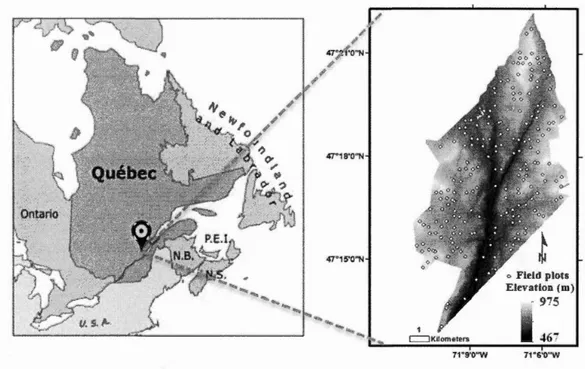
2.4 Study area and data sources ... 30
2.4.1 Study area ... 30
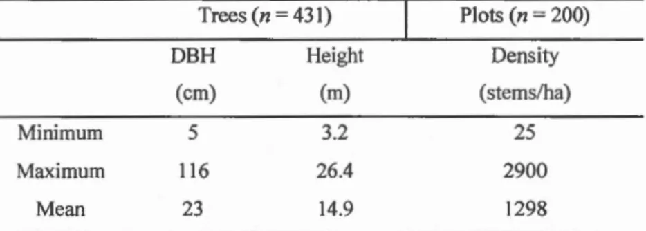
2.4.2 Field and forest in ven tory data ... 31
2.4.3 Remo te sensing data ... 32
2.5 Methods ... 33
2.5.1 Creating the TanDEM-X DSM ... 33
2.5.2 Creating the Lidar DSM ... 34
2.5.3 Creating the DTM and CHMs ... 35
2.5.4 Comparing InSAR and Lidar CHMs ... 36
2.5.5 Relationships between local incidence angle, TanDEM-X ... 39
2.5.6 Effects of forest structure on coherence and dominant ~H ... 39
2.6 Results ... 40
2.7 Discussion ... 58
2.8 Conclusions ... 61
CHAPTER III EFFECTS OF TANDEM-X ACQUISITION PARAMETERS ON THE ACCURACY OF DIGITAL SURFACE MODELS OF A BOREAL FOREST CANOPY ... 65
3.1 Résumé ... 65
3.2 Abstract ... 66
3.3 Introduction ... 67
3.4 Materials ... 71
3.4.1 Study area and field data ... 71
3.4.2 TanDEM-X images ... 73
3.5 Methods ... 75
3.5.1 Creating the DTM, DSMs, and CHMs ... 75
3.5.2 Accuracy assessment of the InSAR CHMs ... 76
3.5.3 Consistency experiment ... 76
3.5.4 Baseline variation experiment.. ... 77
3.5.5 Incidence angle variation experiment ... 77
3.5 .6 Phenol ogy variation experiment ... 77
3.5.7 Analysis of the impact of acquisition conditions on canopy height predictions ... 80
3.6 Results ... 81
3.6.1 Coherence maps and CHMs ... 81
3.6.2 General prediction models ... 87
3. 7 Discussion ... 89
3.8 Conclusions ... 93
CHAPTERIV MAPPING BOREAL FOREST BIOMASS FROM A SRTM AND TANDEM-X BASED CANOPY HEIGHT MODEL AND LANDSAT SPECTRAL INDICES .... 99
4.1 Résumé ... 99
4.2 Abstract ... 96
4.3 Introduction ... 96
· 4.4 Study area and data ... 1 01 4.4.1 Study area ... 101
4.4.2 Reference data ... 102
4.5 Methods ... 1 05 4.5 .1 Calculation of field plot biomass ... 1 05
4.5.2 Creation of li dar biomass maps ... 1 06
4.5.3 SRTM DEM correction ... 106
4.5.4 Creation and validation of the SAR CHM ... 1 10 4.5.5 Biomass prediction from remote sensing variables ... 111
4.6 Results ... 111
4.7 Discussion and conclusion ... 120
CHAPTER V SYNTHESIS, CONCLUSIONS AND FUTURE RESEARCH ... 124
5.1 Scientific contribution ... 125
5.2 Generalization and limitations ... 131
5.3 Future research directions ... 133
5.4 Concluding remarks ... 136
APPENDIXA MAPPING FOREST CANOPY HEIGHT USING TANDEM-X DSM AND AIRBORNE LIDAR DTM ... 138
A.1 Abstract. ... 138
A.2 Introduction ... 139
A.3 Study Site and Data ... 139
A.4 Methodology ... 140
A.5 Results ... 142
A.6 Conclusions ... 145
Figure 2.2 Representation of the two definitions of canopy height ... 35
Figure 2.3 lidar CHM, InSAR CHM, coherence map, and map of the differences between the CHMs ... 42
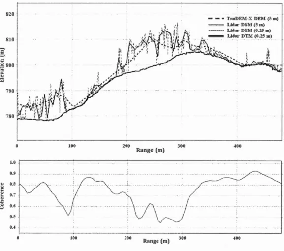
Figure 2.4 The sample profiles of the InSAR DSM, the InSAR CHM ... .43
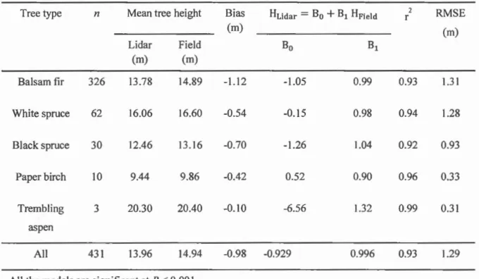
Figure 2.5 lidar vs. field-measured individual tree heights ... .45
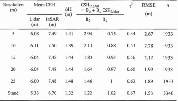
Figure 2.6 Relationships between InSAR and lidar canopy surface height (CSH) .. .47
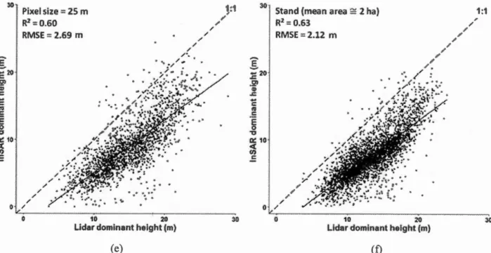
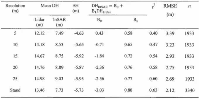
Figure 2.7 Relationships between InSAR DH and lidar DH ... 50
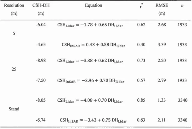
Figure 2.8 Relationships between InSAR CSH and lidar DH ... 52
Figure 2.9 Relationship between a) coherence and local incidence angle, b) 6h and coherence, and c) 6h and local incidenèe angle ... 54
Figure 2.10 Relationships of stem density (a & b), dominant height (DH) (c & d), canopy surface height (CSH) (e & f), and gap volume (g & h) with coherence, and dominant m ... 57
Figure 3.1 Location ofthe Montmorency Research Forest ... 73
Figure 3.2 Coherence maps ... 80
Figure 3.3 InSAR CHM maps ... 81
Figure 3.4 Relationships between InSAR CHMs and the lidar CHM ... 83
Figure 3.5 Relationships between the InSAR CHMs ... 86
Figure 4.1 Location of the study site ... 102
Figure 4.2 SRTM correction process for landform ... 1 09 Figure 4.3 Lidar-predicted vs. Observed biomass for 191 field plots ... 114
Figure 4.4 The height maps for lidar and SAR (20 rn resolution) ... 117
Figure 4.5 Scatterplots of the lidar CHM and the SAR ... 119
Figure 4.6 The relationship between lidar-predicted and SAR-Landsat biomass ... 119
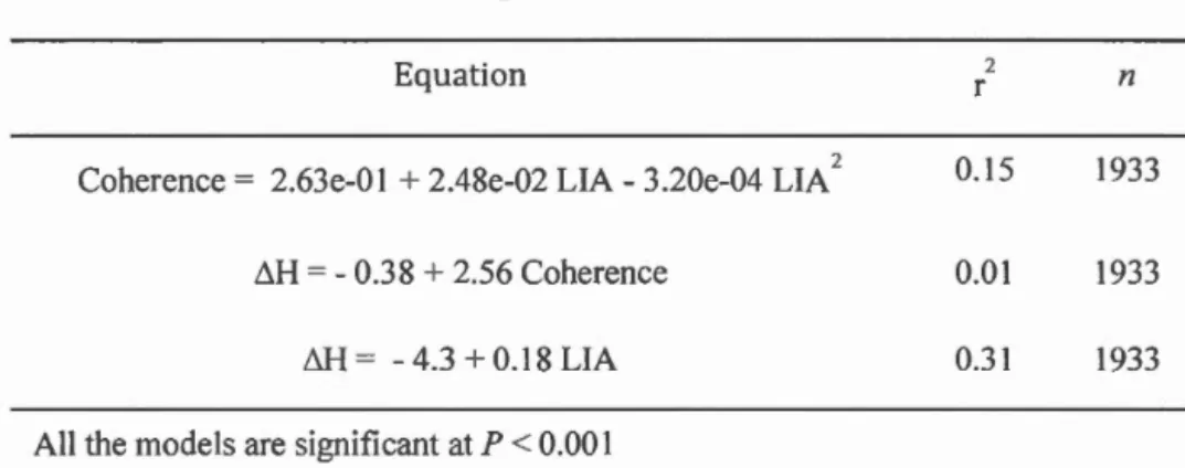
Figure A.l Lidar CHM ... l41 Figure A.2 TanDEM-X-lidar CHM (TanDEM-X DSM minus lidar DTM) ... l42 Figure A.3 TanDEM-X-lidar CHM vs. Lidar CHM ... l43 Figure A.4 Relationship between TanDEM-X InSAR coherence and LIA ... l43 Figure A.5 Relationship between TanDEM-X InSAR coherence and lidar CHM ... 144 Figure A.6 Relationship between InSAR coherence and forest basal area ... 145
Table 2.3 InSAR CSH relationship with the lidar CSH ... .47
Table 2.4 InSAR DH relationship with the lidar OH ... 52
Table 2.5 InSAR CSH and li dar CSH respective relationships to DH ... 53
Table 2.6 Relationships between LIA, coherence, and 6H ... 55
Table 2.7 Relationship between stem density, OH, CSH, gap volume, coherence, .. 58
Table 3.1 The characteristics of tandem-x acquisitions ... 74
Table 3.2 Statistics of the regression between InSAR CHM and lidar CHM ... 84
Table 3.3 Statistics of the comparison experiments ... 87
Table 3.4 General mode! to predict lidar CHM ... 88
Table 3.5 Statistics of the comparison between the predicted and reference CHM using general models (*) ... 89
Table 4.1 General statistics of the main structural attributes of the 200 field plots of the Montmorency Forest ... 103
Table 4.2 Summary characteristics of the remo te sensing data ... 105
Table 4.3 Plot leve] biomass statistics ... 112
Table 4.4 The statistical summary of the SRTM DEMS ... .114
Table 4.5 Statistical between the li dar CHM and the SAR CHM ... 117
Table 4.6 Statistical relationships between SAR-Landsat and lidar predictions of biomass using linear regression and random forest (RF) ... 118
AGL
ATLAS
ALS
AGRG
C02C-CLEAR
CHM
CSHEVI
DBH
DVIDSM
DTM
DHGLAS
DLR
GEDI
GNDVI
Above Ground Leve)
Advanced Topographie Laser Altimeter System
Airborne Laser Scanning
Applied Geomatics Research Group
Carbon Dioxide
Canadian Consortium for lidar Environmental Applications Research
Canopy Height Model
Canopy Surface Height
Enhanced Vegetation Index
Diameter at Breast Height
Difference Vegetation Index
Digital Surface Model
Digital Terrain Mode!
Dominant Height
Geoscience Laser Altimeter System
German Aerospace Centre
Global Ecosystem Dynamics Investigation
GRVI GVI HoA ICESat InSAR
mw
JPL LVIS LAI Lidar LIA MIMI CS MO DIS NGA NSERC NDSI NDVI Poi-InSAR MFFP RF RVoGGreen-Red Vegetation Index Green Vegetation Index
Height of Ambiguity
lee, Cloud, and land Elevation Satellite
Interferometrie Synthetic Aperture Radar
Inverse Distance Weighting
Jet Propulsion Laboratory
Laser Vegetation Imaging Sensor
Leaf Area Index
Light Detection and Ranging
Local Incidence Angle
Michigan Microwave Canopy Scattering Model
Moderate Resolution Imaging Spectroradiometer
National Geospatial-Intelligence Agency
Natural Sciences and Engineering Research Council of Canada
Normalized Difference Snow Index
Normalized Difference Vegetation Index Polarimetric lnterferometry SAR
Québec Ministère des Forêts, de la Faune et des Parcs
Random Forest
RMSE SPC SRTM SNR
ssc
SAVI SAR TanDEM-X 3D TIN Root-Mean-Square Error Scattering Phase CentreShuttle Radar Topographie Mission
Signal to Noise Ratio
Single-look Slant range Complex
Soi! Adjusted Vegetation Index
Synthetic Aperture Radar
TerraSAR-X add-on for Digital Elevation Measurements
Three-dimensional
présentons premièrement des arguments pour préconiser une approche de prédiction de la biomasse à partir de la hauteur de la forêt, plutôt qu'à partir de la réflectance, et nous proposons une logique qui mène à considérer que l'interférométrie radar (InSAR)
spatiale réalisée en une passe est l'une des meilleures approches de cartographie de la
hauteur de la forêt à l'échelle planétaire. Pour cette raison, nous avons utilisé les données des deux seules missions InSAR planétaires à une passe, TanDEM-X et SRTM
(Shuttle Radar Topographie Mission). TanDEM-X, la première et la seule mission
interférométrique globale en bande X, fut amorcée en 2010 et a généré un modèle numérique d'altitude (MNA) planétaire à haute résolution. À travers une comparaison détaillée à des données concomitantes de balayage laser aéroporté (BLA), nous avons d'abord démontré que ce MNA est en fait un modèle numérique de surface (MNS). En
soustrayant de ce MNS un modèle numérique de terrain (MNT) obtenu par BLA, nous
avons pu générer un modèle de hauteur de couvert (MHC). La résolution et l'exactitude de ce MHC InSAR-BLA ont été évaluées à des résolutions allant de 5 rn à 25 rn, et à l'échelle du peuplement forestier. Il fut constaté que ce type de MHC a une résolution inhérente plus grossière que celle d'un MHC correspondant créé par BLA. Son exactitude variait de 2.7 rn (EMQ) à 5 rn de résolution, jusqu'à 1.5 rn à l'échelle du peuplement. Étant donné que les MNS de TanDEM-X sont générés à travers le monde
selon des configurations et en des saisons différentes, nous suspections que cette
variabilité dans les conditions d'acquisition pourrait affecter l'exactitude des MNS de TanDEM-X. Nous avons testé cette hypothèse en évaluant l'exactitude de cinq jeux de données TanDEM-X acquis selon des différentes conditions géométrique et phénologique pour une forêt boréale en majeure partie sempervirente. Les résultats montrent des biais allant de 0.77 rn à 1.56 rn comparativement à des données de BLA, des r2 allant de 0.68 à 0.38, et des EMQ allant de 2.06 rn à 3.67 m. Parmi ces cinq jeux de données TanDEM-X, deux qui furent acquis dans des conditions quasi identiques différaient par 1.27 rn (EMQ), alors que l'effet le plus prononcé provenait d'une large différence de ligne de base interférométrique, menant à une EMQ de 3.27 rn entre les
DSM générés respectivement avec une courte et longue ligne de base
interférométrique. L'effet des changements phénologiques sur les estimations de la hauteur forestière était plus faible que ceux résultant des différences de lignes de base,
avec une EMQ de 2.30 rn entre les jeux de données acquis sans, et avec feuilles (dans
le cas des arbres décidus). Ces résultats indiquent que, malgré des variations dans les
conditions d'acquisition, une mosaïque TanDEM-X continue acquise avec des lignes
de base appropriées pourrait servir à produire des estimations fiables et suffisamment homogènes des altitudes des surfaces des couverts forestiers dans le cas des forêts boréales fermées sempervirentes. Finalement, nous désirions proposer une solution de télédétection pour créer des MHC qui ne dépendrait pas de données de BLA, mais qui
serait plutôt entièrement fondée sur des données acquises par des capteurs satellitaires. Pour cela, nous avons utilisé une méthode de correction des MNA SRTM (acquis en bande C) permettant d'en faire des quasi-MNT. Un MHC InSAR a ensuite été produit par soustraction de ce MNT du MNS TanDEM-X, ce qui a résulté en une EMQ de 2.45 rn, un~ de 0.43 et un biais de 0.07 rn, lorsque comparé aux hauteurs obtenues par BLA à l'échelle du peuplement. Ensuite, un modèle de prédiction de la biomasse basé sur ce MHC ainsi que sur des indices de végétation fut développé. La biomasse forestière a pu ainsi être cartographiée complètement depuis l'espace avec une EMQ de 26 Mg ha-1
, et un~ de 0.62, comparativement à une carte très exacte de la biomasse à l'échelle du peuplement réalisée par BLA. Dans un avenir rapproché, les données SRTM pourraient être remplacées par celles d'une mission en bande L, TanDEM-L, ce qui mènerait à des MNT et MHC améliorés, et ainsi, à de meilleures cartes de biomasse forestière.
Mots-clés: TanDEM-X, modèle de hauteur de couvert (MHC), biomasse, radar interférométrique (InSAR), balayage lidar aéroporté (BLA).
from-height approach to reflectance-based approaches, and propose a rationale for considering spaceborne single-pass interferometrie synthetic aperture radar (InSAR) as being one of the best forest height global mapping approach. For this reason, we have used data from the only two global single-pass InSAR missions, TanDEM-X and SRTM (Shuttle Radar Topographie Mission). TanDEM-X, the first and only global X-band spaceborne single-pass interferometer mission, was launched in 2010 and generated a global digital elevation mode! (DEM) at high-resolution. Through a detailed comparison with concomitant airborne laser scanning (ALS) data, we first demonstrated that this DEM is, in fact, a digital surface model (DSM). By subtracting an ALS DTM (digital terrain mode!) from this surface mode!, we were able to generate a canopy height mode] (CHM). The inherent resolution and accuracy of such InSAR-ALS CHMs were assessed at spatial resolutions ranging from 5 rn to 25 rn, and at forest stand leve!. It was found that this type of CHM has a coarser inherent resolution compared to a corresponding ALS CHM. Its accuracy varied from 2. 7 m (RMSE) at a 5 rn resolution, to 1.5 m at stand leve!. Because TanDEM-X DSMs are generated worldwide using various sensor configurations, and at different seasons, it was suspected that these variable acquisition conditions may affect the accuracy of TanDEM-X DSMs. We tested this hypothesis by assessing the accuracy of five TanDEM-X datasets acquired under various geometrical and phenological conditions over a mostly evergreen boreal forest. The results show biases from 0.77 rn to 1.56 rn compared to ALS data, ~s from 0.68 to 0.38, and RMSEs from 2.06 rn to 3.67 m. Among these five TanDEM-X datasets, two that were acquired in nearly identical conditions differed by 1.27 rn (RMSE) while the strongest effect came from a big difference in the interferometrie baseline, Ieading to a RMSE of3.27 rn between DSMs generated respectively with short and long baselines. The effect of phenological changes on forest height estimations was found weaker than baseline effects, with a RMSE of2.30 m between Ieaf-on and Ieaf-off datasets (in the case of deciduous trees). These results indicate that, despite variations in the acquisition conditions, a continuous TanDEM-X mosaic acquired with proper baselines could produce a reliable and sufficiently homogeneous estimate of canopy surface elevations of evergreen closed-canopy boreal forests. Finally, we wanted to propose a remote sensing solution for creating CHMs that would not rely on ALS data, but rather on data acquired from satellite sensors. For this, we have used a method for correcting the SRTM DEMs (acquired in C-band) to create quasi-DTMs. An InSAR CHM was then produced by subtracting this DTM from a TanDEM-X DSM, resulting in a RMSE of2.45 rn, a~ of 0.43, and a bias of 0.07 m, when compared to ALS heights at stand leve!. Then, a biomass prediction mode! based on this CHM and Landsat vegetation indices was developed. Forest biomass cou id thus be mapped entirely from space with a RMSE of
26 Mg ha-1, and a
.-2
of0.62, compared to a highly accurate ALS biomass map at stand level. ln the near future, the SRTM data could be replaced by that of a planned InSAR satellite mission in L-band, TanDEM-L, leadingto better DTMs and CHMs, and hence, improved forest biomass maps.Key Words: TanDEM-X, canopy height mode! (CHM), biomass, interferometrie synthetic aperture radar (InSAR), airborne laser scanning (ALS).
1.1 Forest biomass mapping importance and requirements
Wh ile the rote of carbon dioxide (C02) in global warming is now ascertained, the fluxes of carbon between the biosphere and the other components of the overall terrestrial system are stiJl being actively studied. Notably, the amount and spatial distribution of carbon stocks stored in forests at any time remain uncertain (Bustamante et al., 2016; Rodriguez-Veiga et al., 2016), and are constantly changing due to growth and disturbances. For example, great amounts of carbon are released into the atmosphere from forested areas as a result of intensive human activities and land cover changes (Gibbs et al., 2007). A number of methods have been developed to monitor forest carbon stocks changes on large scales (Hansen et al., 2003; Lefsky 201 0; Baccini et al., 2012; Saatchi et al., 2011.b; Simard et al., 2011; Thurner et al., 2014), based on the fact that carbon represents half of the biomass of a tree (IPCC 2003). These models rely on spatially explicit data on the dynamics of the above ground biomass (AGB) of the forest, expressed as tons of forest biomass per hectare (Mg ha-1). Therefore, the reduction of the uncertainty of global carbon stocks and fluxes could be achieved through a better assessment of the forest biomass (IPCC 2003).
A general estimation (Houghton et al., 2009), used here as an example, indicates that forest biomass averages 390 Mg ha-1 in tropical forests, 270 Mg ha-1 in temperate forests, and 83 Mg ha-1 in boreal forests. However, large-scale biomass maps of tropical forests, generated with ce li sizes ranging from 500 rn to 1000 rn by different au thors, diverge rather strongly with regards to biomass levels with a standard deviation of the error between Il to 108 Mg ha-1 (Avitabile et al., 2016). The cause ofthis divergence
stems from differences in the methods used, wh ether at the lev el of field measurement
interpolation or scaling up methods, modeling of environmental parameters used as
predictors, or remote sensing techniques (Ometto et al., 2014; Houghton et al., 2001). Therefore, improving the accuracy of forest biomass estimation methods is essential. Furthermore, forests cover very wide areas of the Earth's surface and are rapidly changing, th us using satellite-based remote sensing with global coverage capability and short revisit time is preferable to field or airbome surveys. Fortunately, the number of satellites with the appropriate characteristics for monitoring forests at large scales, such as wavelength, spatial resolution, revisit time, and in sorne cases, interferometrie capability, is increasing. However, this brings the question of selecting the best rem ote sensing data regarding optimal levels of spatial resolution, temporal resolution, and accuracy for producing timely and accurate forest biomass maps. The "optimal" term in this section is directly related to the possibility ofvalidating these maps at specifie resolutions. Availability of precise reference data is the baseline for determining the optimal resolution for the biomass maps.
1.1.1 Optimal spatial resolution of biomass maps
The spatial scales at which forest biomass changes varies between the fine grain level, such as the fall or regrowth of single trees to much coarser levels, such as those at which large fi re events occur (Houghton et al., 20 12; Houghton 201 0). Dynamics such as deforestation, degradation, damage from disease or afforestation occur at various scales. Each of these biomass disturbance factors, separately or in combination with others, can modify biomass from very fine to broad scales (Vanderwel et al., 2013, a&b). Therefore, defining the optimal scale for capturing biomass changes is not immediately evident. ln one instance, a cell size of 100 rn for mapping biomass was suggested, for example, as the optimal spatial resolution because it roughly corresponds to the size of forest stands, which is in an average of one hectare (Houghton et al., 201 2). It was also suggested that: "Global monitoring of forest aboveground biomass
(AGB) with sub-hectare (1 ha= 104 m2) resolution will facilitate the understanding of carbon storageand its flux between forests and the atmosphere (Treuhaft et al., 2015)."
Furthermore, the size of field plots used for the calibration of the statistical models employed in biomass mapping must have a certain size relation to the pixel size of the remote sensing images used. Large differences in the respective sizes of field plots and the corresponding remote sensing pixels increase calibration and validation uncertainties. This problem is complicated by the fact that due to the intensive labor and important costs of establishing each field plot, the need for having a large number ofwell-distributed plots, the size ofthese needs to be kept small. This, in turn, puts a constraint on the cell size of the remote sensing images used for mapping biomass, especially as a large number of permanent small field plots (a few hundreds ofm2 per plot) are already established worldwide and regularly remeasured. Therefore, a rather high spatial resolution (small cell size) should be preferred (Hall et al., 2011; Le Toan et al., 2011; Hurtt et al., 2010; Bergen et al., 2009; Houghton et al., 2009). It follows from this argument that a sensor such as e.g. MO DIS, with a pixel size of250 rn (62 500 m2), cannot be said to have an optimal resolution. However, these MODIS maps, in the case of Canada with its very large areas of forest, could be said to be economically optimal for biomass mapping.
1.1.2 Optimal temporal resolution of biomass maps
Natural disturbances, such as fire, windthrow, insect disease/damage, or human activities causing, or inducing, deforestation as weil as afforestation, affect between 0.2% to 3% ofworld forests annually, i.e. occur at a rather high temporal rate (Hall et al., 2011; Houghton 2005). On the other hand, forest growth, especially in boreal zones, is rather slow, lessening the need for high temporal resolution (short revisit time).
However, inter-seasonal biomass maps would be required to reduce the variability related to forest phenology (leaf-on vs. leaf-off), which can potentially affect the accuracy of forest height or biomass prediction (White et al., 2015; Anderson and Bol stad 20 13). Due to the close relationship between image features or sorne of the ir derivatives, e.g. the normalized difference vegetation index (NDVI) and vegetation phenology (White et al., 2003), image acquisition is often limited to an optimal period. For example, in the northern mixed forests, deciduous trees may bear full, non-senescent leaves during only two to three months per year, while in the tropics; the leaf-on time is between six to nine months (Hall et al., 2011). If an optical sensor (instead of a radar sensor) is being considered, frequent cloudiness brings an additional and severe constraint regarding revisit rate. Moreover, each scene must be sufficiently lit by the sun. ln the case of Landsat 8 for example, day scenes are acquired on descending orbits -while night scenes unusable for biomass studies are taken on ascending orbits. This limits the revisit rate compared to radar sensors which can create scenes of the same are both on ascending and descending orbits. The temporal resolution should, therefore, be high enough in the case or optical imagery to ensure that every location of an area of interest can be seen at !east once in the day time, without clouds, per leaf-on season, which translates into a quasi-daily revisit rate (Asner 2009; Olander et al., 2008).
1.1.3 Optimal accuracy of biomass maps
In a very general way, a biomass prediction mode! can be expressed as:
[1.1]
Where Ê is the biomass predicted using predictors Pi, and E is the random error (unexplained variance). For any resolution cell of a biomass map, the error is the difference between the "true" biomass and Ê.
The first desirable quality of a prediction mode! is that it should not be biased. A significant bias would affect the biomass totals over regions, or biomes, and has, therefore, a great impact on our capacity to assess the real amounts of stored C. In principle, if the mode! is properly calibrated using a representative sample, and weil adapted to the distribution of values (linear, non-linear, etc.), it should not produce biased estimates. However, since the a priori distribution of biomass values, in the ir overall frequencies, or in space, is not known, designing a proper sampling plan over a large area is difficult. Furthermore, access to calibration plots is often arduous in remote areas, leading to a situation where plots are established near access roads (Maltamo et al., 2011 ), which are themselves not randomly distributed in space. In addition, sampling teams may avoid difficult terrains, such as windthrow areas or swamps, and introduce a certain bias (Fisher et al., 2008, Da! ponte et al., 2011 ).
The mode! itself may also be inefficient at producing unbiased prediction over the full range of biomass values. It is weil known (see next section) that models that predict biomass from image reflectance tend to saturate (Lu et al., 20 16) at relatively low biomass levels (1 00-300 Mg ha-1). In this case, the predictions over high biomass areas systematically underestimate the true value.
Random errors, often expressed as root mean square error (RMSE), or %RMSE, have
Jess severe consequences in the case of an unbiased mode! because if these errors are normally distributed around 0, they will cancel out as resolution cells become larger. In general, the smaller the resolution cel! is, the noisier the input signal will be (from, say, remote sensing images), leading to greater RMSE for smaller pixels. This brings us back to the optimal spatial resolution, which can be set such that the highest spatial resolution is preserved, while the RMSE values remain at an acceptable level.
This poses the question of the desired levels of random errors in spatially explicit biomass predictions. First, it should be remembered that field data used to calibrate biomass prediction models are themselves quite uncertain. Indeed, in most cases, the
biomass of trees falling within a plot is obtained by measuring trees in the field, and then using allometric equations to predict their biomass (e.g. Lambert et al., 2005). Many models predict single tree biomass using diameter at breast height (DBH) and height, within species-specific models (Baldasso et al., 2012; Chave et al., 2005; Henry et al., 20 13). Often, the field height measurements are not carried out in full, and are uncertain for tall measured trees, leading to rather uncertain predictions of "field" values that are thereafter used as "reference" for calibration and verification ofremote sensing models. Houghton et al. (2009) report that field-based biomass estimation may have an error of approximately 20% when using allometric equations. We have not found clear accuracy targets in the scientific literature concerning forest biomass estimates. In other carbon modelling domains, researchers report for example an uncertainty of 18% for carbon net uptake by oceans (Canadell et al., 2007). So setting a maximum, or optimal RMSE remains an open question at global scale for biomass estimation.
In summary, the optimal biomass prediction model should be designed such that it requires a smaiJ number of calibration plots, be unbiased, produce undependable predictions over the full range of biomass, and have an acceptable levet of random prediction error at the set resolution. Considering the current state of the art, a 20% RMSE error should not in our opinion be deemed excessive.
1.2 Forest biomass retrieval using spaceborne remote sensing
Satellite remote sensing can be used to estimate forest biomass and monitor its changes on a global scale. Many studies have proposed biomass mapping methods using data from Earth observation satellites, but there is yet no agreement on the best approach. In general, two general families of methods can be identified: 1) reflectance-biomass models, based on a direct relationship between biomass and image reflectance or
backscatter, and 2) forest height-biomass models, where the forest height is used as the main predictor to estimate biomass.
1.2.1 Reflectance-biomass models
Reflectance is the proportion of incident energy that is returned by the forest elements back to the sen sor. In the case of op ti cal sen sors, the energy is sa id to be "reflected," while for radar sensors, it is "backscattered." The proportion of returned energy is determined by geometrie or physical parameters such as vegetation structure, pigments, water contents or its dielectric properties in the case of radar rem ote sensing. Canopy structure (element size and shape, the orientation of leaves or woody stems, surface roughness) will affect the returned energy in both the optical and radar domains. Leaf pigment, namely chlorophyll, and water contents, will affect reflectance in the optical domain. The volumetrie moisture content of canopies will determine their dielectric properties and thus the amount of backscatter microwave energy. Reflectance or backscatter varies depending on wavelength. The short wavelengths of optical sensors (sun's energy in the visible to short wave infrared regions) react to a canopy's small components such as leaves and twigs. They cannot penetrate deeply into the canopy and only return a signal from the surface. They usually carry a signal on the percent cover of canopies, not on the ir height or biomass. Percent cover is the proportion of ground covered by vegetation. For this reason, biomass prediction models based on reflected energy measured using optical sensors tend to saturate at very low levels of biomass (Lu 2006).
Landsat vegetation indices were used for example to estimate forest biomass in the boreal and mixed-conifer forest with a RMSE of 49% (Frazier et al., 2014) and 27% (Pflugmacher et al., 2014), respectively. Optical ASTER spectral information was also used to predict the boreal forest biomass with a RMSE of 41% to 44.7% (Muukkonen
and Heiskanen 2005). By adding texturai indices, Nichol and Sarker (2011) obtained a RMSE of 32 Mg ha-1 using ALOS-A VNIR-2 for estimating forest biomass.
Unlike optical sensors, active radar sensors are not being affected by weather or cloud cover and hence are a good alternative to optical sensors for mapping forest biomass. In this case, due to the physical relationship between backscatter and volumetrie density of canopy elements, the backscatter amplitude information obtained using various polarizations (H and V) or different radar bands are statistically linked to forest biomass. Radar sensors with shorter wavelengths, such as those of the X-band (approximately 3 cm) and C-band (approximately 5 cm) are sensitive to small components of the canopy. The microwave energy at su ch wavelengths is not able to penetrate deeply into the canopy to return a signal relative to biomass from the larger elements of the forest. Longer wavelength microwave in L-band (approximately 24 cm) and P-band (approximately 70 cm) interact with larger forest components, such as branches and stem (Lucas et al., 201 0; Imhoff 1995.a; Imhoff 1995.b; Wang et al., 1995). It has been shown in different studies that the radar backscatter also saturates at certain biomass levels, depending on the wavelength. For example, P-band backscatter saturates at biomass levels of 100 to 300 Mg ha-1 in tropical forest, and 200 Mg ha-1 in the boreal and temperate forests (Saatchi et al., 2011.a; Imhoff 1995.b; Rignot et al., 1995). L-band satu rates at 40 Mg ha-1 to 272 Mg ha-1 (Ahmed et al., 20 14; Saatchi et al., 20 ll.a; Lucas et al., 201 0; lm hoff 1995.b). A biomass saturation leve) of20 Mg ha-1 was observed for the tropical forest using C-band (Imhoff 1995.b). Therefore, models based on reflectance or backscatters are insufficient to cover the full range of the biomass values due to the weak sensitivity to biomass at higher levels. ln the best case, biomass levels up to 300 Mg ha-1 can be estimated, while there are many situations where AGB reaches 600 Mg ha-1
or more in tropical forests. It was even reported that in a Canadian boreal forest field plot (Abitibi region, Quebec), a 400 m2 plot had a biomass more than 600 Mg ha-1 due to the chance concentration of severa) very large
trembling aspens (Benoît St-Onge, pers. comm. 2016). For these reasons, other approaches to biomass estimation from space must be sought.
1.2.2 Forest height-biomass models
Biomass can be conceived as the product oftree volume and tree density. Because the
density of the woody parts oftrees is not highly variable among different species of a
given ecoregion, volume estimations can easily be translated into biomass. The volume of a single tree can, in turn, be sim ply viewed as being proportional to the product of tree width (say, DBH), and tree height. The biomass of a plot, therefore, depends on the number of tree per hectare, their DBH, and height. In closed canopies, during a large part of the growing stage of trees, there indeed exists a very close relationship between canopy height, volume (m3 ha-1) and biomass. Such relationships were weil illustrated in numerous studies based on airborne lidar data (St-Onge et al., 2008.b;
Nresset 2002). Moreover, using remotely sensed height from space as the sole
predictor, Sol berg et al., (2014) estimated boreal forest biomass with a RMSE of 43%.
Lefsky et al. (2002) showed a single equation based on forest height explains 84%
biomass variations for forests in North America and Canada. For this reason, measuring
the height of forest canopies theoretically provides a very useful, albeit imperfect, predictor of biomass.
Forest height as the main predictor of forest biomass can be extracted to sorne extent using satellite-based 3D (three-dimensional) remote sensing (Lindberg et al., 2012;
Hall et al., 2011; Le Toan et al., 2011), and can then be used to estimate wood volume,
which is then converted to biomass, or biomass directly. Spaceborne sensors that acquired 3D data of potential use for forest structural mapping either produce data on sparse sam pies of forest canopies or offer continuous mapping capabilities. The GLAS (Geoscience Laser Altimeter System) sensor is an example of the first category. lt has been used to produce forest vertical profiles within large footprints. Examples of the
other category are radar sensors with interferometry capability. They have been used to generate continuous height maps of either the surface of canopies or sorne intermediate leve! between the canopy surface and ground leve!. Radar sensors have here again an advantage over short wavelength sensors (i.e. using a laser) as they are not impeded by clouds. In the following subsections, we provide details on these different families of 30 spaceborne sensors, and also illustrate how they can be
combined, amongst themselves or with optical image data.
1.2.2.1 Estimating forest height and biomass using the GLAS sensor
The only spaceborne lidar sensor for measuring forest attributes was GLAS. This
instrument was mounted on the lCESat platform (lee, Cloud, and land Elevation
Satellite) as the part of the NASA Earth Observing System (Schutz et al., 2005). lts main mission objective was to help quantify changes in glacier elevations, but it was also used for other applications, such as the extraction of forest height and biomass. GLAS covered most of the Earth 's surface from 86°N to 86° S latitudes from 2003 to 2009. It acquired vertical laser profiles in footprints with a diameter of 65 rn separated by 172 rn along the track, and tracks were ± 1 km apart at the equator. Of course, the acquisition could only be made in clear sky conditions. In the simplest forest cases, i.e. a single-storey dense canopy over the flat horizontal ground, the height of the canopy could be estimated based on the elevation difference between the first intensity peak (canopy surface), and the last one (ground level). However, because of their large footprint, these signais become very ambiguous in the case of sloping terrain or the presence of multi-storey forests. Extracting forest height from GLAS vertical profiles is said to be limited to areas having a slope Jess than 10% (Hilbert and Schmullius
2012). The ICESat platform carrying the GLAS sensor was decommissioned in 201 O.
Despite its inherent limitations, GLAS data was used in attempts to characterize forest height or biomass. Information extracted from the GLAS footprints were extrapolated
using ancillary datasets such as MODIS (Moderate Resolution Imaging
Spectroradiometer) and SRTM (Shuttle Radar Topographie Mission) to produce forest
height maps (Lefsky 201 0; Simard et al., 2011 ). Th en, these forest height maps were
converted to global biomass maps using height-biomass equations adapted to the
different ecoregions. Saatchi et al. (20ll.b) estimated the uncertainty ofthese maps as being of 30%. The main source of error stems from the uncertainty of the forest height derived from GLAS. One global forest height map based on GLAS was evaluated using field height measurements, which resulted in a RMSE of 6.1 rn, and a r2 of 0.5 (Simard etal.,2011).
ICESat-2, carrying the Advanced Topographie Laser Altimeter System (ATLAS) sensor, is set to be launched in 2018. Its laser sensor will use a photon counting technique for reconstructing return waveforms (Markus et al., 20 16; Abdalati et al., 201 0; Brunt et al., 2016). Although the footprint diameter is predicted to be much smaller, at 10 rn, the use of a green laser (532 nm) instead of near infrared in the case
of GLAS (1 064 nm), will generate a much weaker signal over forests due to the
markedly lower reflectance of vegetation in the green relatively to the near infrared.
Applications to forest characterization are not expected to be highly successful based
on the sensor's specifications (Herzfeld et al., 2013).
1.2.2.2 Estimating forest height and biomass using lnSAR
The second type of sensors with spatially continuous mapping ability includes optical
imagers with the stereo capability or radar systems with interferometry capability.
These sensors can provide spatially continuous forest surface elevations or above
ground forest heights mapping and can theoretically yield more accurate results than
the sampling method (Houghton et al., 2007). Optical stereo images, however, suffer
from the same limitations as any other optical imagery sensor, i.e. they cannot acquire
radar-based solutions. Satellite-based interferometrie radar is the only remote sensing
technology that-can guarantee fast acquisition of global and wall-to-wall 3D coverage
without being impeded by cloudiness or limited to daytime. Graham (1974) introduced synthetic aperture radar for topographie mapping. InSAR (interferometrie synthetic aperture radar) was later developed and used on airbome and spacebome sensors in the
1980s and 1990s to generate elevation maps. In InSAR, the phase difference between
two SAR images is calculated and converted into surface elevation differences. These relative elevations can then be converted to absolute values using control points of known elevation. Figure 1.1 presents the interferometrie SAR acquisition geometry. Two sensors separated by a spatial baseline receive signais from which the phase
difference can be measured to produce topographical data.
1 \ 1 \ ~\ \
:e ,
Bj_
1 \ \ \ \'
'
\ \R\
\ \' '
'
1 1 1 1 1 1 1 \ 1 \~118
' 1 \ 1 ,1~
Figure 1.1 Interferometrie SAR acquisition geometry. 1'18 is the difference between the two incidence angles for two sensors,e
is incidence angle of sensor, B is baseline distance between tow sen sors, B 1. is the perpendicular baseline, and Ris the slant range distance.The performance in converting phase to height critically depends on the baseline. The
common term to express the effective spatial basèline is the vertical wavenumber, Kz.
This term can be approximated by equation 1.2. This vertical wavenumber term relates
the interferometrie phase (<p) to the terrain height (h) by equation 1.3. Finally, the terrain height corresponding to the 2rr interferometrie phase change is called the height of ambiguity, or HoA.
K = 2TTBj_
z Rl..sin8 [1.2]
[1.3]
Interferometrie image pairs can be acquired either simultaneously (single-pass) or in two passes (rept?at-pass). The repeat-pass mode is the most common one since it requires just one sensor. However, it is limited to the reconstruction of the topography ofbare lands, or studies of elevation changes, such as land subsidence caused by ground water extraction (Simard et al., 2012).
Minute changes in the forest between two passes suffice to create coherence problems between the two images that preclude interferometrie reconstruction of the canopy elevations. Temporal decorrelation is the main unknown in repeat-pass InSAR systems. It is caused by the motion of forest elements (e.g. branches) due to the wind, as weil as changes in moi sture content or phenological state (fallen leaves, growth, or senescence) (Simard et al., 2012). Temporal decorrelation problems can be solved by using single-pass interferometers, a configuration in which two antennae separated by a certain distance (baseline) are operating simultaneously.
SRTM and TanDEM-X are the only two satellite missions that have acquired data in this mode over the world forests. The SRTM mission (using the C-band principally, with a wavelength of 5.6 cm, and to a lesser extent X-band, at 3.1 cm) operated in
February 2000 with the purpose of generating a global DEM (digital elevation Mode!) of the Barth. The single-pass TanDEM-X mission in X-band (3.1 cm) was put into operation in 2010 with the goal ofproducing a global high-resolution DEM (12 rn) with a relative error of2 rn (completed in 2016).
The instantaneous phase difference allows the calculation of the height of the SPC (Scattering Phase Centre), which in turn is related to the canopy elevation. The vertical location of the SPC relative to the ground surface depends on canopy properties (species, density, foliage, etc.) and radar wavelength. The location of the SPC relative! y to the canopy surface is often referred to as "penetration depth" (Liu et al., 2009; Thirion-Lefevre and Colin-Koeniguer 2007; Balzter et al., 2007.b; lzzawati et al., 2006). For a given forest structure, SPC is closer to the canopy surface at short wavelengths (e.g., in X-band), and deeper within the canopy at longer wavelengths ( e.g., in C- or L-bands ). ln sorne studies, a combination of short and long wavelengths was used to estimate forest height by subtracting the InSAR ground height, based on L-orP-band, from the InSAR canopy surface height obtained in X-band (Balzter et al., 2007.a; Balzter et al., 2007.b; Neeff et al., 2005). Using single polarization, interferometrie SAR can indeed only produce a single height surface such as a DTM or a DSM or something intermediary. Therefore, using two lnSAR systems with short and long wavelengths or a combination of one radar system with the ancillary data su ch as lidar DTM elevations is needed.
In the case of multi-polarization interferometry however, i.e. Pol-InSAR (Polarimetric Interferometrie SAR), techniques can be developed such that data from only one radar system may suffice to estimate forest height (Kugler et al., 2014; Soja et al., 2014; Askne et al., 2013; Praks et al., 2012; Hajnsek et al., 2009). Height can be estimated, for example, by inversion of the RVoG (Random Volume over Ground) mode! (Soja et al., 20 14; Ku gier et al., 20 14; Lee and Fatoyinbo 20 15). Again, a single-pass system,
with multi-polarimetric capabilities, is required for the RVoG or other inversion techniques.
An InSAR height map extracted from TanDEM-X was used to estimate forest volume and biomass by Solberg et al. (2013). It was found that in the studied region a 1 rn forest height increment corresponds to a volume increase of 23 m3 ha-1 and a biomass increase of 14 Mg ha-1 in the boreal forest. The accuracy of this estimation is 43-44% (RMSE) at the plot level, and 19-20% at the stand level. A similar process was applied in managed boreal forests using TanDEM-X InSAR information, and a RMSE of32% for stem volume, and 20% for Lorey's height was achieved (Karila et al., 2015). Moreover, the height of mangroves was estimated with an accuracy of 1 0% using a PollnSAR approach by Lee and Fatoyinbo (20 15).
1.3 The need for combining data from different spaceborne sensors
Using a single spaceborne sensor for mapping biomass is so far not sufficient to extract ali the needed information for producing a global map of forest biomass. Single-pass InSAR sensors offer much promise, but there currently exists only one operational single-pass InSAR mission (TanDEM-X), providing data in dual polarization (HH, VV) only. As will be demonstrated in the next chapter, TanDEM-X interferograms can be used to generate DSMs, not DTMs. The most accurate source ofDTMs is data from ALS, but world coverage is still very patchy. Moreover, InSAR cannot generate data that allows useful species identification, even in very broad classes (such as coniferous vs. deciduous trees). Species information is needed to select the proper height to biomass relationships in the presence of multispecific forests. The combination of InSAR to other remote sensing data therefore necessarily has to be considered.
As explained in section 1.2.2.1, the current existing large-scale forest height and biomass maps have been produced using a combination of GLAS with InSAR and
optical datasets. There is, however, an important limitation to these maps. Forest height
was estimated only within the GLAS footprints, and only in those that did not fall on
stronger slopes. These heights were then averaged per region, each region being
defined by homogeneity criteria, for example in terms of MO DIS spectra. The
GLAS-derived heights are therefore taken as being representative of the average height of each
region. However, there is not guarantee that this is the case. The forest height estimates
are then used as the main predictor ofbiomass. There is a risk that the extrapolation of
the GLAS-derived height to regions creates important errors, including regional or
even global biomass biases.
Ideally, data combination should involve full spatial coverage data, available from
space. Wh ile multispectral optical sensors able to provide sorne information on species
abound, for example, Landsat 8 or Sentine! 2, there is no current spaceborne mission
that could provide a DTM. The closest is the SRTM data, but as we will show with
more details in Chapter IV, the elevations of this dataset are located somewhere
between the ground and the top of the canopy, depending on vegetational
characteristics. As a very promising mission, TanDEM-L should provide a continuous
quasi-DTM worldwide due toits much longer wavelength of23.6 cm that will allow
deep penetration in vegetation (Krieger et al., 2009). This mission from DLR is
however still in its funding stage (Irena Hajnsek, DLR, pers. comm. 2016), and the
earliest launch date is 2023 (DLR-TanDEM-L, 2016).
1 .4 Optimal approach for producing a global biomass map
Based on the considerations presented in the preceding sections, we here define what
is in our opinion the optimal approach for producing a global biomass map. In
• to rely on the height-biomass relationship, and not on a reflectance- or backscatter-biomass relationship;
• full continuous spatial coverage of the world's forests, i.e. approximately from 72°N to 72°S;
• a spatial resolution fine enough (i.e. approx. 20x20 rn or finer) to enable linking field plot data unambiguously to pixels of the remote sensing dataset for calibration and verification purposes;
• the capacity to acquire height data over an entire biome during one fullleaf-on period;
• to achieve biomass predictions with a %RMSE of 20% or better, at the set resolution (e.g. approx. 20x20m);
·Knowing that no spaceborne laser scanner is currently planned, and that stereo imagery is highly impeded by the presence of clouds, the above criteria point towards a single-pass InSAR solution. Ideally, the lnSAR sensors should operate at multiple wavelengths, allowing for the generation of a DSM, and a DTM, from which a global CHM could be developed. They would also be able to acquire data in full polarimetric mode (HH, VV, HV, and VH) at a relatively long wavelength (L or P) to allow the inversion ofmodels such as the RVoG model.
The current spaceborne system with the closest characteristics is TanDEM-X. However, its main, and quite important, limitation is that it cannot provide a DTM (and no other spaceborne sensor can). Interferograms derived from the X-band should represent the elevations of the surface of the canopy because backscattering originates from small components, such as leaves, needles or fine branches (Mougin et al., 1 993). The scattering phase center should, therefore, be at, or just a bit below the top of the canopy. At the on set of this research project (20 11), no one knew exactly where the TanDEM-X SPC would be located vertically, relative to the top of the canopy. It was
also unclear if the polarization mode would affect the location of the SPC. At the IGARSS (International Geoscience and Remote Sensing Symposium) in 2014, the forum where we first presented our results (see Appendix A), the location of the TanDEM-X SPC was still debated and the subject of many questions. These questions are answered in the next chapter, i.e., the first paper composing this thesis.
To map forest height as a predictor, and assuming for the time being that TanDEM-X can provide a global DSM, an accurate DTM is needed. This can only come from an active sensor, such as a lidar or radar sensor, because only those can send pulses that penetrate vegetation canopies, and then obtain a signal from the ground level. For the purpose of the demonstrations that we set out to make within this research project, we first had to recourse to an ALS DTM in order to assess the quality of the TanDEM-X data without introducing uncertaiAty about ground elevation. lt is possible that large land masses will be covered my ALS soon. A current project ("Elevation project," from Natural Resources Canada, Geomatics Canada 2016) exists for creating a unified ALS DTM for the entire southern portion of Canada (approx. south of the 501
h parai lei). Similar projects exist for the United States, Scandinavia, large parts of Europe, etc. However, there does not seem to be any such endeavour in Russia, which contains a large part of boreal forests. The same applies to large parts of Africa and South America, where most tropical forests are found.
For this reason, we have explored, in Chapter IV (3rd thesis paper) the possibility of correcting DEMs from the SRTM mission to create "quasi-DTMs." The penetration of SRTM C-band in vegetation canopies is greater than in X-band but pulses do not reach the ground leve) in dense and tall forest stands. For example, a 12 rn average height difference between SRTM DEM and a lidar DTM was reported by Su et al. (2015). There is, however, evidence that SRTM DEMs can be corrected to a certain degree (Su et al. in 2014 and 2015). Combining the corrected SRTM DEMs with TanDEM-X DSMs could, therefore, be a solution to procure a global CHM at a high-resolution.
From this CHM, forest biomass could be predicted, but the lev el of uncertainty could be higher and remains to be investigated. The DTM would not require frequent updates as the topography does not change rapidly, except following local catastrophic events (e.g. landslides). The DSM would itself require a frequent update, a task that the TanDEM-X mission can accomplish. Fortunately, DLR is already planning a follow-up mission to TanDEM-X (Irena Hajnsek pers. comm. 2016).
1.5 General objective of the research project
ldeally, we would have sought to make the demonstration that the new methods proposed in this thesis for mapping biomass could be applied for any forest in the world, therefore reaching the goal of providing a method for global biomass assessment. This would, however, require current DSMs (from TanDEM-X), DTMs (from lidar) and field datasets in the boreal, temperate, and tropical biomes, as weil as specifie datasets in the sparse savannah or subarctic forests. On the one hand, these resources are expensive and difficult to obtain. On the other, such a broad project exceeds the normal scope of a Ph.D. project and would entait an enormous amou nt of work, better suited for an en tire team of researchers.
We have therefore limited the scope of this project to closed-canopy boreal forests due to location SPC which in these conditions will stay near the top of canopy. Our general objective was to show how TanDEM-X interferograms, when combined to other datasets, can be used to generate height maps which in turn are used to predict and map forest above ground biomass. Throughout this thesis, we test our methods at different resolutions, from 5 rn to stand levet, and assess accuracy at these different resolutions. lt is hoped that our results can be generalized to most closed-canopy boreal forests of the world.
1.6 Specifie objectives and thesis organization
This research thesis is mainly comprised of three papers presenting detailed methods
and results on ali aspects of our doctoral project. The accuracy of digital surface models
extracted from TanDEM-X interferograms, and transformed into CHM by subtracting
a lidar DTM, was evaluated in Chapter II. Due to availability of only HH polarization
of TanDEM-X at global scale, we continued our process based on producing DSM
from HH interferograms. However, the DSM based on VV polarization was extracted
and compared to the HH version, and the differences were found to be negligible. This
assessment was performed at different resolutions from 5 rn to 25 rn pixels and stand lev el. Th en, the effects of various parameters su ch as forest height, forest density, gap volume, and LIA (Local Incidence Angle) on the CHM accuracy were studied.
Because the final DSMs products released by DLR (and distributed commercially by
Airbus Defense and Space) are assembled from interferograms acquired at different
moments in time, under various satellite configurations, we were concemed that they may have variable accuracy in terms ofRMSE and even bias. For this reason, we have studied five DSMs extracted under variable TanDEM-X acquisitions parameters with regard to phenological conditions, interferometrie baseline, and incidence angle. The effect of meteorological conditions was also assessed to a certain degree. The results are presented in the second research paper, i.e. Chapter Ill.
In the following chapter and last thesis paper, we present a method for correcting
SRTM elevations and use the resulting quasi-DTM to generate a CHM by subtracting
its elevations from a TanDEM-X DSM, thus creating a DSM entirely from satellite
sensors. Using this CHM, TanDEM-X interferometrie coherence, and Landsat 8
Finally, Chapter V presents a summary of the results of three thesis papers and
discusses the potential and limitations of the height and biomass maps created, in light
of results obtained by other researchers, and presents future research directions. Our first thesis results were presented in a short paper published in the Proceedings of the IGARSS 2014, in Quebec City. This paper was placed in the appendix section. 1t remains ofinterest despite being Iargely superseded by the papers presented in Chapters II to IV, as it contains earl y and original results, sorne of which do not appear in the journal papers. These results have guided and influenced our research at this early stage.
DSM AND AN AIRBORNE LIDAR DTM IN BOREAL FOREST
This chapter has been published as:
Y. Sadeghi, B. St-Onge, B. Leblon, M. Simard,"Canopy height mode! (CHM) derived
from a TanDEM-X InSAR DSM and an airborne lidar DTM in boreal forest," IEEE J.
Sel. Tapies Appt. Earth Observ. Remote Sens., Vol. 9, issue. 1, pp. 381-397, January 2016.
2.1 Résumé
La mission TanDEM-X, première mission globale d'interferométrie RADAR à passage
unique, permet de générer une cartographie spatialement continue des élévations de la
canopée. Dans cet article, nous évaluons la possibilité d'utiliser les données de TanDEM-X, en combinaison avec un modèle externe numérique de terrain (MNT),
pour cartographier les hauteurs de la canopée en forêt boréale. Une comparaison et la
validation d'un modèle de hauteur de la canopée (MHC) issue des données
TanDEM-X à un MHC de référence lidar a été réalisée sur deux bases comparatives soit: la
hauteur de surface de la canopée (HSC) et la hauteur dominante (HD). Ces comparatifs
ont été réalisés à l'échelle du peuplement à des résolutions spatiales allant de 5 rn à 25 m. La validation du MHC TanDEM-X a permis de démontrer une RMSE de 2.7 rn à
une résolution de 5 rn et de 1.9 rn à une résolution de 25 rn (à l'échelle du peuplement or pour la hauteur moyenne à 1 'échelle du peuplement). Ces résultats nous ont permis de démontrer que le 1\1HC TanDEM-X présentait une résolution plus grossière que le
MHC lidar correspondant. La différence de la hauteur InSAR par rapport à la hauteur
du li dar varie entre 1.2 rn et 1.5 rn, mais les hauteurs InSAR sous-estimaient la hauteur
des arbres dominants de 4.6 m à 7.5 m. Des différences similaires ont été observées
pour les variables HSC et HD TanDEM-X en comparaison au lidar (respectivement
6.04 rn, 8.98 m, et 8.05 rn pour différentes résolutions). Les résultats nous démontrent
que les hauteurs interférométriques TanDEM-X sont très proches de la hauteur de référence de lidar et que la pénétration sous les hauteurs dominantes est causée par la propagation du signal des microondes entre les sommets des arbres et la surface principale du feuillage en forêt boréale. Enfin, la précision des estimations de hauteur
InSAR n'a pas été sensible aux effets de la densité des arbres, mais a été légèrement
affectée par des angles d'incidence locaux, le volume des trouées et la hauteur de la
canopée.
Mot-clés: TanDEM-X modèle de hauteur de la canopée (MHC), lidar MHC, la hauteur
de surface de la canopée (HSC), hauteur dominante (HD)
2.2 Abstract
The first global X-band spaceborne single-pass interferometer mission, TanDEM-X,
provides a spatially-continuous map of global canopy elevations. In this paper we
assess the use ofTanDEM-X data, in corn bi nation with an externat DTM, to map boreal
canopy heights. A comparison of the TanDEM-X CHM to a validated reference li dar CHM was performed based on two definitions of canopy height: canopy surface height
(CSH), and dominant height (DH) at spatial resolutions ranging from 5 rn to 25 m, and
at the stand leve!. We found the TanDEM-X CHM to have a coarser resolution than the corresponding lidar CHM. This was apparent in the height validation of the
TanDEM-X CHM, which had a RMSE of2.7 rn at the 5 rn resolution, 1.9 rn at the 25 rn resolution, and 1.5 rn at the stand lev el. The difference of the InSAR height compared
to the lidar height varied between 1.2 rn and 1.5 rn, but InSAR heights were below the height of dominant trees by 4.6 rn to 7.5 m. Similar discrepancies were observed for the lidar canopy surface height relatively to dominant height (respectively 6.04 rn, 8.98
rn, and 8.05 rn). The results show that the TanDEM-X interferometrie heights are very close to the lidar reference height and that penetration below the dominant height is caused by propagation ofthe microwave signal between the tree apices and the main
foliage surface in the boreal forest. Finally, the accuracy of InSAR height estimates was not sensitive to tree density effects but was moderately affected by local incidence
angles, gap volume, and canopy height.
Keywords: TanDEM-X canopy height model (CHM), lidar CHM, canopy surface
height (CSH), dominant height (DH)
2.3 Introduction
Despite considerable research efforts that have been devoted to developing remote sensing methods for measuring global carbon stocks and fluxes, significant uncertainty
remains in the estimates of carbon that is stored in the Earth's forests (Gonzalez et al.,
2010; Neigh et al., 2013; Hall et al., 2011). Because canopy height is a key parameter
for estimating biomass (Pflugmacher et al., 2008; Dubayah et al., 201 0; Molto et al.,
2014; Feldpausch et al., 2012; Kellner et al., 2009), satellite-based three-dimensional (3D) remote sensing is likely the most efficient and accurate method for quantifying forest biomass globally (Hall et al., 2011; Le Toan et al., 201 1; Lindberg et al., 2012). Two broad types of 3D spacebome sensors exista) low point density, large-footprint li dar (Light Detection and Ranging); and b) imagers such as stereo optical sensors or synthetic aperture radar (SAR). They use two different remote sensing approaches for