Modelling and Reasoning with Software Product Lines with Design Choices

(1)

(2)

Université de Montréal

Modelling and Reasoning with Software Product Lines

with Design Choices

par

Navpreet Kaur

Département d’informatique et de recherche opérationnelle Faculté des arts et des sciences

Mémoire présenté à la Faculté des études supérieures et postdoctorales en vue de l’obtention du grade de

Maître ès sciences (M.Sc.) en Informatique

mars 2019

c

(3)

Sommaire

Les gammes de produits logiciels (Software Product Lines)(SPLs) permettent de gérer la variabilité qui apparaît dans les familles de modèles logiciels connexes en raison des va-riations des besoins des clients. Durant la conception de leurs modifications, les ingénieurs doivent considérer plusieurs conceptions de SPLs alternatives. Cependant, sans informa-tions complètes sur les exigences de qualité souhaitées pour le SPL final, les ingénieurs sont confrontés à une incertitude quant au choix de la conception appropriée. Les formalismes et techniques existants ne conviennent pas à la modélisation et au raisonnement sur l’es-pace à deux dimensions défini par la variabilité et les choix conceptuels. Nous proposons une approche pour modéliser l’incertitude de conception dans les SPLs et, pour analyser et comprendre l’impact des choix conceptuels sur la qualité des SPLs, exprimé comme des propriétés. Nous définissons formellement les Gammes de produits logiciels avec des choix conceptuels (SPLDCs)(Software Product Lines with Design Choices) et nous décrivons une procédure pour les analyser et fournir une rétroaction appropriée aux ingénieurs basée sur l’ordre partiel des catégories de propriétés de SPLDC. Nous illustrons l’applicabilité de notre approche en utilisant un exemple entirément élaboré qui montre le type de rétroactions nuan-cées nécessaire pour des analyses significatives des SPLs en présence de choix conceptuels. Pour évaluer l’évolutivité de notre approche, nous utilisons notre approche sur de nombreux SPLDC et enregistrer des temps d’exécution.

Keywords : Ingénierie de ligne de produit, modélisation, choix de conception, variabilité, incertitude

(4)

Summary

Software product lines (SPLs) allow managing the variability that arises in families of related software models due to varying customer needs. While designing changes to them, engineers need to consider many alternative SPL designs. However, without complete infor-mation about the desired quality requirements of the final SPL, engineers face uncertainty about how to make the appropriate design choices. Existing formalisms and techniques are not well suited to modelling and reasoning about the two dimensional space defined by vari-ability and design choices. We propose an approach for modelling design uncertainty in SPLs and for analyzing and understanding the impact of design choices in the quality of SPLs, expressed as properties. We formally define Software Product Lines with Design Choices (SPLDCs) and outline a procedure for analyzing them and providing appropriate feedback to engineers, based on the partial order of SPLDC property categories. We illustrate the applicability of our approach using a fully worked out example, that shows the kind of nu-anced feedback necessary for meaningful analysis of SPLs in the presence of design choices. To evaluate the scalability of our approach we use our approach over many SPLDCs and record runtimes.

Keywords: Product line engineering, modeling, Design choices, variability, uncertainty

(5)

List of Tables

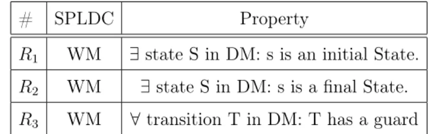
2.1 Quality Requirements for WM example expressed as properties . . . 12

4.1 Levels of satisfaction of SPLDC quality requirements, expressed as properties. . . . 18

4.2 Feedback generated for different property checks . . . 23

6.1 Number of elements in each category . . . 36

6.2 Properties Checked for scalability analysis . . . 36

(9)

List of Figures

1.1 (a) Feature Model, (b) Domain Model of WM SPL . . . 4

1.2 A Variant of WM SPL when features Heat and Delay are selected . . . 5

1.3 (a) Feature Model, (b) Domain Model of WM SPL with design choices . . . 7

2.1 Simplified metamodel of state machines . . . 10

3.1 Choice Model for WM SPLDC . . . 15

6.1 Effect of size of feature model on run time for different sizes of choice model and domain model . . . 37

6.2 Effect of size of choice model on run time for different sizes of feature model and domain model . . . 38

6.3 Effect of size of Domain model on run time for different sizes of choice model and Feature model . . . 39

6.4 Effect of scope on run time . . . 40

(10)

List of Acronyms

API: Application Programming Interface

CM: Choice Model

DM: Domain Model

DSL: Domain Specific Language

EMF: Eclipse Modeling Framework

FM: Feature Model

FOL: First Order Logic

MOF: Meta Object Facility

OMG: Object Management Group

QBF: Quantified Boolean Formula

RQ: Research Question

SAT Solver: Satisfiability Solver

SPL: Software Product Line

SPLDC: Software Product Line with Design Choice

SPLE: Software Product Line Engineering

SPLOT: Software Product Lines Online Tools

UML: Unified Modeling Language

WM: Washing Machine

(11)

Remerciements

I would like to acknowledge my indebtedness and render my warmest thanks to my supervisor, Professor Michalis Famelis, who made this work possible. His friendly guidance, expert advice, and encouragement have been invaluable through all the stages of this work. I also thank him, for providing the Financial Support throughout this period. I have been extremely lucky to have a supervisor who cared so much about my work, and who responded to my questions and queries so promptly. I am thankful to all the Professors and research scholars of the GEODES research group for providing me some useful insights and suggestions about this work and helping me in different ways.

I would like to thank my parents, whose love and guidance are with me in whatever I pursue. They are the ultimate role models. I would like to acknowledge all the hard work they endured for my studies. I am thankful to my brother Arshdeep Singh and his fiance Simrat for all their emotional support and motivation. Furthermore, I wish to thank my caring and supportive friends Joginder Singh, Manvi Virk, Gurpreet Kaur, Khady Fall, Safaa Allamy, Jatinder Singh, and Parminder Kaur for providing an unending inspiration and support.

(12)

Chapter 1

Introduction

The way that industrial products are developed has changed significantly with time. Before the industrial revolution, products were crafted for individual customers. As the number of people able to afford different kinds of products increased, the production line was invented such as the Ford Production line. Production lines facilitate the production for a mass market rather than creating individualized products. This significantly reduced the production cost but at the same time reduced diversification possibilities. Customers were satisfied with standardized mass products for some time – but not everyone wanted the same kind of product, which increased demand to get individualized products. This led to the emergence of the mass customization approach, that is the large-scale development of products designated to individual needs. This meant increased technological expendi-tures, leading to costly products and lower profit margins for the producers. Therefore some companies started to use common platforms for their different kinds of products by antic-ipating in advance which parts will be used in different types of products. This approach enabled producers to offer a greater variety of products and at the same time reduced costs. The amalgamation of mass customization and a common platform allows both the reuse a common base of technology and, to bring out products in close accordance with individual needs [28].

In the case of software products, that already exhibit sprawling complexity, it makes things even more complex while implementing the fusion of the two approaches, as we need to manage the commonality and variability among different software variants. Therefore, there is a need to use some techniques dedicated to this scenario, known as Software Product Line Techniques. For instance, modern cars such as those made by General Motors, can

(13)

contain tens of millions of lines of code, for implementing a variety of functionality such as powertrain control, safety features, climate control, and more. In addition to that, they have to deal with high variability to produce more than 60 models with additional variation to deal with the requirements differences in over 150 countries. To achieve this, they can make extensive use of software product line engineering techniques [14]. Combined with the need to raise the level of abstraction in software development, so that engineers can work using familiar notations, this lead to the emergence of model based techniques. Hence, different model-based techniques are also used by many companies [14].

1.1. Product lines

The need for high degrees of customizability and adaptability in software intensive sys-tems compels developers to create, manage and maintain large families of similar but different product variants. To achieve this, they have at their disposal a wide range of available Soft-ware Product Line (SPL) practices that allow organizations to make long-term commitments to the maintenance of variability in sets of related products [28]. SPLs enables developers to take advantage of the common aspects of products related to each other with some predicted variability. In SPLs, variability is typically modeled using variation points, also known as features, and their inter-dependencies, typically expressed as feature models [31, 28]. Soft-ware product lines can significantly impact many aspects of product development such as: less development and maintenance costs, reduced time-to-market, improved product quality, improved customer satisfaction, reuse of artifacts and more [32]. SPLE techniques have been applied for many years in industries such as automotive, telecommunications, and others.

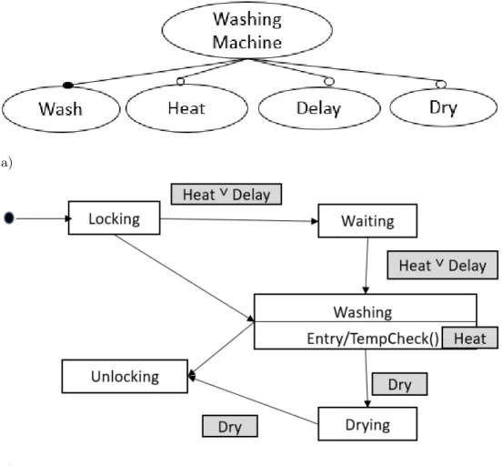
Consider the toy example of a company that develops the software controller for an automated washing system. The company has clients with different needs and has therefore developed a family of products i.e., a family of software controllers called WM. Here we assume that the company uses models to represent its various software artifact [6] We show the WM SPL in Figure 1.1. The WM SPL contains a feature model and a domain model. The feature model has four features: Wash, Heat, Delay and Dry that can be combined to generate several variants. Wash is a mandatory feature, that is, it must be present in all the valid feature configurations, however the other three features are optional. To generate a variant, the developers must select a valid subset of the features of WM. The product variant

(14)

(a)

(b)

Figure 1.1. (a) Feature Model, (b) Domain Model of WM SPL

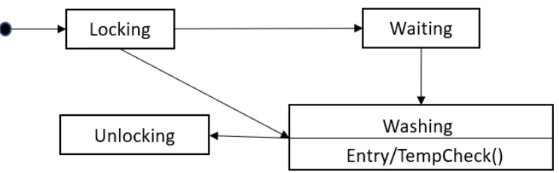
is then generated by appropriately evaluating the presence conditions of the elements of the domain model, shown in Figure 1.1(b) using grey boxes. For example, selecting features Wash, Heat and Delay will generate a variant of the washing machine example which is shown in Figure 1.2. These different combinations of features give different products to the user.

1.2. Design Uncertainty

SPL engineering allows the long-term maintenance of variability options by providing the ability to give individualized products to customers according to their need. However, engineers often need to express and reason about short-term design choices about products. These choices are a source of design uncertainty [29] and can result from many scenarios such as, dealing with different design alternatives, making decisions about product architecture,

(15)

Figure 1.2. A Variant of WM SPL when features Heat and Delay are selected

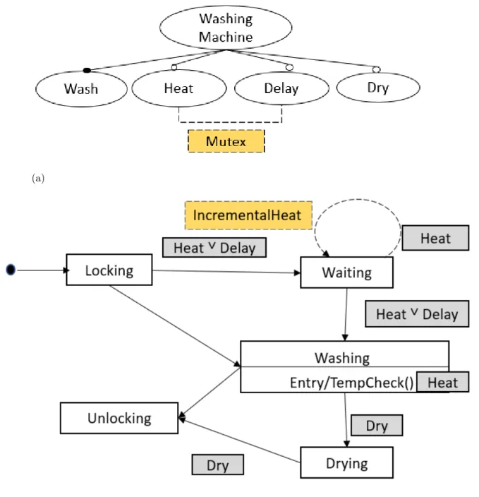
resolving model inconsistencies, or resolving conflicting stakeholder requirements. There can be various design decisions about which developers can be uncertain. Such design decisions can impact various elements of an SPL definition. In our example, while designing the washing machine controller, the developers are not sure if the features Heat and Delay should be mutually exclusive or not. Also, the developers are uncertain if they should provide an option of heating incrementally or not. We represent these uncertainties as boolean design decisions. Each of the two design decisions is shown as a yellow annotation box with dashed outlines on the model elements that are impacted by the decision. Specifically, Mutex is shown as an annotation to the mutual exclusion arc between the Heat and Delay features in Figure1.3(a), and IncrementalHeat as an annotation to a self-transition on the state Waiting, as shown in Figure1.3(b). By answering differently to these design decisions, developers can arrive to different SPL designs. For example, if they decide against Mutex and IncrementalHeat, the resulting SPL is the one shown in Figure 1.1.

1.3. Problem Definition

The design uncertainty implies that there exists a space of possibilities, consisting of the set of product lines that can be created with different combinations of answers to the design choices. These design choices can therefore have significant impact on the quality requirements of the project.

In previous work, it was shown that, instead of finalizing design decisions with little knowledge about their impact, developers can defer making these decisions until they acquire more information [13]. However, that work focused on single products rather than product families. If we consider design uncertainty in product lines then we get the combination

(16)

of both long term variability commitments and short term choices of configurable software designs. We are therefore presented with challenges that cannot be adequately addressed by the state of the art. Suppose, the developers do not have enough knowledge to make the decisions yet, and they want to defer these decisions. But at the same time they want to check some properties of the system, such as consistency. For example, the developers

can check the property R2, shown in Table 2.1, if they want to make sure that whatever

the decision they make in the future, and whatever configuration they choose, the state machine of the resulting controller product will always contain a final state. After analysis, the designers should know whether the system always has this property or not, regardless of the feature configuration they choose and design decisions they make in the future.

Checking these properties is a non trivial task, as both variability and uncertainty are present in the system and must therefore be taken into account in the check. For instance, in the example shown in Figure 1.3, we are uncertain whether the customer wants to have an option to heat for more than one cycle during a load or not. A developer may want to analyze the requirements models, even though they have some uncertainty, to better understand the impact of design decisions on quality. The variability of features and uncertainty among design choices gives a set of software product lines, each of which itself is a set of different products having some commonality. In other words, the analysis must be performed over a powerset of products. However, existing techniques for variability management are not enough for reasoning in this scenario. In [11] Famelis et al. argued that managing the uncertainty induced by design choices is different from managing the variability induced by variation points. The goal of variability management is to support the different variants of a software product line in accordance to different needs among multiple customers. However, uncertainty management provides a means to explore and assess alternative designs, so that software developers can make informed decisions about the design choices [16].

While many approaches exist to manage and reason about variability in product lines [33, 3], and some techniques are developed for uncertainty management [13], there is no signif-icant work to manage both dimensions. This work aims at dealing with the problem of expressing and reasoning about variability and design uncertainty in product lines simul-taneously. In previous work [11] Famelis et al. outlined a research vision for design space exploration for SPLs. In this thesis, we expand on that work, using partial models, defined

(17)

(a)

(b)

Figure 1.3. (a) Feature Model, (b) Domain Model of WM SPL with design choices

in [12], to express decision points. A partial model is a representation of a set of models that could be obtained after resolving the design uncertainty. We call the systems having both decision points and variability points,such that the one in Figure 1.3, Software Product Line with Design Choices (SPLDCs) [11].

(18)

1.4. Research Contribution

The main contributions of this thesis are,

(1) the formal definition of product lines with design choices,

(2) a language for the formal specification of SPLDCs,

(3) a technique to analyze their quality requirements, expressed as structural properties, and

(4) a technique to generate feedback to engineers in the form of counterexample, in case the property is not satisfied for all the categories. We define the different levels of quality requirements of SPLDCs as categories of SPLDC-level properties in [11].

1.5. Thesis Structure

The rest of this document is organized as follows: We describe necessary background on SPL engineering in Chapter 2. In Chapter 3 we introduce the formalism for modelling SPLDCs and in Chapter 4 we describe how to analyze them, while generating appropriate feedback. In Chapter 5 we discuss implementation details of our approach. We discuss related work in Chapter 7 We evaluate the applicability and scalability of SPLDC analysis in Chapter 6 and conclude in Chapter 8.

(19)

Chapter 2

Background

In previous chapter, we explained the basics of product lines. In this chapter, we discuss some terminology related Software Product Line engineering using the annotative product line paradigm [19] and provide formal definition for each term. We also explain the analyzer we use for our approach.

2.1. Software Product Lines

This section provides a formal definition of software product lines.

Définition 2.1.1 (Software Product Lines). A Software Product Line (SPL) S is a 3-tuple < F M, DM, µ > consisting of: a Feature Model FM, a Domain Model DM, and feature mapping µ that maps features to the domain model entities.

For instance, Figure 1.1 represents the SPL of a washing machine controller.

Définition 2.1.2 (Feature Model). A Feature Model F M is a graphical representation of 2-tuple, < F,ΦF > where F is a set of features, and ΦF is a formula representing variability

constraints among them.

There exist various model variants that provide different concrete syntaxes for represent-ing constraints between features [7]. Our work is not dependent on any srepresent-ingle feature model variant; instead we use them merely as a graphical representation of logical constraints [5]. Figure 1(a) represents the feature model of the WM example described above, where Wash, Heat, Delay, and Dry are features, with the constraints that Wash is mandatory which means that, Wash will be present in all valid configurations and other three features are optional.

Each feature uniquely corresponds to a propositional variable. In what follows, we use features and their corresponding variables interchangeably.

(20)

Figure 2.1. Simplified metamodel of state machines

Définition 2.1.3 (Domain Model). A Domain Model DM is a graphical representation of 2-tuple < D, φD > consisting of: a set of various model elements D, and a formula φD that

represents the metamodel and well-formedness constraints.

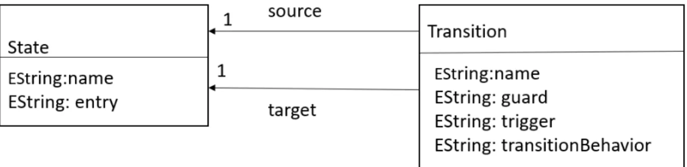
A Domain Model is a representation of entities in the system and relationships between them. The Domain Model can be described using a variety of modelling languages, such as state charts, class diagrams, etc. The domain models for the examples of this thesis are simplified versions of class diagram and state machines. Figure 1(b) depicts the domain model of the WM represented as a state chart. We show the simplified metamodel for state machines in Figure 2.1. For our example, we use state machines that conform to this metamodel. Hence, one of the well-formedness constraint for the domain models represented as state machines is that there is exactly one source for each transition, ∀t : T ransition, ∃s1 :

State · (t = source = s1) ∧ (∃s2 : State · (t.source = s2) ⇒ (s1 = s2)). The formula φD

represents the conjunction of all such constraints.

Définition 2.1.4 (Feature Mapping). A feature mapping µ is a function µ : F M → DM ,

consisting of a set of tuples hE, φEi that map each entity E of the domain model with a

propositional formula φE over the features from the F M . The formulas φE are known as

presence conditions. If we encode the presence of an element e in a product by the proposi-tional variable ve, we can then logically express its feature mapping to the presence condition

φe as Φe = ve ⇔ φe.

We represent presence conditions graphically using grey box annotations next to the

graphical elements that they apply to. In the WM example, the state Drying has the

presence condition φDrying =Dry. This means that state Drying is present in a product iff

the feature Dry is selected.

(21)

2.2. Deriving Products

In this section we discuss the derivation of an individual product from the product line. Définition 2.2.1 (Feature Configuration). A feature configuration ρ of a feature model F M =< F, ΦF > is a subset of features from F that satisfies ΦF. In other words, if in

ΦF we substitute every variable in ρ with true and all others with false, then the resulting

expression evaluates to true. The set of all feature configurations of a feature model F M is denoted by Conf (F M ).

For example, for WM, some of the feature configurations are:

{W ash, Dry}, {W ash, Heat}, {W ash, Delay, Dry}

Définition 2.2.2 (Product Derivation). Given a valid feature configuration ρ, a product M is derived from an SPL, such that only those elements are present in its domain model whose presence conditions are satisfied under ρ. The set of all products that can be derived by a product line SP L is denoted by Conf (SP L)

For example, the WM variant represented in Figure 1.2, is a product derived from SPL using the feature configuration:

ρ = {Wash, Heat, Delay}

2.3. Levels of Property Satisfaction

While analyzing product lines, we can check its properties against different levels of satisfaction. In this section we discuss different levels of property satisfaction for a product line.

Définition 2.3.1 (Product Level Properties). A product level property R is a property that constrains a model without any variability, i.e., properties for individual products, rather than entire SPLs [11].

In this thesis, we focus on structural properties of models. For instance, in the WM example, the property R2 “the model has a final state” is a product level property, which can

(22)

# SPLDC Property

R1 WM ∃ state S in DM: s is an initial State.

R2 WM ∃ state S in DM: s is a final State.

R3 WM ∀ transition T in DM: T has a guard

Table 2.1. Quality Requirements for WM example expressed as properties

be expressed1 _as:

R2 = ∃s : State @t : T ransition · (t.source = s)

The quality requirements for a product are expressed as a set R of product level properties which are desired to be true for that product. The quality requirements for the WM example are shown in Table 2.1.

Generally, we can define the degree of satisfaction of a quality requirement by the number of products of the SPL for which the corresponding property holds. Specifically, we identify two useful levels of satisfaction of a quality requirement:

Définition 2.3.2 (SPL levels of satisfaction). The level of satisfaction of a quality require-ment expressed by a property R of an SPL S is:

A (All): if ∀p ∈ Conf (S) · p |= R. S (Some): if ∃p ∈ Conf (S) · p |= R.

In the WM example the quality requirement that a product always has exactly one final state (property R2) is satisfied by all the products, so its level is A. However, a requirement

that no state has an entry action is clearly not satisfied by any feature that has the Heat feature, therefore, so its level is S.

2.4. Alloy Analyzer

Given the requirements specifications for a system, we sometimes need to check if the property holds for all the models satisfying those requirements or not. This problem is equivalent to proving semantic entailment for first order logic (FOL) which is undecidable. So, rather than checking a property against all the possible models we can extract a relatively

1. To maintain the simplicity of the metamodel of our toy example, we assume that a final state is on that has no outgoing transition. More complex formalisations are of course possible.

(23)

small number of models from given requirements, and check that they satisfy the given property or not [?]. Alloy is a tool that implements this approach. Alloy is typically used for describing the structures and it is supported by the Alloy Analyzer, a tool for exploring those structures [17]. Alloy avoids the problem of the undecidability of FOL by putting a finite bound on the size of models, and check whether the property is satisfied by all the models whose size falls within the given bound and that satisfy all the requirements. We refer to this bound also as a “scope”. A positive result to the check indicates that the property is valid for all models that come within the scope. The result is a proof only within the scope. There is no guarantee for larger models. However, a positive result provides us some confidence. To gain more confidence, we can increase the bound a little further. The negative response, on the other hand, is conclusive. It tells us that there exists at least one model that does not satisfy the property. Alloy is based on D. Jackson’s small cope hypothesis, which states that negative answers tend to occur in small models already [?]. This allows us to assume that we can reach useful conclusions in small scopes, even if we cannot provide general proofs.

(24)

Chapter 3

Modelling Design Choices

In this chapter we describe the way in which design choices can be modelled in product lines.

3.1. SPLDCs

Design uncertainty can affect any part of a product line definition for which modellers need to make a design decision. This includes uncertainty in the design of the domain model (like the choice IncrementalHeat in WM), of the feature model (like the choice Mutex in WM) or of the feature mapping. Famelis et al. introduced partial models as a formalism to represent design uncertainty [15], as well as different variants of partial models [30], that can express more complex types of partiality. In this thesis, we make two key assumptions:

(1) that modellers are aware of the design choices about the SPL that need to be addressed in the short term, and

(2) that for each such choice, a set of possible acceptable solutions has been elicited.

Design choices can therefore be represented as boolean choice variables.

Définition 3.1.1 (Design choice). A design choice is a propositional variable that encodes the choice of a particular solution to a design problem.

So as long as a design choice variable is not bound to True or False, it represents the modeller’s uncertainty about that choice. For example, the design choice Mutex is a propo-sitional variable encoding the uncertainty that modellers have whether the features Heat and Delay should be mutually exclusive.

To represent potential dependencies between design choices, we use a special feature model, called a “choice model”:

(25)

Figure 3.1. Choice Model for WM SPLDC

Définition 3.1.2 (Choice Model). A choice model CM , is a graphical representation of a tuple < C, φC >, where C is a set of design choices C, and φC a formula representing

dependencies between them.

For example, the choice model for WM, drawn as a feature diagram, is shown in Fig-ure 3.1. It consists of the two optional decisions Mutex and IncrementalHeat. Same as in Section 2.1, we do not assert any particular feature model dialect. We simply assume that the FM and CM are both expressed in the same dialect.

The design choices that capture the design uncertainty of modellers about an SPL, can then be mapped to the SPL elements as follows:

Définition 3.1.3 (Decision Mapping). A decision mapping δ is a function δ : CM → SP L consisting of a set of tuples < S, φS >, mapping each entity S of an SPL to a propositional

formula φS defined over the SPL entities with respect to the choices in CM . If we encode

the presence of an element s in an SPL design by the propositional variable vs, we can then

logically express its decision mapping to φs as Φs = vs ⇔ φs.

For instance, in WM shown in Figure 1.3(b) the transition looping over state Waiting is present in a product iff the choice IncrementalHeat is selected.

Using the above definitions, we can therefore formally define an SPLDC as:

Définition 3.1.4 (Software Product Line with Design Choices (SPLDC)). An SPLDC is a tuple hCM, SP L, δi where SPL is a product line definition, CM is a choice model and δ is the decision mapping between them.

For instance, Figure 1.3 represents an SPLDC of WM controller, where yellow boxes represent the design choices Mutex and IncrementalHeat.

The SPLDC allows representing both long term configuration options (in the FM of the underlying SPL definition) and short term design choices for which the developers have uncertainty (in the CM). If developers acquire information that allows them to resolve this uncertainty, they can make decisions about the design choices.

(26)

3.2. Deriving SPLs

Définition 3.2.1 (Design Decision). Given the choice model CM =< C, φC > of an SPLDC

SC, a valid design decision α is a subset of design choice variables from C that satisfy φC.

In other words, if in φC we substitute all variables in α by true and all other variables by

false, the resulting expression evaluates to true. The set of all valid design decisions of SC is denoted as Ch(SC).

In the WM example we have that: Ch(WM) ={ { }, {Mutex, IncrementalHeat}, {Mutex}, {IncrementalHeat}}.

Given the previous definitions, the concretization of an SPLDCs is defined thus:

Définition 3.2.2 (Concretization). A concretization n of an SPLDC S = hCM,S,δi is an SPL that can be derived from S under a design decision α, such that it contains only elements of S that are mapped by δ under α. A concretization is a model without design uncertainty that results from resolving all design uncertainty in a partial model [15]. The set of all concretizations that can be derived from S is denoted by Ch(S).

For example the SPL shown in Figure 1.1 is a concretization of the WM SPLDC that can be derived using the decision α = {}.

(27)

Chapter 4

Reasoning about SPLDCs

In this chapter we propose an approach to reason about the properties of SPLDCs. We discuss the various satisfaction levels for SPLDC quality requirements, expressed as properties. We provide an analysis procedure for analyzing the properties of SPLDCs and show its correctness.

4.1. Levels of SPLDC properties

Similar to the degree of satisfaction of a quality requirement by an SPL in Definition 2.3.2, we can define the degree of satisfaction of a quality requirement by an SPLDC, as the number of SPLs and number of products of an SPL, for which the corresponding property holds. Specifically, we identify four useful levels of satisfaction of a quality requirements:

Définition 4.1.1 (SPLDC levels of satisfaction). The level of satisfaction of a quality re-quirement expressed by a property R of an SPLDC SC is:

N A (Necessary All): if ∀s ∈ Ch(SC), ∀p ∈ Conf (s) · p |= R N S (Necessary Some): if ∀s ∈ Ch(SC), ∃p ∈ Conf (s) · p |= R PA (Possible All): if ∃s ∈ Ch(SC), ∀p ∈ Conf (s) · p |= R PS (Possible Some): if ∃s ∈ Ch(SC), ∃p ∈ Conf (s) · p |= R

For example, for the property R2 given in Table 6.2 with respect to any SPLDC, the

different levels have the following meaning:

N A : Regardless what decisions are made to create an SPL, every possible configuration will lead to a state machine with final state.

(28)

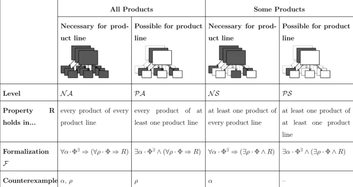
Table 4.1. Levels of satisfaction of SPLDC quality requirements, expressed as properties.

All Products Some Products

Necessary for prod-uct line

Possible for product line

Necessary for prod-uct line

Possible for product line

Pn

Level N A PA N S PS

Property R holds in...

every product of every product line

every product of at least one product line

at least one product of every product line

at least one product of at least one product line

Formalization F

∀α · Φ∃_{⇒ (∀ρ · Φ ⇒ R) ∃α · Φ}∃_{∧ (∀ρ · Φ ⇒ R)} _{∀α · Φ}∃_{⇒ (∃ρ · Φ ∧ R)} _{∃α · Φ}∃_{∧ (∃ρ · Φ ∧ R)}

Counterexample α, ρ ρ α –

N S : There is a set of design decisions that would lead to an SPL design for which every possible configuration will lead to a state machine with final state.

PA : Regardless what decisions are made, it is always possible to configure the resulting SPL such that a state machine can be derived with final state.

PS : There is a set of design decisions that would lead to an SPL design which is possible to configure to derive a state machine with final state.

We summarize the four levels in Table 4.1.

Using logical consequence as a binary relation between levels, the four levels form a partially ordered set (poset ), where PS is the minimal and N A is the maximal element, and where N S and PA are at same rank. In other words, if for example for an SPL S, a property R is satisfied at level N A, it is also satisfied at levels, PA, N S, and PS, while if it is satisfied at level PA or N S it is also satisfied at level PS. Conversely, if the property is not satisfied for level PS, it is not satisfied for any other level, etc. More formally, we observe that given the lemma of Bjorner [2] that a bounded poset of finite rank forms a lattice, the four SPLDC requirement satisfaction levels form the lattice:

In the following, we denote this lattice as L.

(29)

N A

N S PA

PS

4.2. Analysis procedure

Given this observation, we can define an analysis procedure for SPLDC properties, which we illustrate with the WM example. We assume as inputs the specification of an SPLDC K according to Definition 3.1.4, as well as a quality requirement R expressed as a first order logic property. Our aim is to understand the level of satisfaction of R in K.

First, we encode the SPLDC K in logic. Specifically, we construct the formula:

Φ = ΦF ∧ ΦD ∧ ^ e∈E Φe∧ ΦC∧ ^ s∈S Φs

Where ΦF is given in Definition 2.1.2, ΦD in Definition 2.1.3, the set of formulas Φe over

the set E of Domain Model elements in Definition 2.1.4, ΦC in Definition 3.1.2, and the

set of formulas Φs over the set S of elements of the SPL (features, domain model elements

and feature mapping tuples) in Definition 3.1.3. The formula Φ encodes the entire two dimensional space of SPLs and products; a valid design decision α and a valid configuration ρ define exactly one satisfying assignment for it.

To check if a property is satisfied at a particular level, we check the validity of the corre-sponding logical formalization F of that level, according to Table 4.1, using a satisfiability checker such as Sat4J [21]. The formulas FN A,FPA,FN S, and FPS were first introduced in

[11] but in this thesis we integrate them in a coherent modelling and analysis approach. In effect they lift product-level properties to the SPLDC level, allowing the quantification over design choices and features. We describe their construction below.

The formula Φ is satisfied for combinations of decision and feature variables. However, when reasoning about SPLDCs, we want to be able to provide nuanced feedback to users, separating the cause of analysis results into each dimension. We therefore use the formula Φ∃ which encodes the dependency constraints on just the design choice variables; it is derived from Φ by quantifying out [36] all variables except for those representing design choices. This allows us to separate quantification over design choice and feature variables. Each combination of values assigned to the design choice variables is a design decision α, i.e.,

(30)

a set of decisions in the design space that define a single SPL design. Each subsequent combination of feature variables is a product configuration ρ of that SPL design.

In case a quality requirement is not satisfied at a particular level, we produce appropriate feedback by using the counterexample generated by the satisfiability checker during the validity check. This consists of a truth assignment of the design choice variables in α and/or the feature variables in ρ depending on the level, see Table 4.1. We translate this truth assignment back to the level of abstraction used for SPLDC modelling and present it to the user as a counterexample. There is an obvious tradeoff between generating nuanced feedback that separates between the two dimensions (variability and design choices). The computation requires the existential quantification over the two different sets of variables and the check for satisfiability, and is therefore computationally costly.

To analyse the overall level of satisfaction of a requirement R, we start our analysis at

the maximal element of L, and move downwards. At rank 2, the order of checking FPA and

FN S is irrelevant. In the worst case (where the property is not satisfied by any product of

any possible product line design), four checks are required in total.

Suppose we want to analyze requirement property R1 (“there is an initial state”) given in

Table 2.1, that is expressed by the formula R1 = ∃s : State @t : T ransition · (t.target = s).

First we check whether its level of satisfaction is N A. To do this, we construct FN A using

the logical encoding of the WM SPLDC and R1, and check whether it is valid, using a

satisfiability checker. We find that it is, and therefore we neither need to check the other levels, nor to produce any further feedback to the modellers.

Suppose that we then want to analyze the property R3 (“there exists a transition that has

a guard”) from Table 2.1. Following the same process, we find that it is not satisfied for N A. To help modellers understand why, we pinpoint a product that violates the property, by providing a set of design and configuration choices. The exact choice of feedback depends on the satisfiability solver, but one possibility is α={Mutex} and ρ={Wash,Dry}. Going down the lattice L, we check whether R3 is satisfied for level N S, also getting a counterexample.

In this case, the counterexample is a design decision α that results in an SPL concretization with no products that satisfy the property. A possible feedback generated by the solver is α={Mutex,IncrementalHeat} as resulting the SPL has no product that contains a

transition with a guard. We also check whether R3 is satisfied for level PA, which also

(31)

generates as a counterexample a configuration that exists in every product line and for which the property is not satisfied. A possible feedback generated by the solver is ρ={Wash}: the simplest washing machine configuration is included in all SPL concretizations and does not contain any transitions with guards. Finally, we check the lowest level of L, i.e., whether

R3 is satisfied at level PS. We find that it is not (obviously, as the domain model of WM,

shown in Figure 1.3(b), does not contain any guards to begin with) and the solver does not need to generate a counterexample, as by definition every combination of α and ρ is a counterexample.

4.2.1. Correctness

Using the appropriate formalization formula F from Table 4.1, we can prove whether a property R of an SPLDC K is satisfied at the corresponding level, per Definition 4.1.1. Below, we state this as a theorem for level N A. The theorems and proofs for levels PA, N S, and PS are analogous.

Théorème 4.2.1. Given an SPLDC K, encoded logically as Φ, and a quality requirement

R of K, expressed as a property, the level of satisfaction of R is N A iff the formula FN A

(R)= ∀α · Φ∃ ⇒ (∀ρ · Φ ⇒ R) is valid.

Proof. The satisfaction level of R in K is N A if ∀s ∈ Ch(K), ∀p ∈ Conf (s) · p |= R. Assume that there is an SPL concretization s in Ch(K) from which we can derive a product

p in Conf (s) such that p 6|= R. That means that there is a design decision αs that can be

used to derive s from K and that there is a configuration ρp that can be used to derive p

from s. But since the formula FN A (R) is valid, it is true for every design decision α and

configuration ρ. Therefore there is no way to derive a p such that p 6|= R and thus the satisfaction level of R for K is N A.

Conversely, if the level of R in K is N A, then for every s in Ch(K), i.e., for every decision αs, every product p in Conf (s), i.e., for every configuration ρp, it is the case that p |= R.

(32)

4.3. Illustration

4.3.1. Setup

We illustrated our approach, to know about the kinds of insights we gain from the prop-erty analysis of SPLDCs. To do so, we transformed the counterexamples produced by Alloy for various property checks, to our domain specific languageTyson discussed in Chapter 5. The transformed counterexamples contain the feature configuration, choice configuration, or both, of the product or the product line that does not satisfy the property for a given level. The type of feedback given for each level of property check is described in the last row of Table 4.1.

— If a property fails to satisfy level N A, then it could be because of the feature configu-ration or the design choices that are made for the product for which the property fails. Therefore, we provide both feature configuration of the product and design decision of the product line containing that product for counterexample at level N S.

— If the property fails at level N S, then the possible reason for not satisfying the property is the design decision made for the SPL that fails to satisfy the property. So, for the counterexamples at level N S we give the design decision for the product line where the property is violated.

— For properties that do not satisfy level PA, we provide the feature configuration for the product that violates the property.

— If the property is not satisfied for level PS then there is no product in SPLDC that satisfies the property. We do not provide any feedback for this level because the violation of the property is caused by the entities that are always present in the models. In other words, it is not caused because of a particular design decision or a feature configuration.

Based on the feedback we provide for each level, the developer can make sure not to make the design decisions or choose the feature configuration that does not satisfy the property. Developers can also add constraints to make sure that a particular feature configuration or design decision is never present in the system.

We use the WM example described in Chapter 1. The WM example is inspired from the motivating example in [11]. We used a slightly different version of the example in [11] to add

(33)

# Property Result Counterexample Decision Counterexample Configuration 1 ∃ state S in DM: s is initial State.

SAT for all levels -

-2 ∃ state S in DM: s is Final State.

SAT for all levels -

-3 ∃ Transition T: t.source = t.target

Violates level N S IncrementalHeat

-4 ∃ Transition T:

t.target=waiting

Violates level PS - Wash, Dry

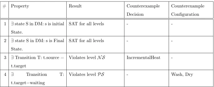
Table 4.2. Feedback generated for different property checks

another design choice to the example. The example is then represented in Alloy specification language [17], and the properties we want to analyze are written as Alloy Assertions.

4.3.2. Observations

We analyze the WM example against 4 properties. The feedback generated for each property check on WM is shown in Table 4.2. Two of these properties satisfy level N A which means that they satisfy all levels of property satisfaction. The property that checks there is no self loop in the state chart, fails at level N S, so the feedback generated gives the decision Incremental Heat Fourth property checks if waiting is always present in system. The satisfaction level for this property is PA, the feedback gives a feature configuration { Wash, Dry}

4.3.3. Discussion

The feedback we provide gives an insight to the developers about the issues present in the system. It gives the possible reason behind the violation of a property. To raise the sat-isfaction level for a property, the developers can make changes in accordance to the feedback provided. For instance, for Property #3 in the Table 4.2, we get the counterexample at level N S, which gives contains the design decision IncrementalHeat. The result implies that the possible reason behind the non-satisfiability is the presence of decision IncrementalHeat.

(34)

So, to improve the level of satisfiability, the developer can decide against IncrementalHeat and check the property again.

Our study shows that the feedback generated for the property check, provides insights about the models that can help in improvement of a certain property satisfaction level. This gives us initial evidence for the usefulness and applicability of the study, giving us confidence to do further research on the topic.

We illustrated our approach on a small, synthetic example. However, despite its size, the example is enough to showcase that we can generate feedback that is useful in terms of helping modellers plan their responses to property violations. Furthermore, we are currently planning a bigger case study from the domain of mixed-criticality cyber-physical systems.

(35)

Chapter 5

Implementing SPLDCs in Tyson

In this Chapter we discuss the implementation of the approach discussed in Chapter 4. We have developed a Domain Specific Language (DSL), called Tyson, to simultaneously express variability and design uncertainty. In the following, we use the WM example to illustrate how Tyson can be used to model SPLDCs. The full Tyson specification of the WM example can be found in Appendix B.1

5.1. Language Basics

In order to specify SPLDCs, we need a language that can represent different entities of SPLDCs, and mapping among them. To accomplish this, we developed a textual language called Tyson. Tyson is a textual language developed using Xtext, a framework for the creation of programming languages and DSLs [10].

Xtext facilitates the development of DSLs by allowing the creation of a full infrastruc-ture stack that includes a parser, linker, type checker, compiler, and editor with syntax highlighting. Xtext automatically generates an ecore metamodel for the language based on the grammar we write. Ecore is the core eclipse modeling framework (EMF), which allows us to describe models and provide run time support for the models. Ecore is an efficient API for generically manipulating EMF objects [8].

Tyson is specifically designed to express SPLDCs. The metamodel for Tyson is shown in the Appendix A.1. We can declare 3 kinds of models in Tyson: 1) a feature model that represent all the features and constraints among them, 2) a choice model that represents all the design choices the developer is uncertain about and, constraints among them, 3) domain model of the system. Apart from representing all different entities of SPLDCs, we

(36)

also need to represent relations among them. We represent these relations in terms of two kinds of mappings: 1) Feature Mappings, which represent how features impact the presence of domain model entities 2) Decision Mappings, which represent how the different design choices impact product line entities. The Listing 5.1 shows the definition of choice model in Tyson having two design choices as described in Chapter 1.

Listing 5.1. Choice Model Definition in Tyson

CM { Mutex ;

I n c r e m e n t a l H e a t ;

}

Listing 5.2 shows the definition of Feature Model shown in Figure 1.3(a) having 4 fea-tures. We also define a constraint that Wash is a Mandatory feature. Tyson also allows the definition of multiplicity constraints about a feature group. Similarly, we can also define constraints about design choices as a part of choice model definition.

Listing 5.2. Feature Model Definition in Tyson

FM { Wash ;

Delay ;

Dry ; Heat ;

FMConst:[ Mandatory(Wash) ] }

Listing 5.3 defines the domain model shown in Figure 1.3(b) in Tyson having 5 states and 7 Transitions: T1, T2, T3, T4, T5, T6, T7. In this example the domain model is a State Chart. Tyson currently supports DMs conforming to simplified State Chart and UML Class Diagram metamodels.

Listing 5.3. Domain Model Definition in Tyson

StateChart{

State L o c k i n g ; State Waiting ;

(37)

State Washing ; State Drying ;

State UnLocking ;

Transition T1 : L o c k i n g t o Waiting

Transition T2 : Waiting t o Washing

Transition T3 : L o c k i n g t o Washing

Transition T4 : Washing t o UnLocking

Transition T5 : Washing t o Drying Transition T6 : Drying t o UnLocking

Transition T7 : Waiting t o Waiting }

Mappings among various entities of SPLDC are shown in Listing 5.4. F1, F2, and F3 are Feature Mappings, that represent how the presence or absence of a feature effects the entities of domain model. F1 shows that presence of Wash in Feature Model implies that Transition T2 and T5 are present in Domain model; otherwise they will be absent. D1 and D2 are Decision Mappings, that represents how the presence or absence of design choices can impact the product line entities. D1 shows that presence of Design Choice Mutex implies that presence of Features Heat and Delay are mutually exclusive; its absence that they are not.

Listing 5.4. Mappings among SPLDC entities in Tyson

Mappings {

FMap {

F1: { (Wash IN ) =>

AND (Transition T3 IN , Transition T4 IN ) }

F2 : {OR ( Heat IN , Delay IN ) =>

AND (Transition T1 IN , Transition T2 IN ) }

F3 : { ( Dry 2IN ) =>

(38)

DMap {

D1 : {Mutex IN =>

XOR (Feature Heat IN , Feature Delay IN ) }

D2 : { I n c r e m e n t a l H e a t IN =>

Transition T7 IN }} }

5.2. Tyson Semantics

The purpose of representing SPLDCs is to analyze and reason about their various prop-erties. Therefore, we need to provide semantics to Tyson, that can facilitate the analysis of SPLDCs. To achieve this task, the Tyson models are transformed into Alloy. Alloy is a a lightweight formal method which allows us to do a bounded reasoning of first order logic. Alloy uses the Kodkod model finder and can leverage a variety of SAT solvers used as block box reasoners.

These SAT Solvers allow us to analyze different properties of the system written as assertions. To analyze SPLDCs, Tyson models are transformed into Alloy. We used Acceleo templates to do this transformation. Acceleo is a pragmatic implementation of the OMG MOF Model to Text standard [27]. In other words, we used an Acceleo transformation to give semantics to Tyson via a translation to a formal language: Alloy. Acceleo takes the models represented in Tyson and convert them as text that corresponds to Alloy Specifications for the Tyson models. The full Acceleo translation is provided in Appendix D.1 The full Alloy semantics of the WM example is provided in Appendix C.1.

Tyson does not provide a property specification language; instead, SPLDC properties are written directly in Alloy. In Section 5.3, we show how such properties can be checked for the 4 satisfaction levels in L.

The Listing 5.5 represents the choice model definition in Alloy for the choice model in Listing 5.1.

Listing 5.5. Choice Model Definition in Alloy

a b s t r a c t sig C h o i c e {}

sig Mutex , I n c r e m e n t a l H e a t e x t e n d s C h o i c e {}

(39)

// C h o i c e M o d e l d e f i n i t i o n a b s t r a c t sig C h o i c e M o d e l { c h o i c e : set C h o i c e }

Using Acceleo, the Feature Model defined in listing 5.2, will be transformed to the code represented in Listing 5.6. The Fact written in the code represents the constraint about feature Wash.

Listing 5.6. Feature Model Definition in Alloy

a b s t r a c t sig F e a t u r e {}

one sig Wash , H e a t , Delay , Dry e x t e n d s F e a t u r e {}

a b s t r a c t sig F e a t u r e M o d e l { f e a t u r e: s o m e F e a t u r e } f a c t { all f: F e a t u r e M o d e l | W a s h in f . f e a t u r e }

Listing 5.3 which defines the domain model in Tyson, is transformed as Listing 5.7 in Alloy. The metamodel well-formedness constraint states that if a transition is present in a Domain Model, then its source state and target states will also be present in the Domain Model.

Listing 5.7. Domain Model Definition in Alloy

a b s t r a c t sig S t a t e {}

one sig Locking , Waiting , Washing , Drying , U n l o c k i n g e x t e n d s S t a t e {}

a b s t r a c t sig T r a n s i t i o n { s o u r c e: one State , t a r g e t: one S t a t e }

(40)

f a c t {( T1 . s o u r c e = L o c k i n g ) and ( T1 . t a r g e t = W a i t i n g ) } f a c t {( T2 . s o u r c e = W a i t i n g ) and ( T2 . t a r g e t = W a s h i n g ) } f a c t {( T3 . s o u r c e = L o c k i n g ) and ( T3 . t a r g e t = W a s h i n g ) } f a c t {( T4 . s o u r c e = W a s h i n g ) and ( T4 . t a r g e t = U n l o c k i n g ) } f a c t {( T5 . s o u r c e = W a s h i n g ) and ( T5 . t a r g e t = D r y i n g ) } f a c t {( T6 . s o u r c e = D r y i n g ) and ( T6 . t a r g e t = U n l o c k i n g ) } f a c t {( T7 . s o u r c e = W a i t i n g ) and ( T7 . t a r g e t = W a i t i n g ) } // D O M A I N M O D E L D E F I N I T I O N // c o n t a i n e r for m o d e l el e m e n t s , i . e . , the d o m a i n m o d e l sig D o m a i n M o d e l { t r a n s i t i o n: s o m e T r a n s i t i o n , s t a t e: s o m e S t a t e } // M e t a m o d e l well - f o r m e d n e s s c o n s t r a i n t s f a c t{all d: D o m a i n M o d e l | all s : S t a t e | s o m e t: T r a n s i t i o n | ( t in d . t r a n s i t i o n ) and (( s in t . s o u r c e ) or ( s in t . t a r g e t ) ) =⇒ ( s in d . s t a t e ) e l s e ( s not in d . s t a t e ) }

Listing 5.4 defines Feature Mappings and Decision Mappings. The Feature Mappings are transformed as Listing 5.8. The first Fact corresponds to the Feature Mapping F1, the second Fact corresponds to F2, and the third Fact corresponds to the mapping F3.

Listing 5.8. Feature Mapping in Alloy

f a c t {

all p: P r o d u c t |

( W a s h in p . c o n f i g . f e a t u r e )=⇒

(( T3 in p . dm . t r a n s i t i o n ) and ( T4 in p . dm . t r a n s i t i o n ) )

e l s e (( T3 not in p . dm . t r a n s i t i o n ) and ( T4 not in p . dm . t r a n s i t i o n )

,→ ) } f a c t { all p: P r o d u c t | ( Dry in p . c o n f i g . f e a t u r e )=⇒ 30

(41)

(( T5 in p . dm . t r a n s i t i o n ) and ( T6 in p . dm . t r a n s i t i o n ) )

,→ ) } f a c t { all p: P r o d u c t| ( H e a t in p . c o n f i g . f e a t u r e ) or ( D e l a y in p . c o n f i g . f e a t u r e ) =⇒ (( T1 in p . dm . t r a n s i t i o n ) and ( T2 in p . dm . t r a n s i t i o n ) )

,→ )

}

The Product Line can be defined as Listing 5.9 in Alloy. It defines that a product line contains some product, where each product contains a valid feature configuration, and a Domain Model derived by the feature configuration.

Listing 5.9. Product Line Definition in Alloy

// P r o d u c t D e f i n i t i o n a b s t r a c t sig P r o d u c t { dm: one D o m a i n M o d e l , c o n f i g: one F e a t u r e M o d e l } // W e l l f o r m e d n e s s r u l e s f a c t{all f: F e a t u r e M o d e l | f in P r o d u c t . c o n f i g } f a c t{all d: D o m a i n M o d e l | d in P r o d u c t . dm } // P r o d u c t l i n e d e f i n i t i o n a b s t r a c t sig SPL { p r o d u c t : s o m e P r o d u c t } f a c t {all p: P r o d u c t | p in SPL . p r o d u c t }

The decision mappings defined in Listing 5.4 are transformed to Listing 5.10. The first Fact corresponds to the decision Mapping D1 and the second Fact corresponds to decision Mapping D2.

(42)

Listing 5.10. Decision Mapping in Alloy

// d e c i s i o n M a p p i n g

f a c t { all dec: D e s i g n C h o i c e s | all s: dec . spl | all p: s . p r o d u c t |

M u t e x in dec . cm . c h o i c e =⇒

not (( H e a t in p . c o n f i g . f e a t u r e ) and ( D e l a y in p . c o n f i g . f e a t u r e ) ) }

f a c t {

all dec: D e s i g n C h o i c e s | all s: dec . spl | all p: s . p r o d u c t |

( I n c r e m e n t a l H e a t in dec . cm . c h o i c e ) and

( H e a t in p . c o n f i g . f e a t u r e ) and

( D e l a y in p . c o n f i g . f e a t u r e ) =⇒

T7 in p . dm . t r a n s i t i o n }

Listing 5.11 gives the definition on an SPLDC. An SPLDC contains some Design Choices, where each design choice contains a Choice configuration and an SPL derived by selected choices.

Listing 5.11. SPLDC definition in Alloy

// D e s i g n C h o i c e s D e f i n i t i o n a b s t r a c t sig D e s i g n C h o i c e s { cm : one C h o i c e M o d e l , spl : one SPL } f a c t {all c: C h o i c e M o d e l | c in D e s i g n C h o i c e s . cm } f a c t{all s: SPL | s in D e s i g n C h o i c e s . spl } // s p l d c d e f i n i t i o n one sig S P L D C { dc : s o m e D e s i g n C h o i c e s } f a c t {all d: D e s i g n C h o i c e s | d in S P L D C . dc }

Listing 5.12 defines various symmetry breaking constraints for SPLDCs. These con-straints stop Alloy from generating du2plicate instances of the SPLDC entities.

(43)

Listing 5.12. Symmetry Braking Constraints in Alloy // s y m m e t r y b r e a k i n g c o n s t r a i n t s f a c t {all f1 , f2 : F e a t u r e M o d e l | f1 . f e a t u r e = f2 . f e a t u r e =⇒ f1= f2 } f a c t {all d1 , d2 : D o m a i n M o d e l | d1 . t r a n s i t i o n = d2 . t r a n s i t i o n =⇒ d1=d2 } f a c t {all t1 , t2 : T r a n s i t i o n | ( t1 . s o u r c e = t2 . s o u r c e ) and ( t1 . t a r g e t = t2 . t a r g e t ,→ ) =⇒ t1=t2 } f a c t {all p1 , p2 : P r o d u c t | ( p1 . c o n f i g = p2 . c o n f i g ) and ( p1 . dm=p2 . dm )=⇒ p1 = p2 } f a c t{all c1 , c2 : C h o i c e M o d e l | c1 . c h o i c e = c2 . c h o i c e =⇒ c1 = c2 } f a c t {all dc1 , dc2 : D e s i g n C h o i c e s | dc1 . cm = dc2 . cm =⇒ dc1=dc2 }

5.3. Encoding and Checking Properties

As mentioned before, Tyson does not provide a property specification language; instead, SPLDC properties are written directly inAlloy as assertions. Alloy allows us to write them as First Order Logic formulas.

For each property we write four assertions, one for each level of satisfaction in L.

List-ing 5.13 shows the property R2 (“the domain model has exactly one final state”) in Alloy.

The check statements in the listing are used to run the assertions. As discussed in Chapter 2, first order logic reasoning is undecidable without a bound so, each assertion is associated with a bound called scope, i.e., an integer value (Int) that represents the search space for the SAT solver while checking the validity of an assertion. The search for an instance is con-ducted within a scope. By specifying the scope, we make the search space finite by putting bounds on the sizes of the sets assigned signatures. It is to be noted that the scope does not declare the number of elements in the signature. Instead, it gives the bit width of inte-gers (including the sign bit) and all inteinte-gers that can be expressed using this bit width are

(44)

included implicitly in the type Int. All integer computations are performed within the given bit width, and if, for a given instance, an expression’s evaluation would require a larger bit width to succeed without overflow, the instance will not be considered by the analysis [17]. Therefore, when we get result for a property check, we can say that the result is valid within the given scope. To include larger expressions in their analysis, one can increase the scope value. In this example, the scope is set to 10. It is important to note that scope value is not set by default ,and developers can set scope according to their need. We keep a small value of scope here because size of our example is small. However, we can not make an argument about the optimal value for scope with respect to size of example. Finding optimal value for scope is a future work. The Tyson implementation allows declaring product-level properties as raw Strings in the Tyson model, using the Alloy syntax. Tyson then automatically gen-erates SPLDC-level properties according to L. Each property written in Tyson, is therefore transformed to 4 different assertions in Alloy, one for each level in L.

Listing 5.13. SPLDC level properties in Alloy

// o n e F i n a l N A

a s s e r t o n e F i n a l N A {all pl: SPL | all p: pl . p r o d u c t| one d: p . dm | one s: d . s t a t e |

( s not in p . dm . t r a n s i t i o n . s o u r c e ) } // o n e F i n a l N S a s s e r t o n e F i n a l N S {all pl: SPL | s o m e p: pl . p r o d u c t| one s: p . dm . s t a t e | ( s not in p . dm . t r a n s i t i o n . s o u r c e ) and ( s in p . dm . t r a n s i t i o n . t a r g e t ) } // o n e F i n a l P A a s s e r t o n e F i n a l P A {s o m e pl: SPL | all p: pl . p r o d u c t| one s: p . dm . s t a t e | ( s not in p . dm . t r a n s i t i o n . s o u r c e ) and ( s in p . dm . t r a n s i t i o n . t a r g e t ) } // o n e F i n a l P S a s s e r t o n e F i n a l P S {s o m e pl: SPL | s o m e p: pl . p r o d u c t| one s: p . dm . s t a t e | ( s not in p . dm . t r a n s i t i o n . s o u r c e ) and ( s in p . dm . t r a n s i t i o n . t a r g e t ) } c h e c k o n e F i n a l N A for 10 c h e c k o n e F i n a l N S for 10 c h e c k o n e F i n a l P A for 10 c h e c k o n e F i n a l P S for 10 34

(45)

Chapter 6

Evaluation

We aim to evaluate the scalability of our approach for analyzing the quality requirements of SPLDCs. We thus pose the following research question:

RQ (scalability) : How is the run time of the various property checks needed for SPLDC analysis affected by the size of the SPLDC?

In the scalability study, we applied the approach to SPLDCs of varying sizes, and collected the run times for each check. This allowed us to answer the RQ.

6.1. Experimental Setup

For the Scalability study, we applied the approach to randomly generated SPLDCs of varying sizes. We checked three consistency properties for each SPLDC and recorded the run time for each check. To check all three properties for an SPLDC, we need between 3 to 12 checks, depending on the level of satisfaction for a property. The properties we check for each model are inspired from [35].

To generate feature and choice models for our study, we used the SPLOT feature model repository [23]. Feature models in SPLOT are expressed in a custom language for expressing logic constraints. We transformed 30 SPLOT feature models to Tyson feature models. To get the choice models, we transformed another 30 SPLOT feature models (different from the used to generate Tyson feature models) Tyson choice models. The SPLOT repository only contains feature models. To generate complete SPLDC specifications, we also need domain

(46)

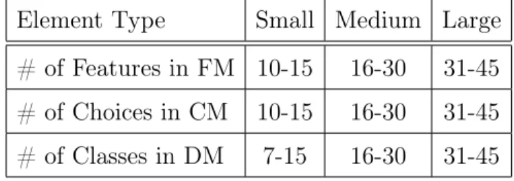
Element Type Small Medium Large

# of Features in FM 10-15 16-30 31-45

# of Choices in CM 10-15 16-30 31-45

# of Classes in DM 7-15 16-30 31-45

Table 6.1. Number of elements in each category

# Property

R4 @ Association A in DM: (A.from = none OR A.to=none)

R5 @ Class C in DM: ∀ Association A in DM (C not in A.from) AND (C not in A.to)

R6 @ Association A in DM: (A.from =A.to)

Table 6.2. Properties Checked for scalability analysis

models. For this, we used the class diagrams of the metamodels from the AtlanMod

Metamodel Zoo [18]1

According to their size, we categorize feature models, choice models and domain models in three categories: small, medium and large. To generate the complete SPLDCs, we combine feature models, choice models and domain models from all three categories to generate 270

different SPLDCs, belonging to 27 different categories. Table 6.1 shows the number of

elements in each category.

We generated random feature mappings and decision mappings for these SPLDCs. We then transformed all Tyson models to Alloy specifications.

We checked the three consistency properties shown in Table 6.2 for each model and recorded the run times to check the scalability of the approach. To study the effect of Alloy’s scope in the analysis, we tried scopes of 20, 40, and 60. The results of property analysis were same regardless of scope, however the analysis became much slower. Below, we report results for scope 40. The machine we used to run these experiments is a LENOVO ThinkPad laptop, with 8GB RAM and Intel(R) Core(TM) i5-7200U CPU @ 2.50GHz, 2701 Mhz, 2 Core(s), 4 Logical Processor(s).

1. http://web.imt-atlantique.fr/x-info/atlanmod/index.php?title=Zoos

(47)

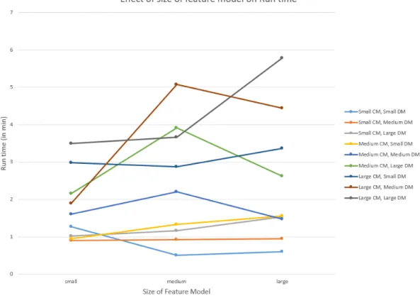
Figure 6.1. Effect of size of feature model on run time for different sizes of choice model and domain model

6.2. Results

To assess the scalability of the approach, we study how the run time for each check varies with the size of different elements of SPLDC. Figure 6.1, Figure 6.2, and Figure 6.3 shows the effects on the run time of the size of feature model, choice model and domain model respectively. The maximum time for a check was approximately 6 minutes for the category with large feature models, large choice models, and large domain models. Figure 6.1 shows a mixed trend in run time with respect to the size of feature models. On one hand, for some categories run time increases with increasing size of feature models. On the other hand, for some categories run time decreases despite an increase in the size of feature model.

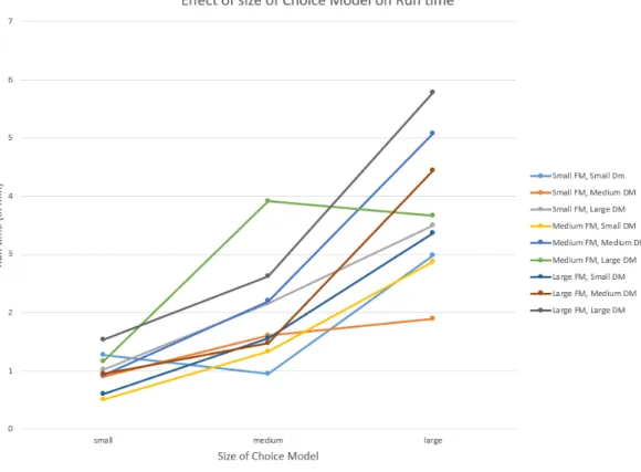
However, figure 6.2 shows that in most of the cases, run time increases with increase in size of choice models.

(48)

Figure 6.2. Effect of size of choice model on run time for different sizes of feature model and domain model

Figure 6.3 shows that for the majority of the categories run time increases with increase in domain model size. However, there are some categories where run time decreases despite increase in domain model size.

6.3. Discussion

According to the results for the scalability study, we can see that in general for large SPLDCs, the run time for each check can take a few minutes. Figure 6.2 shows that size of choice model clearly impacts the run time. So, we conclude that for SPLDCs with more uncertainty, run time is larger. Figure 6.4 shows that Alloy scope has significant impact on the run time. Higher value of scope means higher confidence over the results as Alloy then considers larger expressions while analyzing a property, but that also leads to an increase in the run time. So, there is a trade-off between run time and confidence over the results. However, for the examples that we studied, we get the same results even increasing the scope. Hence, by considering the small scope hypothesis explained in Chapter 2, we set scope to

(49)

Figure 6.3. Effect of size of Domain model on run time for different sizes of choice model and Feature model

be 40 for our experiments. Overall, we note that with increasing the sizes of the different SPLDC components indicates some reasonable increases in run time. In other words, we do not see evidence that increasing the size of any of the components of an SPLDC can have a dramatic effect in the overall scalability of the approach. Even though the property checks took some minutes to complete, the overall cost did not outweigh the benefit of being able to reason in the presence of both variability and uncertainty in SPLDCs.

6.4. Threats to validity

Our evaluation is faced with various threats to the validity, discussed briefly below. One threat to validity comes from our choice of experimental subjects. To mitigate the lack of real examples, we randomly generated SPLDCs. For this, we used real, publicly available models from SPLOT and the AtlanMod Metamodel Zoo, and only randomly generated the mappings. This allowed us to generate SPLDCs of various sizes, allowing us to explore the effect of the change in size. To mitigate the randomness, we used real

(50)

Figure 6.4. Effect of scope on run time

components (domain, feature and choice models) to generate SPLDCs. We are therefore confident that the resulting SPLDCs are realistic.

A second threat to validity comes from our choice or properties. To mitigate this, we chose examples of properties that were inspired from published literature and represent typical structural properties of models found in MDE practice.

The choice of Alloy scope may also affect the results. To mitigate this effect, we experi-mented with various scopes, validating that the choice of scope did not change the property check results. Regardless, we report observations for a high enough scope such that the slowdown effects would be observable.

In the future we intend to experiment with even larger examples, as well as with other reasoning engines such as Clafer [37], and Alloy* [26] and alternative automated reasoning formalisms, such as QBF solving [20] and Answer Set Programming [22], with the aim to improve the efficiency of the implementation.