HAL Id: hal-00920567
https://hal.archives-ouvertes.fr/hal-00920567
Submitted on 18 Dec 2013
HAL is a multi-disciplinary open access
archive for the deposit and dissemination of
sci-entific research documents, whether they are
pub-lished or not. The documents may come from
teaching and research institutions in France or
abroad, or from public or private research centers.
L’archive ouverte pluridisciplinaire HAL, est
destinée au dépôt et à la diffusion de documents
scientifiques de niveau recherche, publiés ou non,
émanant des établissements d’enseignement et de
recherche français ou étrangers, des laboratoires
publics ou privés.
Using Polynomial Wigner-Ville Distribution for Velocity
Estimation in Remote Toll Applications
Stéphane Meric, Rébecca Pancot
To cite this version:
Stéphane Meric, Rébecca Pancot. Using Polynomial Wigner-Ville Distribution for Velocity Estimation
in Remote Toll Applications. IEEE Geoscience and Remote Sensing Letters, IEEE - Institute of
Electrical and Electronics Engineers, 2014, 11 (2), pp.409 - 413. �hal-00920567�
Ville distribution (PWVD) for accurate velocity estimation as used in remote road traffic management applications. In such applica-tions based on inverse synthetic aperture radar, velocity estimation is central to obtain a suitable level of performance of the signal processing. Moreover, the precision of this velocity estimation is crucial in order to achieve the best detection and estimation of the gauge of the vehicles through the use of radar images. Hence, the PWVD is applied as an instantaneous frequency estimator used in this traffic surveillance application.
Index Terms—Polynomial Wigner–Ville distribution (PWVD),
radar applications, radar imaging, remote toll applications, signal processing, time–frequency processing, velocity measurement.
I. INTRODUCTION
R
ADAR imaging can be considered as a process of map-ping the electromagnetic reflectivity of a target from multiple-aspect data. Angular diversity can be acquired through the relative movement between the target and the sensor. Thus, inverse synthetic aperture radar (ISAR) processing is used to separate scattering points of a moving target [1]. These scattering points describe a large part of the electromagnetic re-flectivity of the target and can modelize the shape of this target [2]. The aim of this letter is to present an opportunity to estimate the velocity of a vehicle with a view to achieving its radar image using ISAR processing. In ISAR, several methods are necessary to compensate the target motion in order to obtain focused images. These methods usually are processed in two steps and are known as range-bin alignment and phase adjustment [3]. In our case, as is described in Section II, the radar imagery method we develop only needs the value of the target translational velocity. Hence, in order to obtain focused ISAR images, it is essential to obtain as precisely as possible this value of velocity. In a microwave context [4] or sonar context [5], the obtaining achieving velocity commonly makes use of the Doppler effect. It is well known that the velocity of the target is proportional to the maximum Doppler spread fD of the reflected signalby the target throughfD= (2πvfc)/c, where fcis the carrier
frequency, andc is the speed of propagation. Thus, estimating v andfDare equivalent. However, regardless of the applications,
Manuscript received September 19, 2012; revised April 2, 2013; accepted May 6, 2013.
S. Méric is with the Institute of Electronics and Telecommunication of Rennes (IETR), 35042 Rennes, France (e-mail: stephane.meric@ insa-rennes.fr).
R. Pancot is with the French National Defence Agency, DGA-Essais en vol, Cazaux, France.
Color versions of one or more of the figures in this paper are available online at http://ieeexplore.ieee.org.
Digital Object Identifier 10.1109/LGRS.2013.2263576
Doppler estimation methods are also compared on the basis of their ability to provide precise Doppler estimation. To achieve this accuracy, a solution consists of designing large bandwidth signals that provide good Doppler measurement capability but requires a long duration for processing [7]. Moreover, if the antenna has a large beam and is located very close to the passing target, for instance, the Doppler frequency quickly varies, and the presence of nonlinear phase function in the reflected signal makes it difficult to extract the target motion [8]. Consequently, standard Fourier transform is inadequate to extract the Doppler information from such reflected signals. Thus, most velocity-determining methods are based on joint time–frequency analysis, which are specifically dedicated to process nonstationary signals [9], and the effectiveness of the time–frequency methods has been widely demonstrated for sig-nal processing in applications such as radar [10], optoelectronic [11], acoustic [12], or biology [13].
This letter focuses on an efficient method of velocity esti-mation based on time–frequency analysis and destined for a remote toll context. The specific geometry of our remote toll system and the requirements of our imaging application lead us to choose a polynomial Wigner–Ville distribution (PWVD) to extract target velocity from the received signal.
II. CONTEXT
The backdrop of our application is the traffic congestion that occurs when many vehicles approach the toll area. An efficient solution to overcome this problem is the use of remote toll payment systems, so that the traffic freely moves. Thus, the operational area of the application presented in this letter is a drive-by toll system. In order to prevent fraud, an imaging processing function based on ISAR is integrated without chang-ing anythchang-ing in the existchang-ing system. Thus, the system makes it possible to verify the presence of a transponder badge inside the vehicle while matching of the size of the vehicle and the size indicated by the badge.
In our case, the system transmits a continuous wave when a vehicle passes under the toll beacon in order to get information (type of vehicle) from an identification badge positioned inside the vehicle (see Fig. 1). The transaction payment is carried out due to this identification badge. Our objective is to add an imaging function to classify the vehicles for traffic monitoring and to verify that the size of the vehicle matches the information on the identification card. Thus, this imaging function makes it possible to classify the vehicles (by height) by establishing the radar image of vehicles.
410 IEEE GEOSCIENCE AND REMOTE SENSING LETTERS, VOL. 11, NO. 2, FEBRUARY 2014
Fig. 1. Geometry of the problem.
The radar imaging methods are used to separate scattering points at a certain distance from the radar. Generally, a scatter-ing pointi is characterized by its spatial location (xi, zi) and by
its reflectivity σi. Thus, a radar scenef (x, z) can be described
by an area reflectivity functionf (x, z) =!
iσiδ(x − xi, z −
zi). The radar image formation aims at evaluating this area
reflectivity function in the spatial domain and is based on a 2-D theory supported by range and cross-range imaging techniques. ISAR processing consists of applying 2-D matched filtering on the received signal that is scattered by pointsi. Thus, one retrieves the target function described byf (x, z). A vehicle is considered as a set of such scattering pointsi [2]. At this time of the study, to simplify the problem, we assume that the scattering pointsi are only located in the (Oxz) plane. Moreover, during the illumination time, the vehicle is assumed to move under the antenna on a linear path (along thex-axis) with constant veloc-ityV . The response from one scattering point i initially located at(xi0, zi0) is the transmitted signal delayed by the round trip
of the wave and weighted by propagation attenuation (defined byA′
), antenna gain (described by the functiong(x, z)) and the reflectivity coefficient (given by σi). Thus, the signal received
by the antenna is the sum of the contributions ofN scattering pointsi, i.e., sr(t) = A′ N " i=1 σi.g2(xi0−V t, zi0).e # 2πfc # t−2Di(t)c $ +φ0$ (1) where Di(t) is the evolutive distance (see Fig. 1), φ0 is an
unknown phase, andfcis the carrier frequency (in our
applica-tion,fc= 5.8 GHz) between the radar and the scattering point
i during the illumination time T , i.e., Di(t) =
% D2
0i+ (V t)2−2 D0iV t cos(α0i) (2)
where D0i and α0i describe the initial location (att = 0) of
the ith point according to Fig. 1. Our imaging procedure is based on the correlation between signal sr(t) and a replica.
This replica is defined in the scene that corresponds to the area where the target can be seen by the radar. For example, for a point located atz = 0.5 m, we can see in Fig. 2 the point-spread function (PSF) provided by electromagnetic simulating and by taking into account the radiation pattern of the antenna (βh= 35.22◦) and the elevation angle (αe= 30◦). Moreover,
this PSF provides the theoretical azimuth resolution δx =
Fig. 2. PSF of the imaging method.
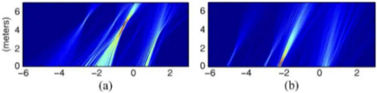
Fig. 3. Vehicle under test and the corresponding radar image. (a) Vehicle under test. (b) Radar image (scattering points) of the vehicle under test.
Fig. 4. Consequences on radar image of 10% relative error of velocity estimation. (a) Underestimated velocity. (b) Overestimated velocity.
λc/(4 sin(βh/2) cos(αe)) and height resolution δz ≈ 10 δx
de-scribed in [14]. Our processing is tested with measured signals obtained due to a remote toll payment beacon provided by CS-SI (Compagnie des Signaux-Systèmes d’Information, a French company, which supplies toll road operations). The experiments are conducted in a controlled scene and the measurement conditions are the following: H = 3.43 m, βh= 35.22◦, and
αe= 30◦. Moreover, the time duration of the reflected signal
recording is around 0.5 s. It is worth noting that the level of the sidelobes of the antenna pattern is −29 dB below the mainlobe level. Thus, we can consider that the effect of the returned signal through the sidelobes is insignificant in this case. Moreover, the Doppler effect induced by the vehicle passing through the origin is also almost negligible. Finally, we indicate that the coherent processing interval fit with the inverse of the maximum Doppler spreading generated by the vehicle. As an example, we present a radar image [see Fig. 3(b)] that we obtain considering the vehicle under test [see Fig. 3(a)]. Thus, we can say this radar image shows us the location of the main scattering points that we can anticipate on this kind of vehicle (particularly, the wedge boundary at the end of the top roof, i.e., point 1; the wedge boundaries between the two top roofs of the vehicle, i.e., points 2 and 3; and the wedge boundaries of the bonnet, i.e., points 4 and 5). At this step, it is important to note that this radar image is computed due to the velocity of the vehicle measured by a police lidar system during the experimental measurement. Thus, the accuracy of
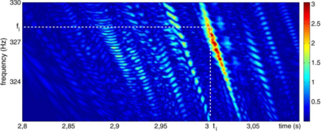
Fig. 5. Polynomial Wigner–Ville (sixth-order) mapping for the measured signal.
the velocity estimation (less than 3% according to the operating lidar system) is sufficient to provide the image quality one can see in Fig. 3(b). However, during operating mode, this velocity information of the passing vehicle is not provided by police radar. Thus, we have to extract from the reflected signal the translational velocity with sufficient accuracy.
In order to evaluate the influence of the velocity accuracy measure, we compute the radar image by changing the value of the velocity regarding the real value, which is measured by the lidar and provides the radar image shown in Fig. 3(b). The main effect of bad velocity estimation is that the scattering points are unfocused and are not properly located (see Fig. 4). Thus, for this first study, we consider that the maximum relative error of a scattering point position is about 10%. Based on this assumption, the relative error of the estimation of velocity V must be less than 5%. Consequently, depending on the surrounding infrastructure we use, the measurement conditions make it impossible to estimate the transverse and the axial components of the velocityV by using conventional Doppler techniques, whereas the achievement of signal processing for radar images requires a reasonably good estimation of this velocity.
III. VELOCITYESTIMATIONSCHEME
A. Instantaneous Doppler Frequency and Velocity
The next step is to determine the velocity of the vehicle. Our scheme is mainly supported by one assumption: there is at least one scattering pointi, which induces a maximum value of the reflected signal amplitude when this pointi passes the line of sight of the antenna (see Fig. 1) at time t0. This assumption
is essentially based on our own investigations consisting of electromagnetic simulations. Vehicles are modelized by sheets of metal or specific dielectric properties such as the wind-screen that describes the vehicles’ structures. The physical optic method is applied to generate the whole electromagnetic field reflected from a vehicle under test. Consequently, these simu-lations make it possible to extract scattering centers of vehicles as described in [2]. Hence, there is at least one scattering center that induces one maximum magnitude of the reflected signal. This maximum is obtained when the scattering center passes
through the line of sight of the antenna that corresponds to a specular situation. Thus, velocityV of the vehicle is given by
V = fDi(t0)λc
2 sin αe (3)
where λcis the wavelength of the carrier frequency, andfDi(t0)
is the instantaneous Doppler frequency attached to the pointi at timet0. Moreover, in order to locate as precisely as possible the
position of the maximum amplitude, we carry out a smoothing operation applied on the baseband signal srb(t) from sr(t)
to obtain the smooth signal ˆsrb(t). This smoothing operation
involves a Hamming weighted functionH(.) of length M . We can expresssˆrb(t) with
ˆ srb(t) = 1 M M/2 " τ =−M/2 |srb(t + τ )| .H(τ ). (4)
We obtaint0asˆsrb(t0) ≥ ˆsrb(t) regardless of the value of t.
B. Frequency Modulated Law
The frequency modulated law of the reflected signal from a passing vehicle is based on the assumption that this vehicle is considered as a set of scattering points i (see Fig. 1). Moreover, at this step of the process, we consider that this vehicle moves at a constant speed throughout the observation periodT . Thus, the received signal by the antenna is the sum of the contributions of N scattering points i. This signal is described by relation (1) and can be rewritten more simply with the following relationshipsr(t) = A′exp(φr(t)), where φr(t)
is the phase of the received signal. Thus, the instantaneous frequency finst(t) of signal sr(t) defined with (1) is derived
from phase φr(t). As number N of scattering points increases,
the expression of finst(t) becomes complex and unsuited to
velocity estimation based on the conventional Doppler method. However, one particular method of instantaneous frequency estimation is based on the time–frequency representation of the signal. This time–frequency representation is a 2-D function, which attempts to show the distribution of the signal energy in a joint time–frequency plane (see Fig. 5). Thus, for a given value of timeti, the maximum modulus of the time–frequency
412 IEEE GEOSCIENCE AND REMOTE SENSING LETTERS, VOL. 11, NO. 2, FEBRUARY 2014
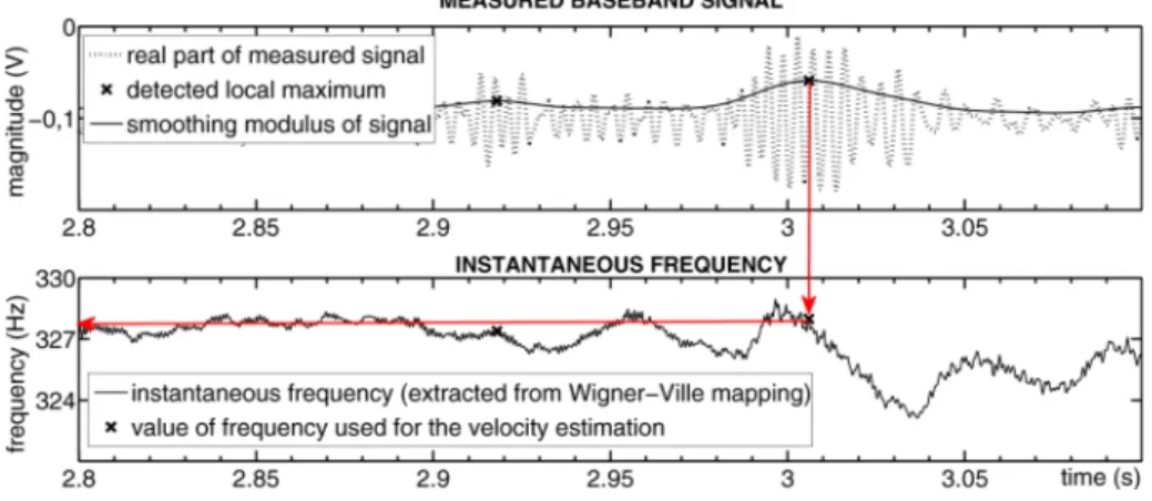
Fig. 6. (Up) Measured baseband signal srb(t) and |ˆsrb(t)| and (down) the instantaneous frequency extracted from the PWVD mapping.
C. PWVD
The simplest way to extract the instantaneous frequency from a signal is the short-time Fourier transform (STFT) by dividing the signal into small time window segments and applying a Fourier transform to each segment. For each window, the spec-tral centroid method is used to obtain the first moment of the power spectrum and the velocity map is provided by computing all these first moments. Nevertheless, the performance values of the STFT are related to the choice of the window, which is a drawback compared with the WVD [15]. The WVD is known to provide maximum localization of the signal energy, which can be related to the true instantaneous frequency. The WVD is particularly appropriate to linear frequency modulated signals [16] that correspond to a second-order polynomial phase law. In our case study, (1) practically exhibits a higher order instan-taneous frequency law. Thus, theqth-order PWVD (PWVDq)
provides an optimal time–frequency representation of a signal having a phase law of polynomial order lower thanq [17]. The PWVDq is defined using the Fourier transform of aqth-order
kernel functionKq(t, τ ), then
PWVDq(t, f ) = & τ Kq(t, τ )e−2πf τdτ Kq(t, τ ) = q/2 ' k=0 z(t + ckτ)bkz∗(t + c−kτ)−bk. (5)
Expression z(t) is the analytic signal associated with sr(t)
andz∗(t) denotes the conjugate complex of z(t). The
imple-mentation ofKq requires some properties ofbk andck [18].
For the specific case of our work, we propose to compare the performance of the fourth-order and sixth-order kernels defined in [19] that correspond to the complexity of the different shapes of vehicles under measurement and the operating conditions. We have to note that a signal-to-noise ratio (SNR) larger than 3 dB makes PWVDqpossible to be efficient [17]. The peak of
the PWVDq given by (5) provides the value offDi(t0) at this
timet0, and we can compute velocityV using (3).
IV. MEASUREMENTRESULTS
First, as an example, we illustrate the use of PWVD with a reflected baseband signal from a small lorry (height of 2.5 m)
TABLE I
RELATIVEERROR(MEANmANDSTANDARDDEVIATIONσ) (%) BETWEEN THEVELOCITYCALCULATEDWITHOUR
PROCESSING AND THEVELOCITYMEASURED
WITH THEPOLICELIDAR
passing under the remote toll beacon with αe= 30◦. During
the acquisition time, the vehicle is assumed to move along the (Ox) axis and with a constant velocity V . We expose in Fig. 5 the modulus of PWVD6 applied on the reflected signal. Thus,
we obtain the instantaneous frequencyfiby localizing the
max-imum value of the modulus of PWVD6for each value of time
ti. In Fig. 6, we correspond two local maximums of|ˆsrb(t)| to
their instantaneous frequency, respectively. The instantaneous frequency curve is extracted from the PWVD mapping. In this example, the velocity is estimated at43.2 km · h−1
compared with the velocity of 44 km · h−1
obtained with a police lidar system during the measurement.
Second, we acquire reflected signal data corresponding to a car and a lorry moving at various velocities. Moreover, we consider two different elevation angles (30◦
and 45◦
). We compute through our processing of these data sets to obtain the values of velocity Vp. These values are also compared
with thoseVmobtained with the police lidar system. Thus, we
calculate the relative error (%) between Vp and Vm. Table I
gives the results as a couple (m, σ), where m is the mean value, and σ is the standard deviation of the relative errors. The values (m, σ) are obtained by processing 30 different velocities (Vm∈[10; 50] km · h−1) for each vehicle and each value of αe.
The considered trials are chosen to meet speed limits allowed when vehicles approach the toll area. Moreover, we consider the influence of PWVD4 and PWVD6 on the results. We
compare these with the results we obtain using the WVD, which is dedicated to linear frequency modulated signals and also the STFT.
type. Moreover, it seems more difficult to have the expected accuracy forVp(relative error less than 5%) if we consider the
results obtained with the car. These observations mean that the geometric conditions influence the accuracy of the computing velocity Vp and the shape of vehicles under test. Actually,
considering the energy distribution on the time–frequency map-ping, the more concentrated the energy is in a very small area, the more accurate the instantaneous frequency value will be. In other words, when the scattering points pass through the line of sight of the antenna, the sharper the response of these points is, the more precise the output of the PWVD will be. Moreover, by considering relation (3), an error∆fDi(t0) induces a greater
error ∆V for low elevation angles αe than for high ones.
Another explanation of these results concerns the slope of the instantaneous frequency curve versus time, which is lower for high elevation angles than for low ones. Consequently, a bad assessment oft0, i.e.,fDi(t0), induces a final accurate value of
V that is less satisfactory for low elevation angles than for high ones. Nevertheless, as indicated in Section III, a SNR level of at least 3 dB is required to accurately perform the instantaneous frequency by using the PWVD. Thus, setting a high elevation angle αe tends toward a decrease in the SNR of the received
signal that also depends on the vehicle shapes.
It is worth noting that there is another method based on the image quality measurement to obtain an ISAR image [20]. This method called contrast optimization makes use of a cost function to measure the degree of focus of the ISAR image. This cost function can be chosen as an entropy function or contrast function. Nevertheless, the traffic surveillance application we are developing requires real-time information and low-complexity calculation. Consequently, the contrast optimization method fails to meet these requirements when compared with Wigner distributions, which provide results by using a fast Fourier transform network half the size of the one needed to perform a STFT [21].
VI. CONCLUSION ANDFURTHERDEVELOPMENT In this letter, we have proposed a procedure to estimate the velocity of a vehicle in the case of a specific application. This velocity is used to provide a radar image of this vehicle that will be used in road traffic management. Considering the specific geometric conditions, we show that the PWVD provides a velocity measurement, which is sufficiently accurate for the signal processing in order to obtain radar images. Nevertheless, our study shows that the accuracy of the calculated velocity also depends on the geometric conditions and the vehicle type. Thus, it would be interesting to extend these first conclusions
IEEE Trans. Aerosp. Electron. Syst., vol. AES-16, no. 1, pp. 2–14, Jan. 1980.
[2] K. Schuler, D. Becker, and W. Wiesbeck, “Extraction of virtual scattering centers of vehicles by ray-tracing simulations,” IEEE Trans. Antennas Propag., vol. 56, no. 11, pp. 3543–3551, Nov. 2008.
[3] C. Ozdemir, Inverse Synthetic Aperture Radar Imaging With Matlab Algorithms. Hoboken, NJ, USA: Wiley, 2012.
[4] P. Fisher, “Improving on police radar,” IEEE Spectr., vol. 29, no. 7, pp. 38– 43, Jul. 1992.
[5] Y. Doisy, L. Deruaz, S. Beerens, and R. Been, “Target Doppler estima-tion using wideband frequency modulated signals,” IEEE Trans. Signal Process., vol. 48, no. 5, pp. 1213–1224, May 2000.
[6] C. Tepedelenlioglu and G. Giannakis, “On velocity estimation and corre-lation properties of narrow-band mobile communication channels,” IEEE Trans. Veh. Technol., vol. 50, no. 4, pp. 1039–1052, Jul. 2001.
[7] G. Jourdain and J. Henrioux, “Use of large bandwidth-duration bi-nary phase shift keying signals in target delay Doppler measurements,” J. Acoust. Soc. Amer., vol. 90, no. 1, pp. 299–309, Jul. 1991.
[8] Q. Wang, M. Pepin, R. J. Beach, R. Dunkel, T. Atwood, B. Santhanam, W. Gerstle, A. W. Doerry, and M. M. Hayat, “SAR-based vibration es-timation using the discrete fractional Fourier transform,” IEEE Trans. Geosci. Remote Sens., vol. 50, no. 10, pp. 4145–4156, Oct. 2012. [9] P. Kersten, R. W. Jansen, K. Luc, and T. L. Ainsworth, “Motion analysis in
SAR images of unfocused objects using time-frequency methods,” IEEE Geosci. Remote Sens. Lett., vol. 4, no. 4, pp. 527–531, Oct. 2007. [10] T. Thayaparan, G. Lampropoulos, S. K. Wong, and E. Riseborough,
“Ap-plication of adaptive joint time-frequency algorithm for focusing distorted ISAR images from simulated and measured radar data,” Proc. Inst. Elect. Eng.—Radar, Sonar Navig., vol. 150, no. 4, pp. 213–220, Aug. 2003. [11] Z. Xu, L. Carrion, and R. Maciejko, “An assessment of the Wigner
distri-bution method in Doppler OCT,” Opt. Exp., vol. 15, no. 22, pp. 14 738– 14 749, Oct. 2007.
[12] D. C. Reid, A. M. Zoubir, and B. Boashash, “Aircraft flight parameter estimation based on passive acoustic techniques using the polynomial Wigner-Ville distribution,” J. Acoust. Soc. Amer., vol. 102, no. 1, pp. 207– 223, Jul. 1997.
[13] A. Monti, C. Medigue, and L. Mangin, “Instantaneous parameter esti-mation in cardiovascular time series by harmonic and time-frequency analysis,” IEEE Trans. Biomed. Eng., vol. 49, no. 12, pp. 1547–1556, Dec. 2002.
[14] R. Giret, S. Méric, and G. Chassay, “2D Radar image of moving vehicles from 1D-signal using SAR processing,” in Proc. Eur. Conf. Synthetic Aperture Radar, May 2002, pp. 633–636.
[15] L. Cohen, Time-Frequency Analysis. Englewood Cliffs, NJ, USA: Prentice-Hall, 1995, ser. Prentice Hall Signal Processing Series. [16] B. Boashash, P. O’Shea, and M. J. Arnold, “Algorithms for instantaneous
frequency estimation: A comparative study,” in SPIE Proc.—Advanced Signal Processing Algorithms, Architectures, Implementations, Nov. 1990, vol. 1348, pp. 126–148.
[17] B. Barkat and B. Boashash, “Instantaneous frequency estimation of poly-nomial FM signals using the peak of the PWVD: Statistical performance in the presence of additive Gaussian noise,” IEEE Trans. Signal Process., vol. 47, no. 9, pp. 2480–2490, Sep. 1999.
[18] B. Boashash and P. O’Shea, “Polynomial Wigner-Ville distributions and their relationship to time-varying higher order spectra,” IEEE Trans. Sig-nal Process., vol. 42, no. 1, pp. 216–220, Jan. 1994.
[19] B. Barkat and B. Boashash, “Design of higher order polynomial Wigner-Ville distributions,” IEEE Trans. Signal Process., vol. 47, no. 9, pp. 2608– 2611, Sep. 1999.
[20] L. Xi, L. Guosui, and J. Ni, “Autofocusing of ISAR images based on entropy minimization,” IEEE Trans. Aerosp. Electron. Syst., vol. 35, no. 4, pp. 1240–1252, Oct. 1999.
[21] N. Bergmann, “New formulation of discrete Wigner-Ville distribution,” Electron. Lett., vol. 27, no. 2, pp. 111–112, Jan. 1991.